When labeling L2 users as nativelike or not, consider classification errors
Jan Vanhove University of Fribourg
Author note
I thank Raphael Berthele, David Birdsong, David Singleton, and the anonymous SLR reviewers for their comments.
Correspondence concerning this article should be addressed to Jan Vanhove, University of Fribourg, Department of Multilingualism, Rue de Rome 1, CH-1700 Fribourg, Switzerland. E-mail: [email protected].
Accepted version (without type-setting and copy-editing). For the published version, see:
Vanhove, Jan. 2019. When labeling L2 users as nativelike or not, consider classification errors. Second Language Research.
doi:10.1177/0267658319827055 1 2 3 4 5 6 7 8 9
Abstract
Researchers commonly estimate the prevalence of nativelikeness among second-language learners by assessing how many of them perform similarly to a sample of native speakers on one or several linguistic tasks. Even when the native and L2 samples are comparable in terms of age, socio-economic status, educational background and the like, these nativelikeness estimates are difficult to interpret theoretically. This is so because it is not known how often other native speakers would be labeled as non-nativelike if judged by the same standards: if some other native speakers were to be labeled as non-nativelike, then it is possible that some second-language learners that were categorized as non-nativelike are actually nativelike. Two methods for estimating the classification error rate in nativelikeness categorizations—one conceptually straightforward but practically arduous, and one involving the reanalysis of the original studies’ data—are proposed. These approaches underscore that, even if one conceives of nativelikeness as a binary category (nativelike vs. non-nativelike), the data collected in any given study may not allow for such neat categorizations.
Keywords: age factor in second language acquisition, classification, critical period hypothesis, nativelikeness
Word count: 6682, everything included. 10 11 12 13 14 15 16 17 18 19 20 21 22 23 24 25 26
When labeling L2 users as nativelike or not, consider classification errors
Who, if anyone, can achieve a nativelike command of their second language (L2)? This question undergirds a considerable body of research, particularly with respect to the ‘age factor’ in second language acquisition (Birdsong, 2005; Long, 2005). Estimates of the prevalence of nativelikeness in L2 speakers are typically obtained by assessing how many of a sample of L2 speakers perform similarly to a sample of L1 controls on one or several linguistic tasks. Here I will first argue that published estimates of the pervasiveness of nativelikeness among L2 speakers are difficult to interpret. This is so because they are not accompanied by an estimate of the rate at which other native speakers than the native controls recruited in the study would be flagged as non-nativelike by the same standards. This rate can be substantial, even when these other native speakers are drawn from the same population as the native controls in terms of age, education, socio-economic status, region, etc. Then I will suggest two ways in which this error rate can be estimated in a specific study. The first way is to recruit an additional set of L1 controls whose nativelikeness is judged by the same standards used to categorize the L2 speakers. The second way is to reanalyze the study’s data with statistical classification models that can output such error rate estimates.
This article concerns a strictly statistical point pertinent to nativelikeness studies, but two related criticisms often leveled at nativelikeness studies ought to be briefly mentioned first. The first of these is that the concept of nativelikeness and comparisons of L1 vs. L2 speakers are not necessary or even not useful in research on the age factor and more generally (see, among others, Birdsong & Gertken, 2013; Birdsong & Vanhove, 2016; Cook, 1992; Davies, 2003; Grosjean, 27 28 29 30 31 32 33 34 35 36 37 38 39 40 41 42 43 44 45 46 47
1989; Ortega, 2013). The second is that the samples of L1 and L2 speakers are not always
comparable in terms of age, socio-economic status, educational background, etc. Inasmuch as the amount and kind of linguistic knowledge varies along these dimensions (e.g., Dąbrowska, 2012), the yardstick against which L2 speakers are judged will differ depending on the make-up of the L1 sample (also see Andringa, 2014). Rather than discuss these two criticisms, I will argue that if researchers do want to estimate the prevalence of nativelikeness in a population of L2 speakers by comparing a sample of them to a sample of L1 speakers drawn from an appropriate
population, then they should also estimate how often different L1 speakers drawn from the same population will falsely be identified as non-nativelike based on the same criteria by which the L2 speakers were judged. My suggestions for estimating error rates in nativelikeness studies cannot resolve the usefulness and comparability criticisms and are offered in the understanding that these criticisms have been adequately addressed. That said, my suggestions do naturally highlight that, even if one wants to uphold the nativelike vs. non-nativelike distinction theoretically, the data may not allow for such neat categorizations in any given study.
Nativelikeness criteria and their miss rates
Range- and standard deviation-based nativelikeness criteria
Perhaps the most ambitious project on nativelikeness in L2 speakers is the
“non-perceivable non-nativeness” approach by Hyltenstam and Abrahamsson (2003). They suggested that while some proportion of L2 speakers may be perceived by native speakers as native speakers, even these L2 speakers would still differ from native speakers in linguistically subtle ways. In a follow-up to this suggestion, Abrahamsson and Hyltenstam (2009) subjected 41 highly 48 49 50 51 52 53 54 55 56 57 58 59 60 61 62 63 64 65 66 67 68
proficient L2 speakers of Swedish, who had previously been identified as nativelike by native speakers, to 10 linguistic tasks. Fifteen L1 speakers of Swedish also completed the same tasks. On the basis of the L1 speakers’ scores, intervals representing nativelike performance were constructed. Specifically, a participant’s performance on a task was considered nativelike if it fell within the range (i.e., between the sample minimum and the sample maximum) of the L1
speakers’ performance on the task. Of the 41 highly proficient L2 speakers, only “two, possibly three” (p. 283) passed the nativelikeness criterion on all 10 tasks. Some other examples where nativelikeness is operationalized in terms of the statistical range of the performance of a sample of native controls are Abrahamsson (2012), Birdsong and Molis (2001), Bylund, Abrahamsson & Hyltenstam (2012), Coppieters (1987), Flege, Munro, and MacKay (1995), Flege,
Yeni-Komshian, and Liu (1999), Hopp and Schmid (2013), Johnson and Newport (1989), Patkowski (1980), and Van Boxtel, Bongaerts, and Coppen (2005).
Some researchers, rather than basing themselves on the statistical ranges of task scores in native speaker controls, constructed the nativelikeness interval in terms of a number of standard deviations (SDs) around the native controls’ mean task scores. (Confusingly, even intervals based on standard deviations rather than ranges are called ‘native ranges.’) For instance, Andringa (2014) defined the nativelikeness criterion as the native controls’ mean plus two standard
deviations for speed tasks or the mean minus two standard deviations for accuracy tasks. Similar intervals have been applied by, among others, Birdsong (2007), Bongaerts (1999), Díaz, Mitterer, Broersma, and Sebastián-Gallés (2012), Flege et al. (1995), Huang (2014), and Laufer and Baladzhaeva (2015). 69 70 71 72 73 74 75 76 77 78 79 80 81 82 83 84 85 86 87 88 89
Miss rates
It is readily recognized that L2 speakers whose performance on one or several tasks is judged to be nativelike according to range- or standard deviation-based criteria may be non-nativelike in other respects: non-nativelike performance on a battery of tasks does not imply across-the-board nativelikeness (Abrahamsson & Hyltenstam, 2009; Long, 2005). But even some native speakers may not pass the criteria set by the control sample either—not even if they were drawn from the population as the native controls in terms of region, education, knowledge of other languages, socio-economic status etc., and were focused and not having an off-day. The possibility that some native speakers may not pass a set of nativelikeness criteria implies that some L2 speakers who were identified as non-nativelike may yet be nativelike: the criteria may have been too strict.
My point is not so much that if a set of nativelikeness criteria is based on a sample of young, highly educated speakers of the L1 standard language who grew up and live in a monolingual environment, some elderly, less educated, dialectal, bilingual or attriting L1 speakers may not pass this mark—however true and relevant this is (e.g., Andringa, 2014). Rather, it is that even some young, highly educated speakers of the L1 standard language who grew up and live in a monolingual environment may not meet all criteria either. If researchers ignore this possibility, they essentially assume that nativelikeness criteria have some false alarm rate (L2 speakers could have wrongly been categorized as nativelike, e.g., because they had not been tested in sufficient detail) but no miss rate (no native speakers will wrongly be categorized as non-nativelike). 90 91 92 93 94 95 96 97 98 99 100 101 102 103 104 105 106 107 108 109 110
Estimating a set of nativelikeness criteria’s miss rate is essential for a theoretically sensible interpretation of the nativelikeness estimates it yields. Suppose that 100 advanced L2 speakers and 32 native controls (both sampled from appropriate populations) participate in a particularly challenging task battery. Judging by the standards set by the 32 controls, not a single L2 learner is identified as nativelike on this battery. Now suppose that 100 additional native speakers, sampled from the same population as the original controls, are recruited and judged by the same standards. In principle, it is possible that some of them would fail to meet the set of nativelikeness criteria that was constructed on the basis of the 32 original controls. This
possibility exists if some of the nativelikeness intervals that were constructed on the basis of the native controls are narrower than the respective ranges in the native-speaker population. This possibility, in turn, would force us to consider the possibility that some L2 speakers might have been wrongly categorized as non-nativelike, too: if 15% of the new sample of native speakers fail to meet the nativelikeness criteria to which the L2 speakers were held, this would imply that some 15% of the L2 speakers may (not ‘will’) have been wrongly identified as non-nativelike, too.
Miss rates for a single task score
The miss rates in nativelikeness studies depend on a number of factors, which I
investigated by means of simulations. Simulations have the advantage that they allow us, for the time being, to disregard empirical challenges, such as how to define the appropriate population of native speakers and then randomly sample from it. The simulations below, then, concern a best-case scenario. The simulation code and the results are available from https://osf.io/pxefv/. 111 112 113 114 115 116 117 118 119 120 121 122 123 124 125 126 127 128 129 130 131
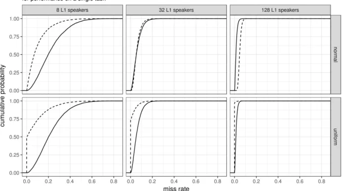
Let us first focus on miss rates for a single task, and more specifically on three factors: (a) the size of the native control sample, (b) how the task scores are distributed in the population from which the control sample was drawn, and (c) whether the nativelikeness criterion is range- or SD-based. The following scenario was simulated: Draw a random sample of 8, 32 or 128 controls from a population of native speakers and have them participate in a task; for reference, the L1 control samples listed in Andringa’s (2014) Table 1 range from 3 to 50 speakers, with a median of 15. The task scores in the native population can be uniformly or normally distributed. (This is a simplification for the sake of illustration; simulations from skewed distributions yield similar patterns.) Both ranges and mean ± 2 SD intervals are constructed on the basis of the control sample. Then, the probability with which a new task score drawn randomly from the same population would fall outside these intervals is computed. This was done 10,000 times per parameter combination.
Figure 1 shows the cumulative probability of the miss rates in this scenario. Of note, miss rates can be astoundingly high for small control samples: a range-based nativelikeness criterion based on only 8 participants can easily be so strict that 30–40% of L1 speakers from the same population would not pass it, whereas SD-based criteria based on the same number of participants can easily classify 10–30% of L1 speakers as non-nativelike. But even if a control sample of 32 speakers is recruited (which is larger than most L1 control samples, see Andringa, 2014, Table 1), the miss rate is not negligible: of the 10,000 control samples of size 32 drawn from a normal distribution, 1,621 had miss rates higher than 0.10 when the range-based criterion was adopted, and 1,106 when the SD-based criterion was used. For control samples of 128 participants, the miss rates do become small. But there is always some chance that an interval based on a sample 132 133 134 135 136 137 138 139 140 141 142 143 144 145 146 147 148 149 150 151 152 153
does not include the entire parent population. In sum, miss rates become smaller for larger L1 control samples (sampled randomly from an appropriate population), but they cannot be relied on to make the miss rates disappear.
Figure 1. Miss rates of nativelikeness criteria for a single task depending on the size of the native control sample (8, 32, or 128 speakers), the distribution of the task scores in the native population (uniform or normal), and the way in which nativelikeness was defined (range or standard deviation-based). If a miss rate of 0.25 has a cumulative probability of 63%, then 63% of the simulated samples had miss rates smaller than 0.25, and 100 – 63 = 37% had miss rates larger than 0.25. For larger samples, the miss rates become smaller, but they do not disappear altogether.
For range-based intervals, the reason why miss rates are larger for smaller control samples than for larger ones is that ranges of smaller samples tend to be narrower than for larger ones: 154 155 156 157 158 159 160 161 162 163 164 165 166
adding additional observations to a sample can only increase, not decrease the sample range. As a result, a larger part of the parent population tends not to be included in an interval set by a smaller sample’s range than by a larger sample’s one. For SD-based intervals, the reason is that both the sample mean and the sample SD are but estimates of their population values. These estimates are more likely to diverge substantially from the population values in smaller samples. To the extent that a specific sample mean differs from the population mean or that a specific sample SD underestimates the population SD, a larger part of the parent population falls outside the SD-based interval, yielding higher miss rates.
Miss rates for batteries of tasks
The miss rates above apply when the nativelikeness criterion is based on a single task. But in Hyltenstam and Abrahamsson’s (2003) ‘non-perceivable non-nativelikeness’ approach, an L2 speaker would have to demonstrate nativelikeness not just on a single task but on an entire battery of tasks to be considered potentially nativelike (see also Long, 2005). In Figure 2, I show how including multiple tasks in the operationalization of nativelikeness increases the miss rate. For this figure, I drew control samples of size 8, 32 or 128 from multivariate normal distributions with 2, 4, 8, 16, or 32 variables (representing scores on different tasks) in which the
intercorrelation between the different variables was either fairly low (ρ = 0.3, representing performance on disparate tasks) or fairly high (ρ = 0.7, representing performance on more similar tasks). As before, range- and SD-based nativelikeness intervals were constructed on the basis of the control samples. Then, a large number of new observations were drawn from the same distribution, and the proportion of observations that fell outside the nativelikeness interval for 167 168 169 170 171 172 173 174 175 176 177 178 179 180 181 182 183 184 185 186 187
any of the 2, …, 32 variables was computed as the miss rate. This was done 1,000 times per parameter combination.
Figure 2. Simulation-based estimates of how often native speakers would fail to pass the nativelikeness criterion on all of a battery of tasks. These miss rates decrease with larger L1 control samples and increase with larger task batteries, the latter more so when the battery consists of more dissimilar tasks (lower intercorrelation (rho)). Range-based intervals yield higher miss rates for smaller samples than standard deviation-based intervals and lower miss rates for larger samples.
As Figure 2 shows, subjecting L2 speakers to more scrutiny by using more tasks can dramatically increase the miss rate: for task batteries consisting of 8 tasks and a L1 control sample of 32 speakers, the miss rate is higher than 25% in about 90% (ρ = 0.3) or more than 33% 188 189 190 191 192 193 194 195 196 197 198 199
(ρ = 0.7) of cases. Even for large control samples of size 128 and batteries of only four tasks, the median miss rate ranges from 5 to 17%, depending on the criterion and the intercorrelation between the tasks.
Of course, the numbers in Figure 2 are based on simplifying assumptions. The first is that the L1 control data are randomly sampled from an appropriately defined population. The second is that the task scores in this population follow a multivariate normal distribution. The precise numbers will differ depending on how the L1 data are distributed, and on whether the L1 control sample is close enough to random. Moreover, they will be less relevant if the population from which the L1 sample was drawn is ill-suited to the study’s goals. But the key message is that miss rates for larger task batteries are anything but negligible, even under these ideal circumstances.
Estimating miss rates of nativelikeness criteria
It would be useful if one could estimate the miss rates that specific studies on
nativelikeness had. For this purpose, the numbers in the previous section are not helpful since, in real life, we do not know how the data in the native-speaker population are distributed. In what follows, I suggest two ways to estimate the miss rates of nativelikeness studies. The first assumes that researchers want to estimate the miss rate associated with the precise intervals that they constructed in their original study; the suggestion in this case is for them to use additional L1 data to estimate the miss rate. The second assumes that researchers are willing to reconsider their operationalization of nativelikeness; in this case, the suggestion is to feed both the L1 and L2 data to a classification model that also outputs an estimate of the misclassification probabilities. While these are the only two actionable suggestions that I can think of at the moment, other practical 200 201 202 203 204 205 206 207 208 209 210 211 212 213 214 215 216 217 218 219 220
ways to estimate nativelikeness miss rates may exist. I hasten to add that these suggestions do not address the questions whether the L1 control sample and the task battery were appropriately constructed; rather, the issue they address is, assuming the data collected in the study are good, how can we estimate the study’s nativelikeness miss rate?
Suggestion 1: Recruit additional L1 speakers
If researchers wish to estimate the nativelikeness miss rate associated with a specific, fixed set of intervals that were derived from the performance of a sample of L1 controls, then I see no way around recruiting additional L1 speakers. These should then be subjected to the same task(s), after which it can be assessed whether they perform within the original study’s
nativelikeness interval(s).
One straightforward way to estimate the original study’s miss rate is take the proportion of new participants that fail to be classified as nativelike—despite being L1 speakers—as the point estimate of the criteria’s miss rate. There will always be some uncertainty about this estimate, however, so some indication of this uncertainty, such as a confidence or credibility interval, is desirable. For instance, if 50 new L1 speakers are recruited and three of them fall outside at least one nativelikeness interval, then the point estimate of the miss rate is 6%, with a 95% confidence interval spanning from 2% to 16%. As a second example, if 10 new L1 speakers are recruited and none of them fall outside any nativelikeness interval, then the point estimate of the miss rate is 0%, but the 95% confidence interval ranges from 0% to 28%: the point estimate of 0% would not demonstrate that the original intervals had no miss rate.
221 222 223 224 225 226 227 228 229 230 231 232 233 234 235 236 237 238 239 240
This suggested approach is conceptually easy but practically arduous. One further limitation of this approach is that the new L1 speakers can only be used to estimate the
nativelikeness criteria’s miss rate but that they cannot be used to respecify these criteria: doing so would require a re-estimation of the miss rate using another sample of L1 speakers, and so on.
Suggestion 2: Use classification models
My second suggestion is to use both the L1 and L2 data one has at one’s disposal to re-estimate the prevalence of nativelikeness among the L2 speakers using a classification model, rather than take the nativelikeness intervals and the prevalence estimate it yielded for granted. Examples of such models include logistic regression, discriminant analysis, classification trees, and random forests (see below). The basic logic is that one feeds the task scores and the L1/L2 labels to a statistical classification model to determine how well the L1/L2 groups can be
separated on the basis of the task scores. These models can be fitted in such a way as to minimize the risk of overfitting (see Kuhn & Johnson, 2013) and have several advantages over the interval approach.
First, using cross-validation or a built-in version thereof (see below), one can both gauge which and how many L1 speakers the model mistakes for L2 speakers and which and how many L2 speakers the model mistakes for L1 speakers. The first is useful as an estimate of the
classification’s miss rate; the second serves as an estimate of the prevalence of nativelikeness among the L2 speakers in the population of interest.
Second, many such models produce a continuous measure of the classification probabilities: rather than just outputting that they suspect both speakers A and B to be L2 241 242 243 244 245 246 247 248 249 250 251 252 253 254 255 256 257 258 259 260 261
speakers rather than L1 speakers, they may peg the probability of being an L2 speaker at 55% for speaker A but at 93% for speaker B. This is useful information and underscores that we are dealing in estimates and probabilities, not in certainties. The example below illustrates these advantages.
A third advantage of classification models is that they can take into account interactions between predictors. This way, researchers may identify cases of non-nativelikeness that the interval approach would have missed. For instance, some L2 speakers may not be too different from L1 speakers in terms of their test speed and accuracy considered separately, but they may be unusually slow for an L1 speaker with comparable accuracy.
Fourth, metrics of variable importance are available for many classification models, permitting a more principled exploration of which task scores were most useful for telling L1 and L2 speakers apart (see Breiman, 2001; Kuhn & Johnson, 2013).
Fifth, the classification approach only requires that the L1 and L2 data be re-analyzed, not that additional data be collected. Researchers could revisit their old datasets and share the results of their reanalyses.
The main drawback of the classification approach is that it asks a slightly different question than did nativelikeness studies hitherto. Up till now, nativelikeness studies defined and operationalized nativelikeness purely on the basis of native speakers’ performance (judged univariately, i.e., one test score by itself), thus asking How many L2 speakers perform within all the (univariate) bounds set by the L1 controls? In the classification approach proposed here, the categorization bounds are estimated on the basis of both the L1 and the L2 speakers’ test data. 262 263 264 265 266 267 268 269 270 271 272 273 274 275 276 277 278 279 280 281 282
That is, the categorization bounds represent a compromise between what is typical of the L1 speakers’ data and atypical of the L2 speakers’, and vice versa. Correspondingly, the question asked in the classification approach is How well can L1 and L2 speakers be told apart on the basis of their test data? To the extent that the algorithm mistakes few to no L1 speakers for L2 speakers on the basis of their test data, the algorithm’s nativelikeness miss rate is low; to the extent that few to no L2 speakers are mistaken for L1 speakers, the estimated prevalence of nativelikeness among the L2 speakers with respect to these tests is low. Both the question
addressed in nativelikeness studies up till now and the one underlying the suggested classification approach target the same problem—how to identify L2 speakers whose test scores are typical of those of L1 speakers, and how to estimate their prevalence. But because of the advantages listed above (particularly the estimated misrates, continuous classification probabilities, and the consideration of interactions), the classification approach is in my view superior. That said, researchers should be aware that estimates of the prevalence of nativelikeness in L2 speakers will generally differ depending on which approach was followed.
A classification-based approach to nativelikeness: An example using random forests
This section briefly illustrates how classification models can be used to estimate the prevalence of nativelikeness in the L2 and estimate the classification’s miss rate. The illustration uses random forests, which, relative to other classification models, often achieve excellent accuracy and are able to deal with both correlated and interacting predictors. However, other classification models can be used to the same effect. Random forests are introduced below; for an introduction to some other classification models, see Kuhn and Johnson (2013) (Chapters 11–14). 283 284 285 286 287 288 289 290 291 292 293 294 295 296 297 298 299 300 301 302 303
The data and R code used for this tutorial are available from https://osf.io/pxefv/. The dataset is a cleaned version of the data made available by Vanhove and Berthele (2017).
Data set
Lacking access to a dataset on nativelikeness, I will illustrate the classification approach using data from a project on children living in Switzerland with Portuguese as a heritage
language. Data on Portuguese-speaking children in Portugal were also collected. The data consist of the children’s performance on two writing tasks and one reading task, the details of which need not concern us here (see Desgrippes, Lambelet, & Vanhove, 2017; Pestana, Lambelet, & Vanhove, 2017). For illustration purposes, this section will be concerned with the question of how well heritage language speakers can be distinguished from non-heritage language speakers. Individual heritage language speakers that are indistinguishable from non-heritage language speakers can be considered to be ‘non-heritagelike’ (if you will); the same logic would apply to L2 speakers that are indistinguishable from L1 speakers.
The heritage language project was a longitudinal one with three data collections. Here I will use only the data from the second data collection, when the children were on average slightly over 9 years old. Full data are available for 171 children in Switzerland and 134 children in Portugal. Figure 3 shows how both groups compare in terms of their writing and reading scores; across both groups, the correlations between these three variables range between 0.47 and 0.59. 304 305 306 307 308 309 310 311 312 313 314 315 316 317 318 319 320 321
Figure 3. A comparison of the scores on three tasks between heritage and non-heritage Portuguese speakers.
Random forests
Breiman (2001) contains a very readable introduction to random forests by their
developer. Other accessible introductions are Kuhn and Johnson (2013), Strobl, Malley, and Tuz (2009), and Tagliamonte and Baayen (2012).
Random forests are ensembles of classification trees. The latter seek to explain differences in an outcome variable (e.g., language group) by partitioning the data by means of recursive binary splits in order to obtain nodes that are increasingly uniform with regard to the outcome variable. Figure 4 shows an example of a classification tree grown on the Portuguese data. 322 323 324 325 326 327 328 329 330 331 332
Figure 4. An example of a classification tree grown on the Portuguese data. The tree classifies each observation as ‘heritage’ or ‘non-heritage’ based on a number of recursive binary splits. For instance, according to this tree, children with an argumentation score below 14 (left from the top node), a reading score above 0.76 (right from the next node) and a reading score equal to or above 0.87 (left from the next node) are likely to be heritage speakers. A random forest consists of several hundreds or thousands of such trees, each of them different, to achieve greater accuracy. Additionally, the binary splits characteristic of single trees are often smoothed out in the aggregate so that the classification function becomes more continuous.
Classification trees are flexible quantitative tools that can cope with interacting predictors, non-linearities, and a multitude of predictors relative to the number of observations. It is often possible to improve their classification power, however, by growing an entire forest of them consisting of, say, 2000 trees. By randomly resampling from the original set of cases (either with or without replacement), ‘new’ datasets are created on which new, different trees can be grown. Due to the random fluctuations in the training data that resampling induces, the ensemble as a whole is much more robust than a single tree, and greater classification power is achieved. Additionally, the hard-cut boundaries characteristic of single trees are smoothed out in the 333 334 335 336 337 338 339 340 341 342 343 344 345 346 347 348 349 350
aggregate. In order to grow even more diverse trees—and possibly achieving greater robustness —the set of possible predictors that is considered at each stage during tree growing can be randomly reduced. For instance, we can specify that at each stage, only five out of, say, 25 variables are taken into considered. This approach is called random forests. The number of predictors at each stage is known as the ‘mtry’ parameter and can be set by the analyst. By default, it is set at the square root of the total number of predictors.
Conveniently, random forests provide estimates of the misclassification rates that do not require independent test sets or cross-validation. Each tree is based on a “new” dataset that was randomly resampled from the original set of cases. As a result, some of the original cases (typically about 37% of the total data) will not be included in a particular “new” dataset. These cases are known as ‘out-of-bag’ (OOB) observations and serve as the hold-out set for that
particular tree. The prediction accuracy of a random forest is estimated by letting each tree decide on the probable outcome value of its respective OOB observations. If for a given case, 510 of the 750 trees for which it served as an OOB observation agree that the observation belongs to class L1 rather than class L2, then a sensible classification probability estimate would be 510/750 = 68%. These probabilities can then be compared to the actual classes (e.g., by treating all observations with probabilities higher than 50% as belonging to class L1). Moreover, these classification probabilities are continuous and so contain more information than a categorical classification does.
Two important caveats apply. The first is that a classification model can only be as good as the data it was fed: biased data will yield biased models. The second is that, like most
classification models, random forests are affected by class imbalance. Other things equal, if only 351 352 353 354 355 356 357 358 359 360 361 362 363 364 365 366 367 368 369 370 371 372
10% of the speakers in the dataset are native speakers, then the computed nativelikeness probabilities of the L2 speakers will be lower than if 90% of the speakers are native speakers. The reason for this, roughly speaking, is that the model assumes that the relative class frequencies (L1 vs. L2) in the sample reflect the relative class frequencies in the population of interest. For some classification models (e.g., linear discriminant analysis), this assumption can be manually overridden. For random forests, a workable solution is to ensure that each of the resampled ‘new’ datasets consists of an equal number of cases from both classes. For further discussion, see Kuhn and Johnson (2013, Chapter 16).
Analysis and results
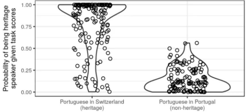
I fitted a random forest of 2,000 trees using the randomForest package (Liaw & Wiener, 2002) for R (R Core Team, 2017). For each tree, the dataset was resampled with replacement and consisted of 134 cases each from the heritage and non-heritage classes. The mtry parameter was set at 2, but setting it to 1 or 3 does not substantially affect the results.
Figure 5 shows the OOB probabilities with which a child is labeled as a heritage speaker, split up by their actual class. If one were to apply a 50% cut-off, 31 out of 171 (18%) heritage speakers would be classified as non-heritage-like, while 2 out of 134 (1.5%) control speakers would be flagged as heritage-like. The miss rate for non-heritagelikeness, then, would be 1.5% (95% CI: [0.4%, 5.3%]). But the probabilities in Figure 5 also underscore that different cut-offs would yield different error rates. On the basis of a 60% cut-off for non-heritagelikeness, for instance, the miss rate would be 0/134 = 0% (95% CI: [0.0%, 2.8%]), but now 36/171 = 21% of the heritage speakers would be categorized as non-heritagelike. In fact, regardless of the cut-off 373 374 375 376 377 378 379 380 381 382 383 384 385 386 387 388 389 390 391 392 393
used (if one is used at all), even the heritage speakers that are classified as heritage-like have some (often non-negligible) probability of being non-heritagelike, and vice versa.
Figure 5. The ‘heritagelikeness’ probabilities that the random forest assigns to each speaker depending on whether the speaker actually was or was not a heritage language speaker.
Discussion and conclusion
I have argued that current estimates of the proportion of L2 speakers that are nativelike according to some set of criteria are difficult to interpret because they are not presented alongside an estimate of the proportion of L1 speakers that would fail to meet the same set of criteria. This latter proportion, the criteria’s miss rate, can be substantial and highlights the possibility that some L2 speakers labeled as non-nativelike may be nativelike after all. This is the case even with L1 control samples that are considerably larger than what is typically found in the literature, particularly when the participants are tested on an entire battery of tasks. I have suggested two ways—there may be more—for estimating a nativelikeness study’s miss rate: collecting data from additional L1 speakers to assess how many of them fail to meet the study’s original
nativelikeness criteria, or reanalyzing the study’s data using a classification model and obtaining 394 395 396 397 398 399 400 401 402 403 404 405 406 407 408 409
its miss rate estimate. Crucially, these approaches assume that the participant samples and the task battery were appropriately constructed—they are not a panacea for biased data.
Classification models that output classification probabilities rather than classifications pure and simple naturally underscore that it may be difficult to state categorically whether an L2 speaker is nativelike or not given the data at hand. Some theoretical approaches conceive of nativelikeness as a binary phenomenon (i.e., L2 speakers either are or are not nativelike, they are not nativelike to varying degrees; cf. Hyltenstam and Abrahamsson’s [2003] ‘non-perceivable non-nativeness’ approach, and some versions of the critical period hypothesis for second
language acquisition, e.g., Long [1990]), and the use of classification probabilities is not at odds with such a theoretical stance. However, even if nativelikeness is a binary phenomenon, lack of data quantity or quality may make it impossible to assess which category a given L2 speaker falls into.
References
Abrahamsson, N. (2012). Age of onset and nativelike L2 ultimate attainment of morphosyntactic and phonetic intuition. Studies in Second Language Acquisition, 34, 187–214.
doi:10.1017/S0272263112000022
Abrahamsson, N., & Hyltenstam, K. (2009). Age of onset and nativelikeness in a second
language: Listener perception versus linguistic scrutiny. Language Learning, 59, 249–306. doi:10.1111/j.1467-9922.2009.00507.x 410 411 412 413 414 415 416 417 418 419 420 421 422 423 424 425 426 427 428
Andringa, S. (2014). The use of native speaker norms in critical period hypothesis research. Studies in Second Language Acquisition, 36(3), 565–596.
doi:10.1017/S0272263113000600
Birdsong, D. (2005). Interpreting age effects in second language acquisition. In J. F. Kroll & A. M. B. De Groot (Eds.), Handbook of bilingualism: Psycholinguistic approaches (pp. 109– 127). New York: Oxford University Press.
Birdsong, D. (2007). Nativelike pronunciation among late learners of French as a second language. In O.-S. Bon & M. J. Munro (Eds.), Language experience in second language speech learning: In honor of James Emil Flege (pp. 99–116). Amsterdam: Benjamins. Birdsong, D., & Gertken, L. M. (2013). In faint praise of folly: A critical review of
native/non-native speaker comparisons, with examples from native/non-native and bilingual processing of French complex syntax. Language, Interaction and Acquisition, 4(2), 107–133. doi:10.1075/lia.4.2.01bir
Birdsong, D., & Molis, M. (2001). On the evidence for maturational constraints in second-language acquisition. Journal of Memory and Language, 44, 235–249.
doi:10.1006/jmla.2000.2750
Birdsong, D., & Vanhove, J. (2016). Age of second-language acquisition: Critical periods and social concerns. In E. Nicoladis & S. Montanari (Eds.), Bilingualism across the lifespan: Factors moderating language proficiency (pp. 163–181). Berlin, Germany: De Gruyter Mouton; American Psychological Association. doi:10.1037/14939-010
429 430 431 432 433 434 435 436 437 438 439 440 441 442 443 444 445 446 447 448
Bongaerts, T. (1999). Ultimate attainment in L2 pronunciation: The case of very advanced late L2 learners. In D. Birdsong (Ed.), Second language acquisition and the critical period hypothesis (pp. 133–159). Mahwah, NJ: Lawrence Erlbaum.
Breiman, L. (2001). Statistical modeling: The two cultures. Statistical Science, 16(3), 199–231. doi:10.1214/ss/1009213726
Bylund, E., Abrahamsson, N., & Hyltenstam, K. (2012). Does first language maintenance hamper nativelikeness in a second language? Studies in Second Language Acquisition, 34, 215-241. doi:10.1017/S0272263112000034
Cook, V. J. (1992). Evidence for multicompetence. Language Learning, 42, 557–591. doi:10.1111/j.1467-1770.1992.tb01044.x
Coppieters, R. (1987). Competence differences between native and near-native speakers. Language, 63, 544–573. doi:10.2307/415005
Davies, A. (2003). The native speaker: Myth and reality. Clevedon, UK: Multilingual Matters.
Dąbrowska, E. (2012). Different speakers, different grammars: Individual differences in native language attainment. Linguistic Approaches to Bilingualism, 2(3), 219–253.
doi:10.1075/lab.2.3.01dab
Desgrippes, M., Lambelet, A., & Vanhove, J. (2017). The development of argumentative and narrative writing skills in Portuguese heritage speakers in Switzerland (HELASCOT project). In R. Berthele & A. Lambelet (Eds.), Heritage and school language literacy 449 450 451 452 453 454 455 456 457 458 459 460 461 462 463 464 465 466 467
development in migrant children: Interdependence or independence? (pp. 83–96). Bristol, UK: Multilingual Matters. doi:10.21832/BERTHE9047
Díaz, B., Mitterer, H., Broersma, M., & Sebastián-Gallés, N. (2012). Individual differences in late bilinguals’ L2 phonological processes: From acoustic-phonetic analysis to lexical access. Learning and Individual Differences, 22, 680–689.
doi:10.1016/j.lindif.2012.05.005
Flege, J. E., Munro, M. J., & MacKay, I. R. A. (1995). Factors affecting strength of perceived foreign accent in a second language. Journal of the Acoustical Society of America, 97, 3125–3134. doi:10.1121/1.413041
Flege, J. E., Yeni-Komshian, G. H., & Liu, S. (1999). Age constraints on second-language acquisition. Journal of Memory and Language, 41, 78–104. doi:10.1006/jmla.1999.2638
Grosjean, F. (1989). Neurolinguists, beware! The bilingual is not two monolinguals in one person. Brain and Language, 36, 3–15. doi:10.1016/0093-934X(89)90048-5
Hopp, H., & Schmid, M. S. (2013). Perceived foreign accent in L1 attrition and L2 acquisition: The impact of age of acquisition and bilingualism. Applied Psycholinguistics, 34(2), 361– 394. doi:10.1017/S0142716411000737
Huang, B. H. (2014). The effects of age on second language grammar and speech production. Journal of Psycholinguistic Research, 43, 397–420. doi:10.1007/s10936-013-9261-7 468 469 470 471 472 473 474 475 476 477 478 479 480 481 482 483 484 485
Hyltenstam, K., & Abrahamsson, N. (2003). Maturational constraints in. In C. J. Doughty & M. H. Long (Eds.), The handbook of second language acquisition (pp. 539–588). Malden, MA: Blackwell.
Johnson, J. S., & Newport, E. L. (1989). Critical period effects in second language learning: The influence of maturational state on the acquisition of English as a second language.
Cognitive Psychology, 21, 60–99. doi:10.1016/0010-0285(89)90003-0
Kuhn, M., & Johnson, K. (2013). Applied predictive modeling. New York: Springer. doi:10.1007/978-1-4614-6849-3
Laufer, B., & Baladzhaeva, L. (2015). First language attrition without second language
acquisition: An exploratory study. International Journal of Applied Linguistics, 166(2), 229–253. doi:10.1075/itl.166.2.02lau
Liaw, A., & Wiener, M. (2002). Classification and regression by randomForest. R News, 2(3), 18–22.
Long, M. H. (1990). Maturational constraints on language development. Studies in Second Language Acquisition, 12, 251–285. doi:10.1017/S0272263100009165
Long, M. H. (2005). Problems with supposed counter-evidence to the critical period hypothesis. International Review of Applied Linguistics in Language Teaching, 43, 287–317.
doi:10.1515/iral.2005.43.4.287 486 487 488 489 490 491 492 493 494 495 496 497 498 499 500 501 502 503
Ortega, L. (2013). SLA for the 21st century: Disciplinary progress, transdisciplinary relevance, and the bi/multilingual turn. Language Learning, 63(Supplement 1), 1–24.
doi:10.1111/j.1467-9922.2012.00735.x
Patkowski, M. S. (1980). The sensitive period for the acquisition of syntax in a second language. Language Learning, 30, 449–472. doi:10.1111/j.1467-1770.1980.tb00328.x
Pestana, C., Lambelet, A., & Vanhove, J. (2017). Reading comprehension development in Portuguese heritage speakers in Switzerland (HELASCOT project). In R. Berthele & A. Lambelet (Eds.), Heritage and school language literacy development in migrant children: Interdependence or independence? (pp. 58–82). Bristol, UK: Multilingual Matters. doi:10.21832/BERTHE9047
R Core Team. (2017). R: A language and environment for statistical computing. R Foundation for Statistical Computing. Software, version 3.4.2. Retrieved from
http://www.r-project.org/
Strobl, C., Malley, J., & Tuz, G. (2009). An introduction to recursive partitioning: Rationale, application, and characteristics of classification and regression trees, bagging, and random forests. Psychological Methods, 14, 323–348. doi:10.1037/a0016973
Tagliamonte, S. A., & Baayen, R. H. (2012). Models, forests, and trees of York English: Was/were variation as a case study for statistical practice. Language Variation and Change, 24(2), 135–178. doi:10.1017/S0954394512000129 504 505 506 507 508 509 510 511 512 513 514 515 516 517 518 519 520 521 522
Van Boxtel, S., Bongaerts, T., & Coppen, P.-A. (2005). Native-like attainment of dummy subjects in Dutch and the role of the L1. International Review of Applied Linguistics in Language Teaching, 43, 355–380. doi:10.1515/iral.2005.43.4.355
Vanhove, J., & Berthele, R. (2017). Testing the interdependence of languages (HELASCOT project). In R. Berthele & A. Lambelet (Eds.), Heritage and school language literacy development in migrant children: Interdependence or independence? (pp. 97–118). Bristol, UK: Multilingual Matters. doi:10.21832/BERTHE9047
523 524 525 526 527 528 529