Determination of the fault plane using a single near-field seismic
station with a finite-dimension source model
D. Legrand1,2 and B. Delouis3
1 Earthquake Research Institute, University of T okyo, 1–1-1 Yayoi, Bunkyo-ku, T okyo 113, Japan. E-mail: [email protected] 2 Maison Franco Japonaise, 3–9-25 Ebisu, Shibuya-ku T okyo 150–0013, Japan. E-mail: [email protected]
3 ET H, Institut fur Geophysik, Honggerberg, CH-8093, Zurich, Switzerland. E-mail: [email protected]
Accepted 1999 May 4. Received 1999 April 10; in original form 1998 December 10
S U M M A R Y
We explore the possibility of determining the actual fault plane of an earthquake from the inversion of near-source displacement seismograms of one station when a finite-dimension source is used instead of a point source model and when the complete displacement is taken into account, including near-field waves. Tests on synthetic seismograms and real data recorded at local distances show that this is possible even with a single, three-component station. A single accelerogram available for the Erzincan, Turkey, 1992 March 13, M
s=6.8 earthquake is inverted and the solution found is compatible with other seismological studies and with the mechanism expected for the North Anatolian Fault.
Key words: earthquake source mechanism, Erzincan earthquake, fault plane solutions,
seismograms, strong ground motion, waveform analysis.
the fault plane with one or few stations, especially when no
I N T R O D U C T I O N
precise aftershock locations or surface rupture is available. The point source approximation is the basic element generally Accelerograms are often used in source studies for their high-used for the inversion of seismic sources. In this case, it is not frequency content (e.g. Spudich & Frazer 1984; Fletcher & possible to identify the actual fault plane from the two nodal Spudich 1998) but are used more rarely for their very low-planes by using waveform modelling. For example, automatic frequency content and/or their static part (e.g. Legrand 1995; determinations of focal mechanisms for teleseismic or regional Delouis et al. 1997; Singh et al. 1997; Courboulex et al. 1997). events (e.g. Buland & Gilbert 1976; Dziewonski et al. 1981; The high-frequency part is usually thought to contain infor-Sipkin 1982, Dreger & Helmberger 1993; Kawakatsu 1995) mation about the complexity of the structure and the dynamics give the seismic moment tensor, but cannot specify the actual of the rupture: it will not be considered in this paper. We will fault plane. In order to select the actual fault plane, additional model only the low-frequency parts of the signals, which information such as the distribution of aftershocks or surface contain information about the fault orientation and the slip ruptures is needed. The approximation of a point source is direction.
generally valid for distances much larger than the size of the fault and the wavelength considered. However, at shorter distances this approximation is no longer appropriate, and the
D E S C R I P T I O N O F T H E P O I N T S O U R C E
finiteness of the source should be taken into account. The A N D F I N I T E - D I M E N SI O N S O U R C E problem of identification of the actual fault plane with a finite
M O D E L S
source model by waveform inversion has already been
con-A physical finite-dimension fault of surface S over which sidered in several studies (e.g. Mori & Hartzell 1990; Dreger
surface forces are applied, generating a dislocation of value D, 1997), but in these works the focal mechanism is fixed in
is mathematically equivalent, in the far field, to a point source advance. Here, we show that the use a finite-dimension source
where two couples of volume forces are applied, each of model (FDSM hereafter) offers the possibility of determining
momentum M
0=mSD (Aki & Richards 1980), where m is the the actual fault plane with little a priori information about the
shear modulus. However, when the source dimension is large focal mechanism, even with data from a single station.
enough relative to the hypocentral distance and to the wave-Accelerographs are well adapted to recording the dynamic
length, the source finiteness will have a strong effect on the and static parts of strong ground motions. However, many
shape of the seismograms (Fig. 1), and must be taken into seismic regions of the world have only sparse strong motion
networks. Hence, it is important to develop methods to identify account.
801
where M
ij=Mij(j=0) is the seismic moment tensor at the pointj=0 and f is the source time function. In that case (1) becomes u n(x, t)=Mij
P
2 −2 dt f (t)g ni,j(0,t; x, t) . (2) The source time function f used in this paper is a ramp function. The duration of the ramp corresponds to the rise time, T , and the final constant value, D, corresponds to the final static displacement on the fault plane (i.e. the dislocation D).In the case of an FDSM, (1) becomes u n(x, t)=
P
2 −2 dtPP
S dj 1dj2Mij(j, t)gni,j(j, t; x, t) , (3) where j=(j1,j2) is the vector position describing the fault surface S.
In this paper, we will consider the simple case where the source time function f is the same at each point of the fault. Thus, we separate the spatial and temporal aspects of the source. With this simple assumption, (3) becomes
u n(x, t)=Mij
P
2 −2 dt f (t)PP
S dj1dj2g ni,j(j, t; x, t) . (4) Eqs (2) and (4) differ in the integration over the fault plane of surface S, and we show in this paper that this difference allows the selection of the fault plane if (4) is used instead of (2). Some caution is warranted in computing eq. (4). It is a joint integration in space and time which is approximated by a discrete summation of N point sources. As a consequence, the temporal and spatial sampling rates cannot be chosen independently (see the Appendix).For the sake of simplicity, in this paper ‘near field’ (NF) means simply that the amplitude of NF waves are not negligible with respect to the amplitude of the far-field waves for the wavelength considered. As mentioned by Vidale et al. (1995) and Cummins (1997), NF waves can be clearly seen in some cases at teleseismic distances (20°–30°) for large earthquakes.
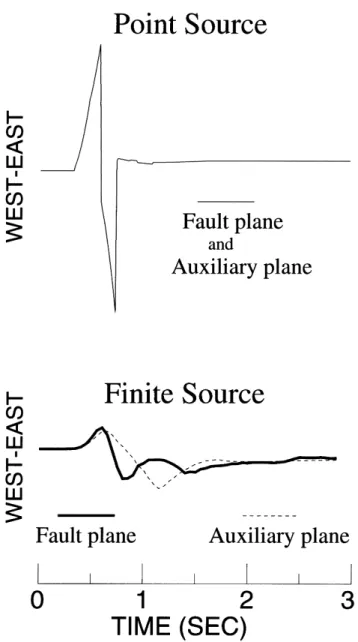
Figure 1. Comparison of a seismogram for a point source (top) an a finite-dimension source model (bottom). The fault plane is
D I S C R I M I N AT I O N O F T H E FA U LT PL A N E
(strike, dip, rake)=(200, 70, 130) and the auxiliary plane is (312, 44, 29).
F O R A F I N I T E -D I ME N S I O N S O U R C E
The hypocentre is at 2 km depth and the epicentral distance is 1 km.
M O D E L W I T H A S I N G L E S TAT I O N
For the FDSM, the nucleation point is at the centre of a 3 km×3 km
fault, the rupture front is circular and the constant rupture velocity is In the case of a point source, M
ijand the spatial derivatives 2.5 km s−1. The rise time is 0.15 s.
of the Green’s functions, g
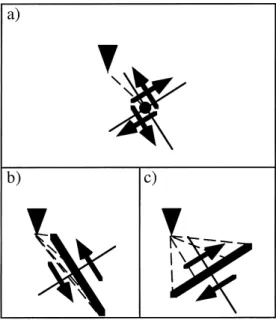
ni,j, with respect to the source coordinates are the same, independent of which of the two nodal planes is the fault plane. The unique path of the g
ni,jin that case is illustrated in Fig. 2(a). Hence, the seismograms For a point source situated atj=0, the displacement u
n(x, t) corresponding to the two nodal planes will be identical calculated at x and at time t is given by the representation
(Fig. 1, top). theorem (Burridge & Knopoff 1964; Aki & Richards 1980),
In the case of an FDSM, M
ijis also the same for the two nodal planes, but now g
ni,jare different. In eq. (4), gni,j corre-u
n(x, t)=
P
2 −2dtMij(0,t)gni,j(0,t; x, t) , (1)
spond to the spatial derivatives of the Green’s functions for all the paths between the surface S and the station considered. where g
ni is the Green’s function tensor corresponding to a Since the orientations of the actual fault plane and the auxiliary displacement in the n direction due to a unit force in the i
plane are different, the corresponding paths of g
ni,jdiffer, as direction and g
ni,j(0,t; x, t)=[∂gni(j=0, t; x, t)]/∂jj are the shown in Figs 2(b) and (c). Consequently, the seismograms spatial derivatives with respect to the source coordinatesj.
corresponding to the actual fault plane and the auxiliary plane For a point source atj=0, the seismic moment tensor can
will be different (Fig. 1, bottom). This difference in the wave-be written as:
forms of the seismograms will allow for the selection of the actual fault plane, as shown below.
M
front with a constant velocity and a constant dislocation over a rectangular fault. We took a nucleation point at the centre of the fault. The influence of the position of the hypocentre, controlling part of the history of the rupture, is important for modelling large earthquakes, but will not be considered here. The influence of the position of the nucleation point is discussed in more detail in Delouis & Legrand (1999).
We perform waveform modelling of body and surface waves in the time domain using a Monte Carlo inversion in order to find the orientation of the fault plane (strike and dip) and the direction of the slip vector on this fault (rake). The selection criterion in the Monte Carlo inversion is the normalized rms error ( hereafter simply called rms) between the observed data (recorded seismograms) and the calculated synthetics. A first series of trials is performed for the entire space of solutions, and several subseries are made around the best solutions of the first series (zoom effect) to define the minimum, better. In order to find out whether we can select the fault plane from the two nodal planes, when a zoom is performed around a solution, we systematically carry out a second zoom around the corresponding auxiliary plane.
Figure 2. Scheme showing the different paths of the Green’s functions (dashed lines) from the source to the station (triangle) for a point source model (a) and an FDSM ( b and c). (a) The unique paths of the
F I R S T S Y N T H E T I C T E S T
Green’s functions for a point source (bold point) does not allow one
to distinguish the fault plane from the auxiliary plane (the two lines). We apply the method with a point source model and with an (b), (c) The different paths from the different points of the fault plane FDSM for a first synthetic example, where the focal mechanism to the receiver allow one to discriminate the fault plane ( bold line is fixed to (strike, dip, rake)=(200°, 70°, 130°). We calculate in b) from the auxiliary plane ( bold line in c).
the corresponding three-component seismograms, called the ‘synthetic data’, which simulate observed data. These ‘synthetic data’ are inverted with the Monte Carlo approach described
ME T H O D O F I N V E R SI O N
above, without adding any noise to the seismograms. The ‘synthetic data’ that we invert are shown for a point We invert NF records using a single three-component
accelero-gram using two models: a point source model and an FDSM. source and for an FDSM in Fig. 1 for the fault plane (strike, dip, rake)=(200°, 70°, 130°) and the auxiliary plane (strike, The spatial derivatives g
ni,jof the Green’s functions are
calcu-lated at the surface of a half-space using Johnson’s (1974) dip, rake)=(312°, 44°, 29°). In this figure, we only show the E–W component for the sake of simplicity.
method, which is based on Cagniard–de Hoop integration
in the time domain. This calculation gives an exact analytic The results of the inversion of the synthetic data are shown for the point source and for the FDSM in Fig. 3. In both cases, representation of the complete displacement field, including NF
waves. In the case of an FDSM, some parameters (the dimen- the original focal mechanism is retrieved. In the case of a point source, the rms values are equal for the two nodal planes, sion of the fault, the dislocation, the rise time and the rupture
velocity) are fixed a priori, because with a single station these hence they cannot be distinguished. This is expected since, as indicated above, the seismograms corresponding to the two parameters cannot be constrained. We use a circular rupture
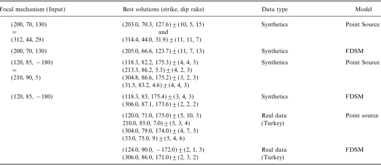
Figure 3. Rms results corresponding to the inversions for the first synthetic test. (Top) For a point source. The two nodal plane cannot be distinguished. (Middle) For an FDSM. The fault plane (strike, dip, rake)=(200°, 70°, 130°) can be distinguished from the auxiliary plane (strike, dip, rake)=(312°, 44°, 29°). (Bottom) Representation of all the 6181 sorts made by the Monte Carlo method.
nodal planes are identical. However, in the case of the FDSM, the synthetic case of Fig. 3 because the calculation of synthetic the rms values corresponding to the two nodal planes are seismograms is time-consuming for such a large source. Hence, significantly different, thus the fault plane can be clearly the uniqueness of the solution is not studied so completely. distinguished from the auxiliary plane, which has been rejected This earthquake is a vertical strike-slip fault. In such a case, by the inversion. This is due to the difference in the correspond- there is an ambiguity of±180° in both strike and rake. This ing seismograms. The results of the inversions are given in means that the solution (strike, dip, rake)=(120°, 85°, −180°) Table 1. The error estimates correspond to solutions having and its auxiliary plane (210°, 90°, 5°) are almost the same as an rms within 10 per cent of the best rms found. that with fault plane (300°, 85°, −180°) and auxiliary plane (30°, 90°, 5°). We carry out a second synthetic test to evaluate the resolution of the method described above for this particular
AP P L I C AT I O N T O T H E E R Z I N C AN
situation. We construct the ‘synthetic data’ with a focal
mech-( T U R K E Y ) E A R T H Q U A K E : S E C O N D
anism (strike, dip, rake)=(120°, 85°, −180°) close to the actual
SY N T H E T I C T E S T A N D I N V E R S I O N O F
solution of the Erzincan earthquake. The first row of Fig. 4 shows
RE A L DATA
the result of the inversion for a point source; four solutions The Erzincan earthquake (1992 March 13, M
s=6.8) occurred can explain the ‘synthetic data’, which are the four triplets along the North Anatolian Fault (Fuenzalida et al. 1997). The
(strike, dip, rake) mentioned above. The second row of Fig. 4 main shock was recorded by a single SMA-1 accelerograph
also shows the solution for an FDSM; now only two solutions located at an epicentral distance of about 10 km.
Trial-and-can explain the ‘synthetic data’, corresponding to the two triplets error modelling of the seismograms, integrated from
accelero-(strike, dip, rake)=(120°, 85°, −180°) and (300°, 85°, −180°) grams, has been carried out by Legrand (1995) and Bernard
mentioned above. Finally, the third and fourth rows of Fig. 4 et al. (1997). Legrand (1995) modelled the three components
show the solution for the Erzincan earthquake for a point to determine the focal mechanism by trial and error, followed
source and an FDSM, respectively. As for the synthetic test, it by a systematic search around the best solution using a simple
is not possible to identify the fault plane with a point source model of propagation. Bernard et al. (1997) modelled the two
model, whereas it is possible to select the fault plane from the horizontal components, taking into account the basin structure,
two nodal planes with an FDSM, because the two possible with a fixed focal mechanism. In this paper we invert the same
solutions found do not correspond to the classical indeter-single three-component seismogram, as a test case for the
minacy between the two nodal planes, but to the ambiguity of method described above, focusing on the selection of the
±180° in both strike and rake mentioned above. The best fault plane.
solution corresponding to an FDSM is (124°, 90°, −172°)± The medium of propagation used is a half-space, with
(2°, 1°, 3°), which is almost the same fault plane as the second V
P=6.0 km s−1 and VS=3.5 km s−1. The size of the fault has minimum found (306°, 86°, 171°)±(2°, 3°, 2°). These solutions been taken as 25 km×10 km, in accordance with the
after-are compatible with the right-lateral strike-slip mechanism of shock distribution and the magnitude. The rise time is 0.7 s
the North Anatolian Fault (Fuenzalida et al. 1997; Bernard and the rupture velocity is Vr=3 km s−1 (Legrand 1995). We et al. 1997). Hence, in the case of the Erzincan earthquake the assume a circular rupture front, initiating at the centre of the
correct fault plane has been automatically selected. The details fault. In the case of Erzincan, the number of trials (5381) in
the Monte Carlo inversion is smaller than the 6181 trials for of the solutions are given in Table 1.
Table 1. Errors are calculated from the standard deviation of the data with an rms smaller than the smallest rms+10 per cent of the smallest rms. Note that the focal mechanism (120°, 85°, ±180°) is almost the same as (300°, 85°, ±180°); see text. The corresponding auxiliary planes are (210°, 90°, 5°) and (30°, 90°, 5°), respectively. FDSM=finite-dimension source model. All values are in degrees.
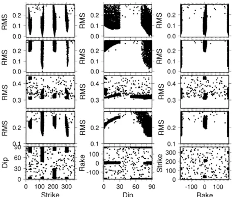
Focal mechanism (Input) Best solutions (strike, dip rake) Data type Model
(200, 70, 130) (203.0, 70.3, 127.6)±(10, 5, 15) Synthetics Point Source
= and
(312, 44, 29) (314.4, 44.0, 31.9)±(11, 11, 7)
(200, 70, 130) (205.0, 66.6, 123.7)±(11, 7, 13) Synthetics FDSM
(120, 85,−180) (118.3, 82.2, 175.3)±(4, 4, 3) Synthetics Point Source
= (213.3, 86.2, 5.3)±(4, 2, 3)
(210, 90, 5) (304.8, 86.6, 175.2)±(3, 2, 3) (31.5, 83.2, 4.6)±(4, 4, 3)
(120, 85,−180) (118.3, 83, 175.4)±(3, 4, 3) Synthetics FDSM
(306.0, 87.1, 173.6)±(2, 2, 2)
(120.0, 71.0, 175.0)±(5, 10, 3) Real data Point source
210.0, 85.0, 7.0)±(5, 3, 4) (Turkey) (304.0, 79.0, 174.0)±(4, 7, 3)
(33.0, 75.0, 9)±(5, 4, 6)
(124.0, 90.0,−172.0)±(2, 1, 3) Real data FDSM
Figure 4. Rms errors for the second synthetic test for a point source model (first row) and an FDSM (second row) for a focal mechanism (strike, dip, rake)=(120°, 85°, −180°). The third and fourth rows correspond to the real Erzincan earthquake data for a point source and an FDSM, respectively. The last row corresponds to the sorts of Monte Carlo methods. A time shift of 0.12 s has been applied on the east component of the Erzincan data because of shear wave splitting observed on the data attributed to anisotropy (Bernard et al. 1997).
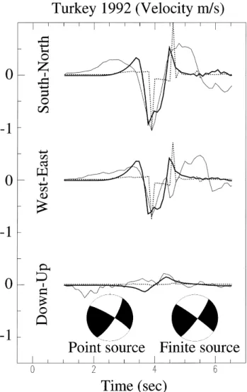
The seismograms corresponding to the best results are With a finite-dimension source model, a more realistic (i.e. shown in Fig. 5 for a point source and an FDSM. The smaller) local rise time can be used. The low frequencies of the dislocation found is 1.5 m, corresponding to a seismic moment calculated seismogram will be naturally generated by the of 1.12×1026 dyn cm for a shear modulus of 3×10¹¹ dyn cm−2. spatial integration over the fault plane (see Fig. 6) and not by increasing the rise time artificially when a point source is used. Although we showed that the recovery of the fault plane
D I S C U S S I O N
with a single station is feasible, we do not imply that it will be NF waves are often omitted in the calculation of synthetic possible in all cases. We cannot exclude the fact that for some seismograms. However, their contribution can be important in specific station–fault geometries the constraint on the fault the case of a point source (see the NF ramp between the P parameter may degenerate.
and S pulses in Fig. 6, top), and extremely important in the The velocity seismogram of the Erzincan earthquake is case of a finite-dimension source (Fig. 6, bottom). Note that surprisingly low frequency, which seems to indicate a relatively NF waves often appear as a ramp for a point source, whereas simple rupture. This justifies the use of a simple model of they often appear as a broad, low-frequency signal for a homogeneous slip. However, for very large earthquakes,
finite source. the rupture may become very heterogeneous, and it should
NF waves decay as 1/r2, whereas the far-field waves decay certainly be taken into account in order to model adequately as 1/r, where r is the radial distance from the source to the the seismograms. Here, a certain degree of heterogeneity may receiver. Hence, a small change in distance implies a larger be invoked to explain part of the misfit in the modelling of change in amplitude of the NF waves than the far-field waves, the second pulse of the Erzincan data. The effect of the and, as a consequence, NF waves provide a sharp constraint Erzincan basin, which we did not take into account, should on the orientation of a finite fault. This property is discussed also explain the misfit of the second pulse. However, the in more detail and has been used to constrain the location method appears to be robust enough, in the sense that this and the focal mechanism of volcanic tremors for a point source misfit did not seem to introduce a significant bias in the by Legrand et al. (1999). estimation of the focal mechanism.
The waveforms of a moderate-sized earthquake may be modelled in the NF with a point source approximation (e.g. Singh et al. 1997; Schwartz 1995; Fan & Wallace 1991). In this
C O N C L U S I O N S
case, the rise time has to be adjusted to the width of the
The actual fault plane can be determined, with little a priori observed waveform pulses. This leads to a long rise time which
information on the focal mechanism, by waveform modelling, measures the total rupture duration of the faulting. It is longer
Figure 5. Result of the modelling of the three-component Erzincan seismogram (fine line) for a point source model (dotted line) and an FDSM ( bold line), with the corresponding focal mechanism ( lower-hemisphere, equal-area projection).
point source and if NF waves are taken into account in the calculation of Green’s functions. With a single station, some of the source parameters such as the fault dimension, the rise time and the rupture velocity cannot be solved and have to be fixed a priori in the inversion. As a consequence, the knowledge of the source can be greatly improved not only by increasing the number of stations (as is often done) but also by considering
Figure 6. Vertical displacement for a pure strike-slip mechanism
FDSMs and using NF waves.
recorded at station A. The rupture propagates towards A. N is the The method of selection of the fault plane from the two
number of point sources. An FDSM is well described by at least 400 nodal planes described in this paper has been applied to local
point sources. See text for more details. The rupture front here is earthquakes but can be applied identically to regional and
taken as linear and unilateral, in the sense shown by the arrow at the teleseismic events (especially for large earthquakes). This study bottom of the figure, the rupture velocity being 3 km s−1. The size of points out the importance of low-frequency modelling in the the fault is 4 km×4 km and the coordinates of A are (3 km N, 0.1 km E); NF. These low frequencies have two origins. First, NF waves Dt=0.02 s. Vertical scale in arbitrary units, depending on the value of are low frequency by nature. Second, the spatial and temporal the dislocation D, which is the same for all of this figure.
finiteness of the source generate low frequencies. Hence, the
use of accelerographs and/or broad-band stations in the NF We have shown that in the case of the Erzincan (Turkey) is crucial for recording the static part and/or the low-frequency earthquake, the fault plane can be distinguished from the two signal in order to constrain the fault plane orientation and the nodal planes with records from a single station when an FDSM and NF waves are used. The selected fault plane slip vector.
Mori, J. & Hartzell, S., 1990. Source inversion of the 1988, Upland, corresponds to the orientation of the North Anatolian Fault,
California earthquake: determination of a fault plane for a small and the focal mechanism is right-lateral strike slip, as expected
event, Bull. seism. Soc. Am., 80, 507–518. for the North Anatolian Fault.
Schwartz, S.Y., 1995. Source parameters of aftershocks of the 1991 Costa Rica and 1992 Cape Mendocino, California, earthquake from inversion of local amplitude ratios and broadband waveforms, Bull.
A C K N O WL E D G M E N T S
seism. Soc. Am., 85, 1560–1575.
Singh, S.K., Pacheco, J., Courboulex, F. & Novelo D.A., 1997. Source We would like to thank the French Ministe`re des Affaires
parameters of the Pinotepa Nacional, Mexico, earthquake of 27 Etrange`res and ETH Zurich for their support, and
March, 1996 (Mw=5.4) estimated from near-field recordings of a Prof. Kawakatsu for his hospitality towards DL. We are grateful
single station, J. Seism., 1, 39–45. to two anonymous reviewers for their critical comments of the
Sipkin, S., 1982. Estimation of earthquake source parameters by the manuscript.
inversion of waveform data: synthetic waveforms, Phys. Earth planet. Inter., 30, 242–259.
Spudich, P. & Frazer, L., 1984. Use of ray theory to calculate
RE F E R E N C E S
high-frequency radiation from earthquake sources having spatially variable rupture velocity and stress drop, Bull. seism. Soc. Am., 9, Aki, K. & Richards, P., 1980. Quantitative Seismology: T heory and
2061–2082. Methods, W. H. Freeman, New York.
Vidale, J.E., Goes, S. & Richards, P.G., 1995. Near-field deformation Bernard, P., Gariel, J.C. & Dorbath, L., 1997. Fault location and
seen on distant broadband seismograms, Geophys. Res. L ett., 22, 1–4. rupture kinematics of the magnitude 6.8, 1992 Erzincan earthquake,
Turkey, from strong ground motion and regional records, Bull. seism. Soc. Am., 87, 1230–1243.
Buland, R. & Gilbert, F., 1976. Matched filtering for the seismic A P P E N D I X A : P R O B L E M OF T H E moment tensor, Geophys. Res. L ett., 3, 205–206.
S PAT I O – T E M PO R A L I N T E G R AT I O N O N A
Burridge, R. & Knopoff, L., 1964. Body force equivalents for seismic
FA U LT P L A N E
dislocations, Bull. seism. Soc. Am., 54, 1875–1888.
Courboulex, F., Santoyo, M.A., Pacheco, J.F. & Singh, S.K., 1997. The A finite-dimension source can be modelled by a superposition 14 September 1995 (M=7.3) Copala, Mexico, earthquake: a source of point sources located on the fault plane at j=(j
1,j2), study using teleseismic, regional, and local data, Bull. seism. Soc. performing the continuous spatial integral (4) by a discrete Am., 87, 999–1010.
spatial summation of N point sources. As the representation Cummins, P., 1997. Earthquake near-field and W phase observations
theorem deals with an integration in both time and space, the at teleseismic distances, Geophys. Res. L ett., 24, 2857–2860.
temporal and spatial samplings cannot be chosen independently, Delouis, B. & Legrand, D., 1999. Focal mechanism determination and
but must verify some conditions of sampling such as those identification of the fault plane of earthquakes using only one or
described by Hartzell et al. (1978). The spatial sampling two near source seismic recordings, Bull. seism. Soc. Am., submitted.
Delouis, B. et al., 1997. The Mw=8.0 Antofagasta (Northern Chile) described by Hartzell, if applied as a limit, is in practice not earthquake of 30 July 1995: a precursor to the end of the large 1877 small enough, so some artificial high frequencies are generated. gap, Bull. seism. Soc. Am., 87, 427–445. We proceed empirically. First, the time sampling is chosen for Dreger, D., 1997. The large aftershocks of the Northridge earthquake a point source. It must be small enough to describe all the and their relationship to mainsshock slip and fault-zone complexity, wavelengths considered in the seismogram and to sample the Bull. seism. Soc. Am., 87, 1259–1266.
rise time correctly, but not too small, in order to avoid high-Dreger, D. & Helmberger, D., 1993. Determination of source
para-frequency noise of numerical origin. When the time sampling meters at regional distances with single station or sparse network
for a point source is chosen, the spatial sampling is determined data, J. geophys. Res., 98, 8107–8125.
as follows. It is reduced until the seismogram reaches a stable Dziewonski, A., Chou, T. & Woodhouse, J., 1981. Determination of
form. The spatial sampling must not be too large, otherwise earthquake source parameters from waveform data for studies of
global and regional seismicity, J. geophys. Res., 86, 2825–2852. high frequencies are generated due to the sampling rate con-Fan, G. & Wallace, T., 1991. The determination of source parameters dition described by Hartzell et al. (1978) not being respected, for small earthquakes from a single, very broadband seismic station, or too small, because in that case it is time-consuming and Geophys. Res. L ett., 18, 1385–1388. high frequencies due to numerical effects are also generated. Fletcher, J. & Spudich, P., 1998. Rupture characteristics of the three This procedure is illustrated in Fig. 6, for which a finite-sized
M~4.7 (1992–1994) Parkfield earthquakes, J. geophys. Res., 103,
fault plane has been modelled with N=1, 4, 16, 64, 400 and 835–854.
1600 point sources. If too small a number of point sources is Fuenzalida, H. et al., 1997. Mechanism of the 1992 Erzincan earthquake
used in the summation, high frequencies arise ( like for N=4, and its aftershocks, tectonics of the Erzincan basin and decoupling
16, 64) due to the space–time samplings not being respected. on the North Anatolian Fault, Geophys. J. Int., 129, 1–28.
We see that 400 point sources is almost enough to describe Hartzell, H., Frazier, G. & Brune, J., 1978. Earthquake modeling in a
homogeneous half-space, Bull. seism. Soc. Am., 68, 301–316. the finiteness of the source. Note the large difference between Johnson, L., 1974. Green’s function for Lamb’s problem, Geophys. the signals from a point source and from a finite-dimension J. R. astr. Soc., 37, 99–131. source. For a point source, positive and negative parts of the Kawakatsu, H., 1995. Automated near-realtime CMT inversion, signal exist, whereas for a finite source, only a positive signal
Geophys, Res, L ett., 21, 1963–1966.
remains. A finite-dimension source contains many more low Legrand, D., 1995. Study of a population of tectonic and volcanic
frequencies than a single point source. For example, the P earthquakes in near-field: from classical seismology to non linear
and S waves which have a form similar to a Dirac distribution effects, PhD thesis, University of Strasbourg (in French).
almost disappear in the case of a finite source; P and S waves Legrand, D., Kaneshima, S. & Kawakatsu, H., 1999. Moment tensor
cannot be distinguished for a finite-dimension source, whereas analysis of near-field broadband waveforms at Aso volcano, Japan,
partly generated by the constructive and destructive inter- by the rise time, which is the time taken for each point of the fault to reach the final dislocation D (the static displacement). ference of waves, especially NF waves. It is a well-known fact
that a large earthquake generates more low frequencies than For a point source, this rise time governs the width of the far-field P and S waves (see Fig. 6, for N=1), whose forms are a small earthquake. Note also that we focus on the effect of
the finiteness in space introduced by the length and width of similar to Dirac pulses as mentioned above. Fig. 6 shows the effect of this rise time during the summation process. the fault, but a similar effect also exists in time, introduced