Determining the rate of change in a mixed deciduous forest monitored for 50 years

ORIGINAL PAPER

Determining the rate of change in a mixed deciduous forest

monitored for 50 years

Annett Wolf

Received: 28 May 2010 / Accepted: 7 October 2010 / Published online: 4 May 2011 # INRA and Springer Science+Business Media B.V. 2011

Abstract

& Introduction Trees in two compartments of the mixed

deciduous forest Draved Forest have been monitored regularly for 50 years.

&Materials and methods This data set was used to study

the rate of change in forest structure and composition applying the Kolmogorov–Smirnov statistics, chi-square test for the goodness of fit, and principal component analysis. We also correlated the specific test statistics with other forest properties to elucidate the importance of various factors for the observed changes in forest structure.

&Results After 50 years, the still significant changes in the

forest structure and species composition indicate that the compartments have not reached the state of an old growth forest. Although some measures indicated that the compart-ments were approaching this stage, other showed the opposite response and even an increasing rate of change.

&Conclusion As the three statistical methods contributed

in different ways, we recommend the combination of several statistical methods to assess changes in the forest structure.

Keywords Long-term monitoring . Diameter distribution . Species composition . Kolmogorov–Smirnov test . Chi-square test for goodness of fit

1 Introduction

Almost all current European forest reserves were

man-aged in the past (Peterken 1996). To estimate how long

these anthropogenic influences will be important and at which point in time they can be negligible compared to natural disturbances, it is necessary to study the rates and directions of change in the forest structure over long time scales. The rates of change in natural forests depend on species composition, establishment, growth, and mortality rate of the different species. Moreover, the type, frequen-cy, and intensity of the disturbance, e.g., wind, fire, avalanches, or flooding and the sensitivity of the present trees to such disturbances influence the rate of change in forest structure and composition. As all of these factors are connected by complex interactions, large data sets are required for the adequate descriptions of these complex systems. Furthermore, if long-lived organisms like trees are involved, short-term studies may give detailed infor-mation, but extrapolation is often problematic and the long-term consequences can generally not be predicted

(Tilman1989; Magnuson1990). A detailed description of

forest structures will help understand natural forest processes and provide a scientific basis for the manage-ment of nature reserves and the justification of their status. It will also facilitate the development of tools for ecologically based management decisions (Christensen

and Emborg 1996; Bengtsson et al. 2000; Farrell et al.

2000; Führer2000).

Natural forests in Europe (Peterken 1996) are rare,

though significant studies have been carried out in

Bialowieza, Poland (Falinski 1986; Bernadzki et al.

1998), but the forest clearly showed evidence of past

Handling Editor: Matthias Dobbertin

A. Wolf (*)

Forest Ecology, ETH Zurich, ETH-Zentrum, CHN, G77, Universitätsstr. 16,

8092 Zurich, Switzerland e-mail: [email protected] DOI 10.1007/s13595-011-0066-2

human influence (Mitchell and Cole 1998). The Danish forest Suserup has been studied intensively (Christensen et

al.1993; Emborg et al. 2000), but also here, pollen and

macrofossil analyses clearly showed anthropogenic

influ-ences (Hannon et al.2000). Further interesting studies of

old growth forests in England (Peterken and Jones1987;

Mountford et al.1998; Mountford et al. 1999) and forests

reserves in Switzerland (Heiri et al. 2009) showed clear

signs of human influence. It becomes clear that history is of great importance for forest structure and development

(Woods2000), and it is therefore important to know after

which time human influences are not noticeable anymore. Although forest ecosystems have been described in many

studies (for example Leibundgut 1993; Korpel' 1995;

Peterken 1996; Commarmot et al. 2005), the temporal

aspect is often descriptive (illustrated by diagrams and figures) while statistical analysis of these changes are lacking.

Natural forests consist of a mosaic of sequential phases: gaps, regeneration stage, growth phases, mature

and aging phase (e.g., Korpel'1995; Emborg et al.2000;

Kimmins 2004), whereby the areas occupied by these

stages can have varying sizes depending on the forests and the disturbance regimes. If the forest area is large enough, so that all stages can be represented, the forest as a whole can reach an equilibrium stage, where fluctuations in, e.g., biomass or species composition are low and hence changes in these forest characteristics are slow. It is important to notice that the size of the dominant disturbances determine the area over which the forest can

be seen as stable (Korpel'1995); even a smaller forest can

maintain all phases of the forest mosaic if small-scale wind disturbances are dominating, as shown for the

Danish forest Suserup (Emborg et al.2000).

In the context of climatic change, it is important to quantify the rate of change of forest properties such as biomass and species composition as they have a direct influence on the forest carbon storage and hence determine whether we can expect that forests are carbon sources/sinks

or if little changes will occur (Wirth et al. 2009).

Additionally, if rates of change would be known for many decades or even centuries, current rates of change could help to assess whether forest ecosystems can cope with environmental changes and if ecosystem goods and services might still be provided in the future.

In this study, we aim to analyze statistically the temporal changes of a number of forest characteristics, such as diameter distribution, species composition, and biomass, whereas other descriptive parameters considering

biodiver-sity or spatial structure (Neumann and Starlinger2001) are

outside the scope of this study.

We will compare a number of statistical methods and test their similarities and differences when analyzing the rate of

change in forest structure in Draved Forest, a semi-natural

deciduous forest in Denmark (Møller 2000; Wolf 2003;

Bradshaw et al. 2005). We correlate the results with other

forest properties, such as the basal area, mean diameter increment, the number of new established or dead trees, and the change in tree numbers, to help in interpreting them. Finally, we quantify the speed of the development of the forest Draved Forest and compare the results of the different statistical methods.

2 Method 2.1 Draved Forest

Draved Forest (55°01′ N, 8°58′ E) is a mixed deciduous

forest in southwest Jutland, Denmark. Two parts of the forest have been left unmanaged since 1952 (Lime compartment, 4.4 ha) and 1948 (Carlsberg compartment, 5.3 ha). In the pollen diagrams of the Lime compartment, little pollen of grasses and light-demanding species were found, indicating uninterrupted tree cover and the absence or the low intensity of grazing before beech

arrived in the area (Iversen 1958; Bradshaw et al.2005).

It is therefore likely that the wetter areas of Draved Forest

remained largely unmanaged (Iversen1958). Additionally,

Iversen (1958) concluded that the Lime compartment has a

relict character as the pollen in the upper soil layer (around 1950) were identical with the older pollen layers, both for trees and ground vegetation. The few written accounts of the forests make it difficult to assess the past management

directly (Aaby 1983; Møller 2000; Wolf 2003). The

forest’s relative remote location within the wetlands and

mires until recent times (Iversen 1958) together with the

low number of written accounts indicate that forest

management was not intensive (Iversen 1958). Although

few reports of management exist before the eighteenth century, grazing in the forest, mainly by cows, but also by

horses and pigs (Møller 2000) was mentioned; however,

grazing ceased in 1784/85 (Møller2000; Wolf2003). The

forest management plans of 1839–1863 indicate that parts were managed in stripes and as coppice (35 years) with

standards (100–140 years) (Møller 2000; Wolf 2003).

Already in the management plans of 1886–1905, parts of the forests, e.g., the Lime compartment, were set aside to

allow for free forest development (Møller 2000; Wolf

2003). However, in the 1920s and 1930s, the removal of

dead wood and logs were allowed in these areas (Møller

2000; Wolf 2003), but the stands had still a protective

status, allowing only for moderate thinning to preserve the

forest composition (Møller2000; Wolf2003). From 1800

onward, ditches were built to drain the area, whereby some ditches were closed down until 2000, and the rest has not

been maintained after 2000 (Møller2000). For other parts of the forest, more intensive management has been reported as well, including planting of Picea abies (Aaby

1983). Taken together, it is suggested that in parts of

Draved Forest management was not intensive, especially in stands on the moist brown earth where species

composition hardly changed (Iversen 1958, 1969; Aaby

1983; Møller2000; Møller and Bradshaw2001).

2.2 Disturbances and mortality

In the two compartments, tree mortality is relatively low, with around 5% per decade for trees larger than 100 mm in

diameter at breast height (dbh) (Wolf et al.2004). Wind is

the most important external mortality agent in the forest, being responsible of 50–70% of the mortality (Wolf et al.

2004). Between the 1950s and 2003, about 80% of the

wind-created gaps were single tree gaps (Wolf et al.2004),

resulting in the dominance of small-scale disturbances. Even in the most intensive storm ever observed in Denmark

(DanmarksMeteorologiskeInstitut 1999; Wolf et al. 2004)

only 4–5% of the trees larger than 100 mm in dbh were

wind felled, whereby half of them were uprooted and half of them broken, creating relatively small gaps (Wolf et al.

2004). The remaining dead trees were standing dead trees,

for which the low growth rate and a small tree size prior to death indicated competition as an important mortality factor

for these trees (Wolf et al.2004).

2.3 Forest monitoring

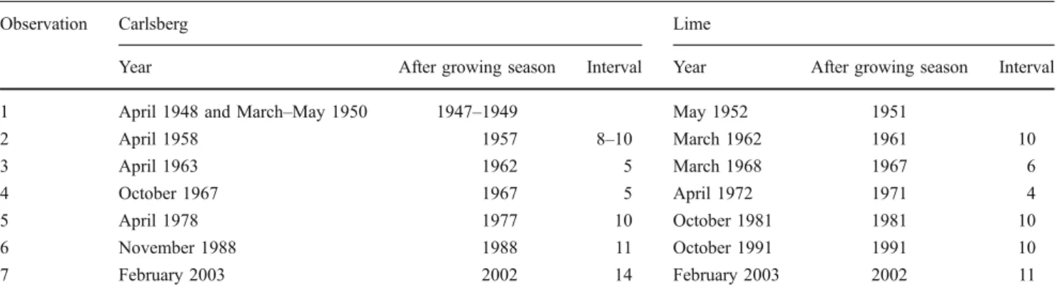
Seven complete surveys were done in the none-growing season, six of them at approximately 10-year intervals, and an intermediate sampling in 1963 and 1968, respectively.

The sampling dates are summarize in Table 1. All trees

larger than 100 mm dbh were identified and measured to the closest millimeter, and their positions were mapped. New recruits, i.e., trees that established into the 100-mm

diameter class, were added to the maps, and dead trees were recorded.

2.4 Changes in species composition

We applied a principal component analysis (PCA) to describe the temporal change in species composition, using the statistic package R (version 2.8.1). The PCA was based on the proportion of the basal area each species contributed to the total basal area. All rare species (less than

0.5 m2 ha−1) were lumped into one class. The results of

the PCA based on the tree numbers per species instead of the basal area were similar and therefore not shown. 2.5 Chi-square test for goodness of fit

The chi-square test for goodness of fit (sometimes called Pearson’s statistics) compares two distributions with each

other (Sokal and Rohlf1995). We calculated the statistics of

the chi-square test using the statistic package R (version 2.8.1), whereby p values where estimated with the Monte Carlo approach (10,000 replicates). Within each compart-ment, we compared each observation with each other. As the chi-square test is based on distinct classes, we divided the data set in diameter classes. Due to the specifics of the chi-square test, all classes need to contain at least one tree,

we therefore defined a class of“reminding trees”, where all

trees were pooled where the size class contained no trees in a least one observation. As this was the case mainly for large trees (ca. 500 mm or larger, depending on species), this pooling means that information on the differences of the larger trees was lost. We rescaled the distributions because for the chi-square test both distributions have to contain the same numbers of trees. This means that the chi-square test compares the distribution, but does not consider differences in the number of trees. To show the dependence of the results on the choice of diameter classes, we present results for three diameter classes (10, 40, and 100 mm).

Table 1 Sampling dates for the observations

Observation Carlsberg Lime

Year After growing season Interval Year After growing season Interval 1 April 1948 and March–May 1950 1947–1949 May 1952 1951

2 April 1958 1957 8–10 March 1962 1961 10 3 April 1963 1962 5 March 1968 1967 6 4 October 1967 1967 5 April 1972 1971 4 5 April 1978 1977 10 October 1981 1981 10 6 November 1988 1988 11 October 1991 1991 10 7 February 2003 2002 14 February 2003 2002 11

2.6 Kolmogorov–Smirnov

The Kolmogorov–Smirnov statistics, D, compares the

good-ness of fit for two distributions (Sokal and Rohlf1995), i.e.,

whether they are significantly different from each other or not. We calculated the value of D using the statistic package R (version 2.8.1). To estimate the significance of the

observed value Dobs, we took random samples (see below)

and derived Drandom. For a p value of 0.05 (one-tailed), Dobs

is larger than Drandom in at least 95% of all such

comparisons. As numbers of trees differed between compart-ments, observations, and species, we applied the randomi-zation procedure for each pair of distributions and used the observed number of trees to constrain the random sampling (see below). We carried out 10,000 randomizations for each

observed pair and estimated the value D95, which is larger

than 95% of all Drandom. To be able to compare the D values

between observations, compartments and species, we

calcu-lated the difference diff.D=Dobs−D95. A value of diff.D

larger than zero indicates that both distributions are significantly different from each other (p≤0.05), whereas a value smaller than zero indicates that the distributions do not differ significantly at this level.

2.7 Sampling of two random distributions

To avoid p values depending on the exact distribution function, we assumed three different functions: uniform, normal, and negative exponential. For each function, we used two different parameter settings, this resulted in six different distribution function from which we sampled randomly. As no systematic differences in p values for the different functions or parameter settings were found,

Drandomfrom all functions were pooled. As the D value of

the Kolmogorov–Smirnov test was sensitive to the number of trees in the two distributions, we maintained the observed numbers of trees when drawing random values from the distribution functions.

3 Results

3.1 Forest properties

The basal area increased in both compartments with time

(Table2), whereby for the last decade the change in basal

area was minor in the Lime enclosure, and the basal area of

the Carlsberg enclosure still increased (Table2). Similarly,

the number of trees increased, and both the number of new trees and the number of dead trees increased through time

(Table 2). The rate of change in tree numbers varied

between observations, and no clear trend could be seen

(Table2).

3.2 Changes in the diameter distributions

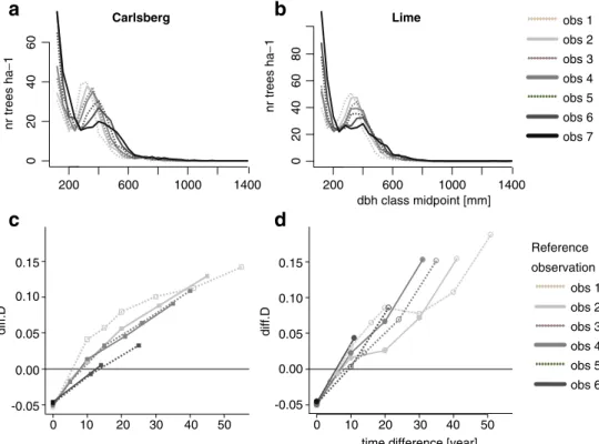
The diameter distributions and their changes through time

are shown in Fig. 1a, b. The distinct peak in the diameter

distribution of the first observations diminished through time and became closer to the negative exponential distribution expected for forests with continuous

recruit-ment (Peterken1996).

The Kolmogorov–Smirnov test was used to measure the rate of change in the diameter distribution, whereby larger values of the test statistic diff.D indicate a larger difference between the two distributions and hence a larger rate of change. This test showed that after about 10 years the diameter distribution has changed significantly in both compartments, independently of the time period considered

(Fig.1c, d). The change in distribution measured with diff.D

increases with the time between the observations; after around 5 years the distributions were not different, but after 10 years most were. In both compartments, the diff.D values increased even further with time, indicating that the differences in the diameter distribution between the two observations increased with increasing temporal distance between observations. In the Carlsberg compartment, the

decadal diff.D values became smaller with time (Table 3),

but four to five data points are too few to describe a trend, especially as the Lime compartment showed no clear

temporal trend of the decadal diff.D (Table3).

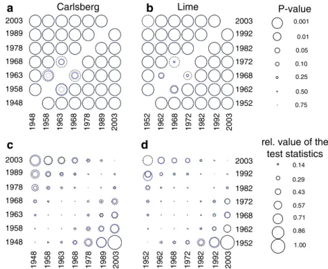
The chi-square test of the goodness of fit is another measure for the rate of change; the larger the test statistics (chi-square value), the larger the difference between the two distributions and consequently the larger the rate of change in the diameter distributions. The chi-square test of goodness of fit showed that all distributions were signifi-cantly different if there were at least 10 years between the

observations (Fig.2a, b). For the three observations that are

only 4–6 years apart, the result depended on the classifi-cation chosen. If the diameter classes were small (10 mm,

dotted lines in Fig. 2), the distributions were significantly

different from each other for all comparisons, except in 1962–1968 (p=0.06). Using larger diameter classes led more often to nonsignificant differences in the 5-year intervals. The more time had passed between the two observations, the more different were the diameter distri-butions, as indicated by the larger differences in the

chi-square values (Fig.2c, d).

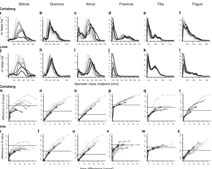
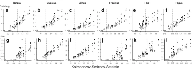
The diameter distribution of the species differed (Fig.3),

whereby species like Betula (Fig. 3a, g) and Quercus

(Fig.3b, h) showed a unimodal distribution with little or no

establishment of trees into the smallest diameter class,

whereas in other species like Fagus (Fig. 3f, l), Tilia

(Fig. 3e, k), and Fraxinus (Fig. 3d, j) trees grew into the

smallest measured diameter class, hence a continuous recruitment occurred. When analyzing the change in the

diameter distribution, communalities were found, but also differences were apparent both within species and

compart-ments (Fig. 3). After about 5 years, none of the species

showed significant changes in diameter distributions. Alnus was the species with the fastest and most consistent changes

in diameter distributions (Fig. 3o, u), as all diameter

distributions for which the observations were at least 10 years apart differed significantly. The notable exception was the last two observations in the Lime enclosure where the diameter distributions did not differ significantly

anymore (Fig.3u). For the other species, the rate of change

in the diameter distribution, as measured with diff.D, was lower, but significant differences were found in the

Carlsberg compartment for most species (Fig. 3m, n, p, q,

r) when at least 20 years had passed between the

observations. However, for the Lime compartment

(Fig.3s–x) the rates of change in the diameter distributions

were somewhat lower compared to the Carlsberg

compart-ment (Fig. 3m–r). The rate of change, as measured with

diff.D, had a clear temporal trend for Betula (Fig. 3m, s),

Quercus (Fig. 3n, t), and Alnus (Fig. 3o, u), resulting in

smaller differences between observations as time pro-gressed. Hence, the diameter distribution changed more between the first observations (higher rate of change) and less between the later ones. The other species did not show

a temporal trend in the diff.D value (Fig. 3p, q, r, v, w),

200 600 1000 1400 02 0 4 0 6 0

time difference [year]

diff.D 0 10 20 30 40 50 0.15 0.10 0.05 0.00 -0.05 200 600 1000 1400 0 2 04 06 08 0 dbh class midpoint [mm] nr trees ha − 1 nr trees ha − 1 Carlsberg Lime 0.15 0.10 0.05 0.00 -0.05 0 10 20 30 40 50 diff.D obs 1 obs 2 obs 3 obs 4 obs 5 obs 6 obs 7 Reference observation obs 1 obs 2 obs 3 obs 4 obs 5 obs 6

a

b

c

d

Fig. 1 Changes in diameter distribution a, b for the two compartments. Different shadings indicate different observations (dates given in Table1). The Kolmogorov– Smirnov statistic diff.D is shown in (c, d), whereby the shadings indicate the reference year. The larger the diff.D value, the larger is the difference in the diameter distribution, and hence the rate of changes between the two observations. The zero line is drawn in black, whereby diff.D values larger than zero indicate a significant difference between the two observations

Table 2 Basal area (square meters per hectare), in parenthesis the change in basal area (square meters per hectare) and number of trees (per hectare) and the change in number of trees in parenthesis (per

hectare) are presented for both compartments and the seven observations (dates are given in Table1)

Observation Basal area (change) [m2ha−1] Number trees (change) [ha−1] New trees [ha−1] Dead trees [ha−1] Carlsberg Lime Carlsberg Lime Carlsberg Lime Carlsberg Lime

1 18.7 (–) 23.5 (–) 240 (–) 314 (–) 2 21.8 (3.1) 27.8 (4.3) 255 (15) 343 (29) 20.0 31.5 4.4 2.3 3 23.5 (1.7) 29.1 (1.3) 270 (15) 340 (−3) 17.5 11.4 2.9 14.2 4 25.1 (1.6) 30.0 (0.9) 282 (12) 340 (0) 17.7 7.5 5.5 8.4 5 27.4 (2.3) 31.1 (1.1) 305 (23) 363 (23) 38.6 45.2 15.6 21.5 6 29.5 (2.1) 32.3 (1.2) 324 (19) 380 (17) 38.4 40.4 20.0 23.5 7 36.2 (6.7) 32.3 (0.0) 326 (2) 412 (32) 48.7 74.2 46.4 42.0

The values in parenthesis indicate the change compared to the previous observation. New trees and dead trees are trees that have reached the 100-mm class or died since the last observation

except for Fagus (Fig.3x) in the Lime compartment where the differences between the two consecutive observations increased with time.

For the diameter distributions of the six main species, the two measurements of the changes in diameter distributions, the chi-square test, and the Kolmogorov–

Smirnov test were well correlated (Fig. 4). This means

that the general features of the change in the diameter distribution were shown by both tests similarly. The chi-square test, however, resulted more often in significant differences between distributions compared with the

Kolmogorov–Smirnov test (Fig.4).

0.001 0.01 0.05 0.10 0.25 0.50 0.75 P-value

rel. value of the test statistics Carlsberg Lime 2003 1992 1982 1972 1968 1962 1952 2003 1992 1982 1972 1968 1962 1952 2003 1992 1982 1972 1968 1962 1952 2003 1992 1982 1972 1968 1962 1952 2003 1989 1978 1968 1963 1958 1948 2003 1989 1978 1968 1963 1958 1948 2003 1989 1978 1968 1963 1958 1948 2003 1989 1978 1968 1963 1958 1948

a

b

c

d

Fig. 2 A comparison of the diameter distribution between the different observations using the chi-square test. Shadings indicate different assumptions about the size of the diameter classes: dotted black, 10 mm; gray, 40 mm; and black, 100 mm. For p values (a, b), a larger circle indicates a high significant difference, whereas a small circle indicates nonsignificant differences. For most comparisons, the

p values are so similar that the lines are drawn over each other. The relative values of the chi-square statistics (c, d) are presented, whereby the larger the circle is the large is the difference in the diameter distribution between the observations and hence the larger the rate of the change in diameter distribution. The sizes are comparable within one shading Compartment Observation 1–2 2–3 3–5 5–6 6–7 All Carlsberg 0.050 0.027 0.003 0.000 na Lime 0.034 0.018 0.026 0.017 0.055 Alnus Carlsberg 0.084 0.055 0.004 0.011 na Lime 0.090 0.076 −0.004 0.017 −0.003 Quercus Carlsberg 0.018 0.022 −0.043 −0.027 na Lime 0.018 0.005 −0.020 −0.045 −0.029 Betula Carlsberg 0.049 0.002 −0.014 −0.081 na Lime 0.007 −0.039 −0.116 −0.137 −0.144 Fagus Carlsberg 0.017 −0.016 0.024 0.008 na Lime −0.055 −0.060 −0.033 −0.027 −0.003 Fraxinus Carlsberg 0.006 0.006 0.091 −0.003 na Lime −0.331 −0.265 −0.187 −0.093 −0.013 Tilia Carlsberg 0.050 −0.056 −0.097 −0.081 na Lime −0.006 −0.020 −0.016 −0.041 −0.017

Table 3 Value diff.Dof the Kolmogorov–Smirnov compari-son of the diameter distributions for two observations

All comparison were made based on observations that were 10 or 11 years apart. The header indicates the two observations that were compared (for dates see Table1). Positive values of diff.D indicate a significant difference between two distri-butions, whereas negative values indicate that the difference was not significant. Values are given for all trees (all) and for indi-vidual tree species

na denotes that data was not available

3.3 Changes in species composition

The compartments showed a distinctive difference in

species composition (Fig. 5) along the first axis (93%

variation explained), whereby the amount of Tilia and Fraxinus distinguished the two compartments. Considering the temporal development, both compartments showed a

similar trend along the second axis of the PCA (Fig. 5),

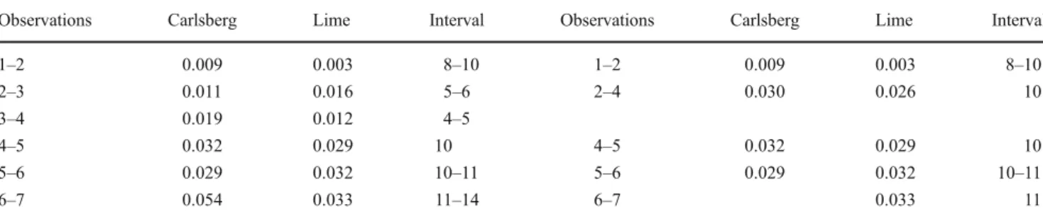
representing an increased importance of Fagus, Alnus, and Quercus and a parallel decrease of Betula. The rate of change in species composition, measured by the Euclidean distance in the PCA, was lower between the first two

observations (Table 4, observations 1–2) than later on

(Fig.5; Table4other observations).

3.4 Correlations between test statistics and forest properties Here, we compared two consecutive observation periods with each other and investigated whether the rate of change in forest attributes, as estimated with the three test statistics, correlated with other forest properties.

The rate of change in species composition (estimated with the Euclidean distance in the PCA) correlated with the number of dead trees, the number of new trees, and the basal area, but not with the average growth or the difference in tree numbers

(Table 5). The rate of change in the diameter distribution

estimated with the chi-square test correlated with the number of new trees and the average growth, but was not correlated with the number of dead trees. The Kolmogorov–Smirnov

200 300 400 500 600 024681 0 1 2 200 400600 800 1200 024 6 8 100 200 300 400 500 600 700 02 4 6 8 1 0 1 2 100 200 300 400 500 600 700 0 5 10 15 20 25 100 300 500 700 02 46 8 200 400 600 800 0 5 10 15 20 200 300 400 500 600 0246 200 400 600 800 1200 02 4 6 8 1 0 100 200 300 400 500 600 700 0 5 10 15 100 200 300 400 500 600 700 02 46 81 0 1 2 1 4 100 300 500 700 01 0 2 0 3 0 4 0 200 400 600 800 0 5 1 01 52 02 53 03 5 nr tr ees ha -1 nr tr ees ha -1 0 10 20 30 40 50 -0 .3 -0 .2 -0 .1 0 .0 0 .1 0 .2 0 10 20 30 40 50 -0 .2 -0 .1 0.0 0 .1 0.2 0 .3 0 10 20 30 40 50 -0 .1 0.0 0 .1 0.2 0 .3 0.4 0 10 20 30 40 50 -0 .6 -0 .4 -0 .2 0 .0 0 .2 0 .4 0 10 20 30 40 50 -0 .2 -0 .1 0.0 0 .1 0.2 0 10 20 30 40 50 -0 .1 0 0 .0 0 0 .10 0 .2 0 0 10 20 30 40 50 -0 .3 -0 .2 -0 .1 0 .0 0 .1 0 .2 0 10 20 30 40 50 -0 .2 -0 .1 0 .0 0 .1 0 .2 0 .3 0 10 20 30 40 50 -0 .1 0.0 0 .1 0.2 0 .3 0.4 0 10 20 30 40 50 -0 .6 -0 .4 -0 .2 0 .0 0 .2 0 .4 0 10 20 30 40 50 -0 .2 -0 .1 0.0 0 .1 0.2 0 10 20 30 40 50 -0.10 0.00 0.10 0.20 di fference in D-value di fference in D-value Quercus Alnus

Betula Fraxinus Tilia Fagus

Carlsberg Lime Carlsberg Lime a b c d e f g h i j k l m n o p q r s t u v w x

diameter class midpoint [mm]

time diff erence [years]

Fig. 3 Changes in diameter distribution for six tree species in the Carlsberg compartment (a–f) and the Lime compartment (g–l). Shadings indicate different observations; for code see Fig.1. Values of the Kolmogorov–Smirnov statistic diff.D for the six tree species for the Carlsberg compartment (m–r) and the Lime compartment (s–x).

The zero line is drawn in black, whereby diff.D values larger than zero indicate a significant difference between the two observations. Shadings indicate the reference year on which the statistic is based upon; for code see Fig.1

test, which also tested the rate of change in the diameter distribution, did not correlate with the number of dead trees, the number of new trees or the average growth in the respective period, but was correlated to the change in tree

numbers (Table5).

4 Discussion

4.1 Forest development

All indicators used here showed that both compartments had high rates of change in species composition and diameter distribution, which indicates that the forest is recovering from past anthropogenic influences after management ceased, even though management might never have been intensive. Strong changes in the diameter distributions were also found in other mixed deciduous forests, where former management was

important (Bernadzki et al. 1998; Mountford et al. 1999;

Heiri et al.2009). When measurements were about 10 years

or more apart, the diameter distributions of all the trees differed significantly in most cases, independent of the statistical method used, whereas after only 5 years, no significant changes in the diameter distribution could be shown when using the Kolmogorov–Smirnov test or the chi-square test with larger diameter classes.

The species composition on the other hand changed more slowly after abandonment, but the rate of change in species composition increased with time, indicating that species turnover increased. This could be mainly attrib-uted to the loss of Betula and an increase in Fagus (both in basal area and tree numbers), especially in the Lime compartment. The importance of Fagus in the species composition and hence the structure of natural deciduous forests are supported by studies throughout Europe (Koop

and Hilgen1987; Ellenberg1996; Peterken1996; Tabaku

1999; Tabaku and Meyer 1999; Emborg et al. 2000;

Meyer,2005). 0.2 0.1 -0.1 -0.2 0.0 0.2 0.1 -0.1 -0.2 0.0 Tilia Fraxinus Betula Fagus Alnus Quercus

temporal change Carlsberg _{temporal change Lime}

axis 1

axis 2

Fig. 5 Temporal change of species composition using PCA. Black dots indicate different observations. The temporal development is indicated by an arrow for both compartments. The species contribu-tions to the different axes were scaled with factor 0.2. The first explains 93% and the second axis 6% of the variation

0.0 0.1 0.2 0 5 10 15 0.0 0.1 0.2 0.3 0 5 10 15 20 25 0.0 0.1 0.2 0.3 0.4 02 0 4 0 6 0 0.0 0.1 0.2 0.3 0.4 0 1 02 03 04 05 0 0.0 0.1 0.2 0 5 10 15 0.00 0.05 0.10 0.15 0.20 0 5 10 15 0.0 0 2 4 6 8 10 12 0.0 0.1 0.2 0.3 05 10 15 0.0 0.1 0.2 0.3 0.4 0 1 02 03 04 0 0.0 0.2 02468 1 0 1 2 0.00 0.04 0 5 10 15 0.00 0.05 0.10 −0.10 −0.10−0.05 −0.08 −0.04 −0.2 −0.1 −0.1 −0.1 −0.1 −0.2 −0.1 −0.1 −0.1 −0.2 −0.1 −0.2 −0.3 −0.6 −0.4 −0.2 0.15 02468 1 0 1 2 1 4 Kolmogorov-Smirnov-Statistic

Betula Quercus Alnus Fraxinus Tilia Fagus

sqr t(Chi-square statistic) sqr t(Chi-square statistic) Carlsberg Lime

a

b

c

d

e

f

g

h

i

j

k

l

Fig. 4 Comparisons of the Kolmogorov–Smirnov statistics with the square root of the chi-square statistic, whereby black dots indicate the chi-square statistic based on diameter classes of 40 mm and gray dots of 100 mm. Empty squares indicate that the chi-square test was not significant, whereas filled circles indicate significant differences. The

dotted line is the vertical zero line. If values for the Kolmogorov– Smirnov statistic (diff.D) are lower than zero, the difference was not significant, whereas values higher than zero indicate a significant difference

When looking at the diameter distribution of the different species, a clear pattern emerged. Some species showed a clear unimodal diameter distribution (Betula, Quercus, and to some degree Alnus) reflecting their

demands of light for establishment (Ellenberg, 1996).

Light-demanding species can only establish in sufficiently large gaps, created naturally (disturbances) or by manage-ment. The observed lack of establishment indicates that not enough areas with sufficient light conditions occurred in the compartments in the past 50 years. The unimodal distribu-tion indicates that such condidistribu-tions were found in the past, favoring the establishment of light-demanding species. Management is the most likely factor to have created these light conditions, as wind disturbances seem to create mainly

small gaps in these compartments (Wolf et al. 2004), and

some past management was reported. Additionally, the temporal development of the spatial pattern of trees also

indicated the influence of past management (Wolf2005). A

similar behavior of light-demanding species has been found

in other forests (Parker et al.1985; Bernadzki et al. 1998;

Mountford et al. 1999; Heiri et al. 2009). The rate of

change in diameter distributions and the variability between observations differed between species. For species with a unimodal diameter distribution (Betula, Quercus, and

Alnus) the rate of change in the distribution decreased continuously, indicating that the differences in the diameter distributions became less distinctive between observations or even disappeared. For Betula, this can be easily explained, as growth rate steadily decreased until the sixth

survey (Wolf, 2003), and hence shifts in diameter

distribu-tions should become less pronounced. Fagus showed the opposite pattern in the Lime compartment, where the continuous increase in number of trees in the smallest size classes was most likely responsible for the increase in the rate of change in the diameter distribution. Interestingly, Tilia had smaller rates of changes in diameter distribution compared to Fagus for example, as it had a lower growth

rate (Wolf2003) and a low mortality (Wolf et al.2004).

4.2 Comparing the different measures of the rates of change Depending on the measures used and the species or compartment analyzed, the rate of changes in diameter distribution differed. We would expect that the rate of change in the diameter distribution should slow down when it approaches the negative exponential distribution expected from natural forests with continuous

regenera-tion (Peterken 1996). There is some indication that the

Table 5 Significant values when the statistic measures (Kolmogorov– Smirnov test, chi-square test, PCA) were correlated (Kendall correlation) with five stand characteristics (number of dead trees,

number of new trees, mean diameter increment, basal area, and change in the number of trees)

Statistical measure Number dead trees Number new trees Mean diameter increment [mm] Basal area Change in tree numbers

Kolmogorov–Smirnov ns ns ns ns **

Chi-square (10) ns *** * ns **

Chi-square (40) ns ** *** ns +

Chi-square (100) ns * ** ns *

Euclidean distance *** ** ns * ns

For the chi-square test results were based on diameter classes of 10, 40, or 100 mm. Euclidean distance represent the distance of observations in the PCA, considering the first and second axis

ns nonsignificant

*p=0.05; **p=0.01; ***p=0.001; +p=0.1

Table 4 Euclidean distance between observations as derived from the first two axes of the PCA

Observations Carlsberg Lime Interval Observations Carlsberg Lime Interval

1–2 0.009 0.003 8–10 1–2 0.009 0.003 8–10 2–3 0.011 0.016 5–6 2–4 0.030 0.026 10 3–4 0.019 0.012 4–5 4–5 0.032 0.029 10 4–5 0.032 0.029 10 5–6 0.029 0.032 10–11 5–6 0.029 0.032 10–11 6–7 0.054 0.033 11–14 6–7 0.033 11

Observation dates given in Table1. Left side of table: values including all observations, right side: Euclidean distance if only observations with 10–11 years temporal difference where considered, i.e., without observation number 3

rate of change in the diameter distribution (measured with the Kolmogorov–Smirnov test) slowed down in the Carlsberg compartment, but not in the Lime compartment. Equally for some species, the rate of change in the diameter distribution declined (Betula, Quercus), but not for the other for which no clear temporal trend was detectable. The basal area still increased in both ments although at a decreasing rate in the Lime compart-ment, which indicates that it might come closer to the maximum basal area for this compartment. The Carlsberg compartment, however, showed a decreasing rate of basal area growth only until the sixth survey, whereas in the last survey the basal area increment was larger again. Whether this is within the natural variability or whether it is an indication that the maximum basal area is much higher can only be shown with additional (future) surveys.

In an old growth natural forest, we would expect the species composition to change only little, but in Draved Forest the species composition changed at an increasing rate in the last 50 years, indicating that the current species composition is not stable and further changes are expected. We cannot exclude that the climatic changes of the past 50 years have contributed to the changes in species composition, but as the change in species composition was highly correlated with mortality and establishment rather than with growth (which is temperature dependent), we conclude that past management might be the reason for the continuous shift in species composition.

4.3 Assessment of statistics used

Although the chi-square test rescales the distributions and therefore loses information on the differences in the total number of trees, its statistics correlated with the number of new trees and the mean growth of all trees, both factors influencing the shape of the diameter distribution. On the other hand, the Kolmogorov–Smirnov test only correlated with the difference in the number of trees between observations, but not with the mean growth rate, indicating that it overemphasized the changes in tree numbers. Still, the Kolmogorov–Smirnov test statistics

correlated well with the chi-square statistics (Fig. 5).

Using both, the tests compensated for the loss of information on tree numbers due to the demand of rescaling, when using the chi-square test.

The Euclidean distance calculated from the PCA was a complementary measure to the two former tests as it correlated well with the number of dead and new trees and with the basal area. This test reflected the changes in species composition, i.e., the differential mortality and establishment (i.e., trees reaching the measurement limit of 100 mm in dbh) of the tree species.

5 Conclusion

After 50 years, there were still significant changes in the forest structure, i.e., diameter distribution, and species composition, so the time since management ceased was clearly not long enough to reach the state of an old growth natural forest, for which we expect small changes if large enough areas were considered. Although some measures indicated that the compartments were approaching the equilibrium state, e.g., a stable mixture of the different phases of forest development, other measures (i.e., species composition) showed the opposite response and even an increasing rate of change.

Each of the three statistical methods used here contrib-uted to the assessment of the changes in the forests in a different way. Basing the interpretation on one measure alone might therefore be misleading. Depending on scientific questions asked, the combination of several statistical methods is recommended.

The statistical measures used here are easily calculated, which gives the possibility to use the rate of change for the verification of forest succession models. In addition, in mature ecosystems the analysis of the rate of change in structure could help assess the degree of ecosystem response to the anticipated climatic changes.

Acknowledgment I am thankful to Peter Friis Møller and Richard Bradshaw for the scientific support during my PhD, the Carlsberg Foundation for financing the long-term research at Draved Forest and two anonymous reviewers for their valuable comments on the manuscript.

References

Aaby B (1983) Forest development, soil genesis and human activity illustrated by pollen and hypha analysis of two neighbouring podzols in Draved Forest. Reitzels Forlag, Kopenhagen, Den-mark

Bengtsson J, Nilsson SG, Franc A, Menozzi P (2000) Biodiversity, disturbances, ecosystem function and management of European forests. Forest Ecol Manag 132:39–50

Bernadzki E, Bolibok L, Brzeziecki B, Zajaczkowski J, Zybura H (1998) Compositional dynamics of natural forests in the Bialowieza National Park, northeastern Poland. J Veg Sci 9:229–238

Bradshaw RHW, Wolf A, Møller PF (2005) Long-term succession in a Danish temperate deciduous forest. Ecography 28:157–164 Christensen M, Emborg J (1996) Biodiversity in natural versus

managed forest in Denmark. Forest Ecol Manag 85:47–51 Christensen M, Heilmann-Clausen J, Emborg J (1993) Suserup Skov

1992—Opmålning og strukturanalyse af en dansk naturskov. Skov- och Naturstyrelsen, Copenhagen

Commarmot B, Hamor FD (2005) Natural forests in the temperate zone of Europe - Values and utilization. Birmensdorf, Swiss Federal Research Institute WSL

Danmarks Meteorologiske Institut (1999) Rapport Orkanen over Danmark den 3. 4 December 1999. Danmarks Meteorologiske Institut, København

Ellenberg H (1996) Vegetation Mitteleuropas mit den Alpen in ökologischer, dynamischer und historischer Sicht, 5th edn. Ulmer, Stuttgart

Emborg J, Christensen M, Heilmann-Clausen J (2000) The structural dynamics of Suserup Skov, a near-natural temperate deciduous forest in Denmark. Forest Ecol Manag 126:173–189

Falinski JB (1986) Vegetation dynamics in temperate lowland primeval forests—ecological studies in Bialowieza forest. Dr W. Junk Publishers, Dordrecht

Farrell EP, Führer E, Ryan D, Andersson F, Hüttl R, Piussi P (2000) European forest ecosystems: building the future on the legacy of the past. Forest Ecol Manag 132:5–20

Führer E (2000) Forest functions, ecosystem stability and manage-ment. Forest Ecol Manag 132:29–38

Hannon GE, Bradshaw R, Emborg J (2000) 6,000 years of forest dynamics in Suserup Skov, a seminatural Danish woodland. Global Ecology and Biodiversity Letters 9:101–114

Heiri C, Wolf A, Rohrer L, Bugmann H (2009) Forty years of natural dynamics in Swiss beech forests: structure, composition, and the influence of former management. Ecol Appl 19:1920–1934 Iversen J (1958) Pollenanalytischer Nachweis des Reliktcharakters

eines jütischen Linden-Mischwaldes. Veröff Geobot Inst Rübel Zür 33:137–144

Iversen J (1969) Retrogressive development of a forest ecosystem demonstrated by pollen diagrams from fossil mor. Oikos Suppl 12:35–49

Kimmins JP (2004) Forest ecology—a foundation for sustainable forest management and environmental ethics in forestry, 3rd edn. Prentice Hall, New Jersey

Koop H, Hilgen P (1987) Forest dynamics and regeneration mosaic shifts in unexploited beech (Fagus sylvatica) stands at Fontaine-bleau (France). Forest Ecol Manag 20:135–150

Korpel' S (1995) Die Urwälder der Westkarpaten. Gustav Fischer Verlag, Stuttgart

Leibundgut H (1993) Europäische Urwälder. Verlag Paul Haupt, Bern Magnuson JJ (1990) Long-term ecological research and the invisible

present. Bioscience 40:495–501

Meyer P (2005) Network of Strict Forest Reserves as reference system for close to nature forestry in Lower Saxony. For Snow Landsc Res 79:33–44

Mitchell FJG, Cole E (1998) Reconstruction of long-term successional dynamics of temperate woodlands in Bialowieza Forest. Poland J Ecol 86:1042–1059

Møller PF (2000) Natur og forskning i Draved Skov i fortid, nutid og fremtid. Sønderjysk Månedsskr 4:81–93

Møller PF, Bradshaw RHW (2001) Temanummer Geologi i skoven. Geologi - nyt fra GEUS 4:1–16

Mountford EP, Peterken GF, Burton D (1998) Long-term monitoring and management of Langley Wood: a minimum-intervention National Nature Reserve. English Nature, Peterborough Mountford EP, Peterken GF, Edwards PJ, Manners JG (1999)

Long-term change in growth, mortality and regeneration of trees in Denny Wood, an old-growth wood-pasture in the New Forest (UK). Perspect Plant Ecol Evol Syst 2:223–272

Neumann M, Starlinger F (2001) The significance of different indices for stand structure and diversity in forests. Forest Ecol Manag 145:91–106

Parker GR, Leopold DJ, Eichenberger JK (1985) Tree dynamics in an old-growth, deciduous forest. Forest Ecol Manag 11:31–57

Peterken GF (1996) Natural woodlands. Cambridge University Press, Cambridge

Peterken GF, Jones EW (1987) Forty years of change in Lady Park Wood: the old-growth stands. J Ecol 75:477–512

Sokal RR, Rohlf FJ (1995) Biometry, 3rd edn. W. H. Freeman and Company, New York

Tabaku V (1999) Struktur von Buchen-Urwäldern in Albanien im Vergleich mit deutschen BuchenNaturwaldreservaten und -Wirtschaftswäldern. Cuvillier Verlag, Göttingen

Tabaku V, Meyer P (1999)“Lückenmuster albanischer und mitteleur-opäischer Buchenwälder unterschiedlicher Nutzungsintensität.” Forstarchiv 70:87–97

Tilman D (1989) Ecological experimentation: strengths and concep-tual problems. In: Likens GE (ed) Long-term studies in ecology—approaches and alternatives. Springer, New York, pp 136–157

Wirth C, Gleixner G, Heimann M (2009) Old-growth forests: function, fate and value—an overview. Springer, Heidelberg, pp 3–10

Wolf A (2003) Tree dynamics in Draved Forest—a long-term study of a temperate deciduous forest in Denmark. Ph.D. Thesis, The Royal Veterinary and Agricultural University

Wolf A (2005) Fifty year record of change in tree spatial patterns within a mixed deciduous forest. Forest Ecol Manag 215:212– 223

Wolf A, Møller PF, Bradshaw RHW, Bigler J (2004) Storm damage and long-term mortality in a semi-natural temperate deciduous forest. Forest Ecol Manag 188:197–210

Woods KD (2000) Dynamics in late-successional hemlock-hardwood forests over three decades. Ecology 81:110–126