Compressed sensing for wide-field radio interferometric imaging
15
0
0
Texte intégral
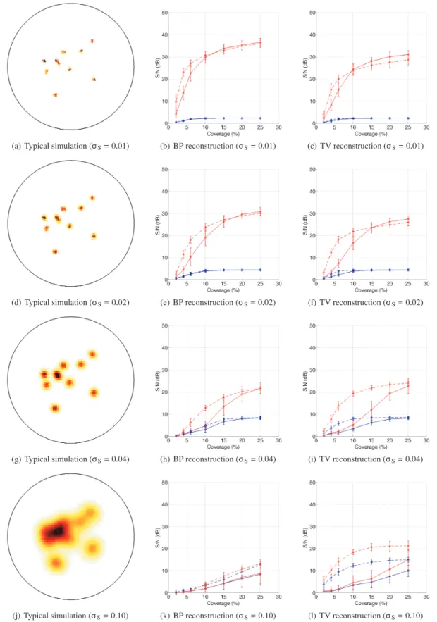
Figure
+5


Documents relatifs