HAL Id: hal-02465656
https://hal.inria.fr/hal-02465656
Submitted on 4 Feb 2020
HAL is a multi-disciplinary open access
archive for the deposit and dissemination of
sci-entific research documents, whether they are
pub-lished or not. The documents may come from
teaching and research institutions in France or
abroad, or from public or private research centers.
L’archive ouverte pluridisciplinaire HAL, est
destinée au dépôt et à la diffusion de documents
scientifiques de niveau recherche, publiés ou non,
émanant des établissements d’enseignement et de
recherche français ou étrangers, des laboratoires
publics ou privés.
Automatic Guided Vehicles: Robust Controller Design
in Image Space
Philippe Martinet, Christian Thibaud
To cite this version:
Philippe Martinet, Christian Thibaud. Automatic Guided Vehicles: Robust Controller Design in
Im-age Space. Autonomous Robots, Springer Verlag, 2000, 8 (1), pp.25-42. �10.1023/A:1008936817917�.
�hal-02465656�
Automatic Guided Vehicles: Robust Controller Design in Image Space
P. MARTINET AND C. THIBAUDLASMEA-GRAVIR, Laboratoire des Sciences et Mat´eriaux pour l’Electronique, et d’Automatique, Universit´e Blaise Pascal de Clermont-Ferrand, U.M.R. 6602 du C.N.R.S., F-63177 Aubi`ere Cedex, France
[email protected] [email protected]
Abstract. We have been interested in Automatic Guided Vehicles (AGV) for several years. In this paper, we synthesize controllers for AGV applications using monocular vision. In particular, we are interested in road following and direction change tasks, and in analyzing the influence of extrinsic camera parameter perturbations on vehicle behavior. We use the bicycle as the kinematic vehicle model, and we choose the position of the white band on the road as the sensor signal. We define an interaction between the camera, which is mounted inside the vehicle, and the white band detected in the image space. Using this kind of interaction, we present how to use a pole assignment technique to solve the servoing task. We show the simulation and experimental results (1/10 scale demonstrator) with and without perturbations. We then investigate the use of a robust controller to slow down the effect of perturbations on the behavior of the vehicle.
Keywords: visual servoing, robust control, mobile robot, vehicles, modeling, vision
1. Introduction
In the realm of intelligent systems for highways, de-velopment of AGV is necessary to enable vehicles to drive automatically along the road (Inrets, 1996; PATH, 1997). In fact, the requirement is for a controller that can maintain the position and the orientation of the vehicle with respect to the center of the road and/or apply changes of direction. The problem of vehicle control using a camera has been given considerable at-tention by many authors (Dickmanns and Zapp, 1987; Kehtarnavaz et al., 1991; Wallace et al., 1986; Waxman et al., 1987). The work described in Jurie et al. (1992, 1993, 1994) is among the most notable in lateral con-trol using monocular vision. It consists of the recon-struction of the road using the 2D visual information extracted from the image processing system (Chapuis et al., 1995).
In recent years, the integration of computer vision in robotics has steadily progressed, from the early “look and move” systems, to current systems in which vi-sual feedback is incorporated directly into the control
loop. These techniques of vision based control are used to control holonomic robots in different domains (Feddema and Mitchell, 1989; Khadraoui et al., 1996; Papanikolopoulos et al., 1991, 1993).
The principle of this approach is based on the task function approach (Samson et al., 1991), and many people have developed this concept applied to vi-sual sensors (Chaumette, 1990; Espiau et al., 1992; Hutchinson et al., 1996). There are still a few appli-cations in mobile robots using this kind of approach. The main difficulty is due to the presence of non-holonomic mechanical connections which limit robot movements (Pissard-Gibollet and Rives, 1991; Tsakiris et al., 1997).
We have proposed a new technique with a visual ser-voing approach, in which control incorporates the vi-sual feedback directly (Khadraoui et al., 1995; Martinet et al., 1997). In other words, this is specified in terms of regulation in the image frame of the camera. Our application involves controlling the lateral road posi-tion of a vehicle following the motorway white line. A complete 2D model of both the vehicle and the scene is
then essential. It takes into account the visual features of the scene and the modeling of the vehicle.
The main purpose of this study is the development of a new lateral control algorithm. We propose a new con-trol model, based on state space representation, where the elements of the state vector are represented by the parameters of the scene, extracted by vision. Then, we use a robust control approach to improve the be-havior of the vehicle when we introduce perturbations in the closed loop to accommodate for mounting inac-curacies, camera calibration errors and driving up an incline.
These approaches were tested with a 1/10 scale demonstrator. It is composed of a cartesian robot with 6 degrees of freedom which emulates the vehicle be-havior and the WINDIS parallel vision system. The road, built to a 1/10 scale, comprises three white lines.
2. Modeling Aspect
Before synthesizing the control laws, it is necessary to obtain models both of the vehicle and of the interaction between the sensor and the environment. We indicate only the main results of modeling aspect presented in Martinet et al., 1997.
2.1. Modeling the Vehicle
It is useful to approximate the kinematics of the steer-ing mechanism by assumsteer-ing that the two front wheels turn slightly differentially. Then, the instantaneous center of rotation can be determined purely by kine-matic means. This amounts to assuming that the steer-ing mechanism is the same as that of a bicycle. Let the angular velocity vector directed along the z axis be called ˙ψ and the linear one directed along the x axis called ˙x.
Orientation equation: Using the bicycle model ap-proximation (see Fig. 1(a)), the steering angleδ and the radius of curvature r are related to the wheel base
L by:
tanδ = L
r (1)
In Fig. 1(b), we show a small portion of a circle1S representing the trajectory to be followed by the vehi-cle. We assume that it moves with small displacements between the initial curvilinear abscissa S0and the final
Figure 1. Bicycle model.
one Sf such that:
1 r = lim1s→0 1ψ 1S = dψ d S = dψ dt dt d S (2)
whereψ represents the orientation of the vehicle. The time derivative of S includes the longitudinal and lateral velocities along the y and x axes respectively. In fact, the rotation rate is obtained as:
˙ψ = tanδ L
p
˙x2+ ˙y2 (3)
Lateral position equation: In order to construct this equation, we treat the translational motion assuming that the vehicle moves with small displacements be-tween t and t+1t. In the case of a uniform movement during a lapse of time1t, the vehicle moves through distance d= V 1t taking V as a constant longitudinal velocity (see Fig. 2).
We express: Sψ = − lim 1t→0 xt+1t − xt V1t = − ˙x V Cψ = ˙y V (4)
Figure 3. Perspective projection of a 3D line.
In these expressions, C and S represent the trigono-metric functions cosine and sine. The approximation to small angles gives us the relation between the differen-tial of the lateral coordinate x and the lateral deviation ψ with respect to δ, expressed as follows:
˙x = −V ψ ˙ψ = V Lδ (5)
2.2. Modeling the Scene
This section shows how to write the equation of the projected line in the image plane, using perspective projection. The scene consists of a 3D line, and its projected image is represented by a 2D line. Figure 3 shows the frames used in order to establish this relation.
We use:
r
Ri = (O, xi, yi, zi) as the frame attached to the 3Dline
r
Rs = (O, xs, ys, zs) as the sensor frame fixed to thecamera
We take into account:
r
h the camera heightr
α the inclination angle of the camerar
ψ the orientation of the vehicleAny 3D point pi = (xi, yi, zi, 1)T related to the
workspace can be represented by its projection in the image frame pp= (xp, yp, zp)T by the relation:
pp = Mpi (6)
The matrix M represents the homogeneous calibra-tion matrix of the camera expressed in the frame Ri.
Its expression is the following:
M = Pc0Cu0CaR2−1R1−1T−1 (7)
where:
r
Pc0Cu0Ca translates ps = (xs, ys, zs)T in pp. Pc0Cu0takes into account the intrinsic parameters of the camera ( fx = f ex, fy = f ey, f the focal length, ex, ey the dimensions of the pixel), and Ca realizes
an exchange coordinates frame.
r
T , R1and R2characterize the extrinsic parameters ofthe camera. T takes into account the two translations of the camera: the height h and the lateral position
x. R1and R2represent the lateral orientationψ and
the inclinationα of the camera respectively. The expressions of the different matrices used are given as follows: Pc0Cu0 = fx 0 0 0 0 fy 0 0 0 0 1 0 , Ca = 1 0 0 0 0 0 −1 0 0 1 0 0 0 0 0 0 T = 1 0 0 x 0 1 0 0 0 0 1 h 0 0 0 1 , R1= Cψ −Sψ 0 0 Sψ Cψ 0 0 0 0 1 0 0 0 0 1 R2= 1 0 0 0 0 Cα −Sα 0 0 Sα Cα 0 0 0 0 1
We note that the second translation and the third rota-tion are considered as null, and that x (lateral posirota-tion) andψ (orientation) are the system variables.
Developing relation 7, we obtain the following ex-pression of M: fxCψ fxSψ 0 fxxCψ − fySαSψ fySαCψ − fyCα − fyx SαSψ + fyhCα −CαSψ CαCψ Sα −xCαSψ + hSα
The pixel coordinates P = (X = xp
zp, Y =
yp
zp)
T
zi = 0), are expressed by: X = fx yiSψ + xCψ yiCαCψ − xCαSψ + hSα Y = fy−yiSαCψ − x SαSψ + hCα yiCαCψ − xCαSψ + hSα (8)
Eliminating yi from the Eqs. (8), we obtain:
X = fx fy · xCα − hSψ Sα hCψ ¸ Y + fx · x Sα + hSψCα hCψ ¸ (9) Considering thatα and ψ are small (<10 deg) and if we neglect the product termαψ, the second order Taylor approximation gives us a new expression of X :
X= fxx fyh Y+ fx µ xα h + ψ ¶ + O(ψ2) + O(α2) (10)
The equation of the line expressed in the image frame is given by the following relation:
X = aY + b (11)
where(a, b) are the line parameters expressed by:
a = fxx fyh = µ1x b= fx µαx h + ψ ¶ = µ2x+ µ3ψ (12)
We express the lateral position x and the orientation of the vehicleψ in order to define an interaction rela-tion between the 3D posirela-tion of the vehicle and the 2D parameters of the line in the image plane. We have:
˙x = h fy fx ˙a = ξ1˙a ˙ψ = −αfy fx ˙a + 1 fx˙b = ξ 2˙a + ξ3˙b (13)
with: fx= 1300 pu, fy= 1911 pu, V = 20 km/h, L =
0.3 m and h = 0.12 m (in our 1/10 scale demonstrator).
3. Pole Assignment Approach
In this section, we present the application of the pole as-signment technique when the state model is expressed
directly in the sensor space. In our case, the sensor space is the image plane.
The controller design is based on the kinematic model of the vehicle. We use the(a, b) parameters of the 2D line in the image plane as the state vector. We steer the vehicle by acting on wheel angleδ. We choose b or a as the output parameter of the system and use the results of the vehicle and scene modelings to obtain the following equation:
(
−V ψ = ξ1˙a
(V/L)δ = ξ2˙a + ξ3˙b
(14)
The state vector, denoted by X = (a, b)T, is equal
to the sensor signal vector in the state space represen-tation. Developing, we have the following state model of the system:
(
˙X = AX + BU
y= C X (15)
with U = δ the wheel angle, y the output of the system, and A= − Vξ2 ξ1 − Vξ3 ξ1 Vξ2 2 ξ1ξ3 Vξ2 ξ1 , B = " 0 V Lξ3 # C= [0, 1] or = [1, 0]
depending on the output to be controlled. The visual servoing scheme is then as shown in Fig. 4.
Finally, we can express the control law by the fol-lowing relation:
U = δ = −k1a− k2b+ ky∗ (16)
where K = [k1, k2] and k are the gains of the control
law obtained by identifying the system to a second or-der system characterized byω0 andξ. y∗ represents
the input of the control scheme.
For the first step, we chose parameter b as the out-put of the system and analysed the effects of pertur-bation. For the second, we replaced parameter b by parameter a.
3.1. Choice of b as the Output of the System
3.1.1. Controller Design. Here, we present the
ap-plication of the pole assignment technique when the state model is expressed directly in the sensor space. We choose b as the output parameter of the system. So, we can write:
(
˙X = AX + Bδ
b= C X (17)
and, we can express the control law by the following relation:
δ = −k1a− k2b+ kb∗ (18) where K = [k1, k2] and k are the gains of the control
law obtained by identifying the system to a second or-der system characterized byω0andξ. For these control
gains, we obtain: k1= Lω0(2ξ2ξ V − ξ1ω0) V2 k2= 2Lω0ξ3ξ V k = Lω 2 0ξ1ξ3 V2ξ 2 (19)
We note that, as expressed by these relations, the higher the velocity V , the smaller are the gains.
3.1.2. Simulation and Experimental Results. To
val-idate this control law, we use a simulator developed with Matlab. Figure 5 shows the visual servoing scheme used in this simulator.
We use the kinematic model of the vehicle to simu-late the behavior of the vehicle, and the perspective
Figure 5. Visual servoing scheme of the simulator.
Figure 6. b without perturbations (α = −7 degrees) (simulation results).
projection relation to obtain the sensor signal s = (a, b)T. The first results (see Fig. 6) illustrate the
out-put behavior of the system corresponding to an inout-put value b∗= 100 pixels. We take into account a data flow latency (three sample periods) in all simulation tests. This was identified on our experimental site. We chose ω0 = 2rd/s and ξ = 0.9 in order to fix the behavior
of the system. In this case, we have no perturbations (α is fixed at −7 degrees).
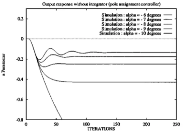
The second set of results takes into account a per-turbed angleα (from −6 to −10 degrees). We obtain the following response in b: Fig. 7 represents the simu-lation results, and Fig. 8 shows the experimental results obtained with our 1/10 scale demonstrator presented in Section 6.
In both results, we can see a steady state error in b, when we introduce the perturbations, and some oscil-lations appear when angleα increases. In this case, ξ slows down from 0.9 (α = −7) to 0.6 (α = −10) and increases the overtaking, but the main contribution to
Figure 8. b output behavior (experimental results).
the oscillations is due to the data flow latency. In the next section, we express the steady state error in order to analyze the simulation and experimental results.
3.1.3. Closed Loop Steady State Error Estimation.
Here we analyse the behavior of the vehicle when the extrinsic parameters of the camera are perturbed. In this case, Eqs. (13) show us that only ξ1 andξ2 are
affected by perturbations of this kind.
Considering the state Eqs. (17) and taking into ac-count parameter perturbations, we have:
A= − V(ξ2+1ξ2) ξ1+1ξ1 − Vξ3 ξ1+1ξ1 V(ξ2+1ξ2)2 (ξ1+1ξ1)ξ3 V(ξ2+1ξ2) ξ1+1ξ1
Figure 9 represents the general visual servoing scheme, using the pole assignment approach.
In this case, we can establish the general expression of the steady state error ²∞ by using the Laplace p transform by:
²(p) = b∗(p) − b(p) (20)
with:
b(p) = C[pI − (A − BK )]−1Bkb∗(p) (21)
Figure 9. Steady state error.
Table 1. Steady state error²∞.
α in degrees ²∞measured ²∞computed
−8 35 37
−9 49 56
−10 55 62
Hence we obtain:
²∞= [1 + C(A − BK )−1Bk] b∞∗ (22) After some developments and approximations, we can write the final relation of the steady state error as follows: ²∞= " 1− 1+ 1ξ2 ξ2 1+2Vξξ2 ω0ξ1 1ξ2 ξ2 # b∗∞ (23)
The steady state error becomes null, if the following expression is true:
1ξ2
ξ2
=1α
α = 0 (24)
We observe that, in the absence of perturbations in theα parameter, we have no steady state error. When α is different from the reference value, we obtain an error which confirms all the simulation results.
In this experiment, we can verify the values of steady state error for different values of theα parameter (see Table 1).
The difference between reference and experimental values can be explained by the imprecise calibration of the interaction between the scene and the camera.
In the next section, we show the way to reduce this steady state error.
3.1.4. Pole Assignment with Integrator. In this sec-tion, we introduce an integrator into the control law in order to eliminate the steady state error in case of per-turbations. The visual servoing scheme is represented in Fig. 10.
In this case, we can express the control law by the relation:
δ = −k1a− k2b− Ki Z
(b∗− b) dt (25)
where k1, k2and Kiare the gains of the control law
ob-tained by identifying the system to a third order system characterized by the following characteristic equation: (p2+ 2ξω
0p+ ω20)(p + ξω0). The control law gains
are given by:
k1 = − Lω0(2ω0ξ1ξ2− 3ξ2ξ V + ω0ξ1) V2 +Lω30ξ 2 1ξ V3ξ 2 k2 = 3Lω0ξ3ξ V Ki = − Lω03ξ1ξ3ξ V2ξ 2 (26)
In the first simulation, we consider no perturbations. Figure 11 illustrates the fact that the response time is correct.
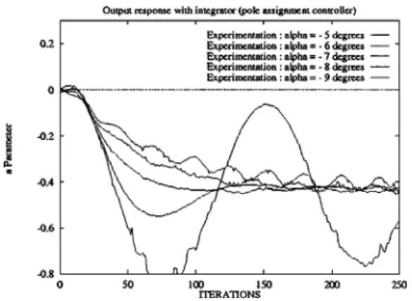
Secondly, we introduce some perturbations in theα angle (from−6 to −10 degrees). Figure 12 shows the simulation results and Fig. 13 shows the experimental ones.
In fact, no steady state error persists during servoing, but some oscillations and problems of stability appear whenα is very different from the reference value.
We therefore decided to analyse the same approach using the other parameter.
Figure 11. b without perturbations (α = −7) (simulation results).
Figure 12. b output behavior (simulation results).
Figure 13. b output behavior (experimental results). 3.2. Choice of a as the Output of the System
In this part, we choose a as the output parameter of the system. We can then write:
(
˙X = AX + Bδ
a = C X (27)
and we can express the control law by the following relation:
δ = −k1a− k2b+ ka∗ (28)
where K = [k1, k2] and k are the gains of the control
law, expressed by the following relations:
k1 = Lω0(2V ξ2ξ − ω0ξ1) V2 k2 = 2Lω0ξ3ξ V k = −Lω 2 0ξ1 V2 (29)
Figure 14. a with perturbations (α = −6 to −10) (simulation results).
Figure 15. a with perturbations (α = −6 to −10) (experimental results).
We note that, as we observed with parameter b, the higher the velocity V , the smaller are the gains.
We tested this approach as we did for parameter b. When no static perturbations occurred, the output behavior corresponds to the desired output (a∗= 0.43) in both simulation (Fig. 14) and experimental (Fig. 15 ) cases. If we introduce this kind of perturbation into the α parameter, steady state error and oscillations appear on the output of the system.
As before, we can express the steady state error in the following form:
²∞= [1 + C(A − BK)−1Bk] a∗∞ (30) and after some developments, we obtain:
²∞= " 1− 1 1+2Vξξ2 ω0ξ1 1ξ2 ξ2 # a∞∗ (31)
The steady state error becomes null, if the following expression is verified:
1ξ2
ξ2
=1α
α = 0 (32)
We observe that, in the absence of perturbations to theα parameter, we have no steady state error.
We therefore introduce an integrator into the control law in order to eliminate this steady state error in case of perturbations.
The control law is expressed by the relation: δ = −k1a− k2b− Ki
Z
(a∗− a) dt (33)
where k1, k2and Ki are the gains of the control law: k1 = 3Lω0ξ2ξ V − Lω2 0ξ1 V2 (2ξ 2+ 1) k2 = 3Lω0ξ3ξ V Ki = Lω03ξξ1 V2 (34)
We tested the output behavior of the system in the presence of perturbations toα angle (from −5 to −9 degrees). Figure 16 illustrates the simulation results and Fig. 17 the experimental ones.
As we can see, no steady state error persists during servoing, but some oscillations and problems of stabil-ity appear whenα is far from the reference value. These results are close to those encountered when using pa-rameter b. We therefore conducted investigations into robust control approaches, particularly into H∞space control.
Figure 16. a with perturbations (α = −5 to −9) (simulation results).
Figure 17. a with perturbations (α = −5 to −9) (experimental results).
4. Robust Control Approach
Due to the the problem of oscillations and stability encountered when using a pole assignment approach, we decide to investigate a robust control approach. We chose the approach developed in H∞space at the begin-ning of the eighties (Zames and Francis, 1983; Kimura, 1984; Dorato and Li, 1986; Doyle et al., 1989), concerning controller design with plant uncertainty modeled as unstructured additive perturbations in the frequency domain.
4.1. Generality Concerning H∞Space
Here, we present the application of the robust con-trol technique, particularly in H∞space (Dorato et al., 1992).
The servoing scheme is presented in the Fig. 18. We consider an additive perturbation in the fre-quency domain:
F(p) = F0(p) + 1F0(p) (35)
where F0(p) represents the nominal transfer function.
Figure 18. Servoing scheme in H∞space.
The aim is to determine a single robust controller
c(p) which ensures the stability of the closed loop
sys-tem. Then, we can write 1+ F(p) · c(p) as:
[1+ F0(p) · c(p)] · · 1+ c(p) 1+ F0(p) · c(p) · 1F0(p) ¸ = [1 + F0(p) · (p)] · [1 + q(p) · 1F0(p)] (36) with q(p) =1+Fc(p) 0(p)·c(p).
To ensure the stability of the close loop system, we must verify:
|1 + F( jω) · c( jω)| 6= 0 ∀ω (37) We define a transfer function r( jω) which bounds the variations of F0( jω) as:
|1F0( jω)| ≤ |r( jω)| |r( jω)| F0( jω) ≤ 1 ∀ω (38)
In this case, if c(p) stabilizes the nominal plant
F0(p) we can express the robust stability condition as
(Kimura, 1984):
kq(p)r(p)k∞< 1 (39)
In these conditions, the robust controller can be ex-pressed by:
c(p) = q(p)
1− F0(p)q(p)
(40)
General Case. In this part we summarize the differ-ent steps to follow to synthesize a robust controller. The function r(p) bounds the variations of F0(p). We
construct the proper stable function:
e
F0(p) = B(p) · F0(p) (41)
where B(p) =Q(pi−p
¯pi+p) represents the Blaschke
prod-uct of unstable poles pi (Re(pi) > 0) of F0(p).
For convenience, we defineeq(p) as:
q(p) = B(p) · eq(p) (42) and then:
We have to choose a minimal phase function rm(p)
as:
|rm( jω)| = |r( jω)| (44) In this case, we can express r(p) = b(p) · rm(p),
where b(p) is an inner function (|b( jω)| = 1, ∀ω). The robust condition of stability can be rewritten as:
ku(p)k∞< 1 with u(p) = eq(p) · rm(p) (45)
Using relation 43, and since the function 1− F0(p) · q(p) has the zeros at the unstable poles αi of F0(p),
we can express the first interpolation conditions with:
eq(αi) =
1
e F0(αi)
∀i = 1, . . . , l (46) Sinceeq(p) and rm(p) are H∞functions, the
func-tion u(p) must be an SBR function (Strongly Bounded Real), and the conditions of interpolation can be written as: u(αi) = eq(αi) · rm(αi) = rm(αi) e F0(αi) = βi (47)
(βi represents an interpolation point). So the solution
to the problem of robust stabilization of an unstable system (Kimura, 1984) lies in finding an SBR function
u(p) which interpolates to the points u(αi). This
lem is called the Nevanlinna-Pick interpolation prob-lem. Dorato et al. in (Dorato and Li, 1986) have pro-posed an iterative solution of this problem based on the interpolation theory of Youla and Saito (Youla and Saito, 1967). When the relative degree of the function
rm(p) is greater than 0, we must append one or more
supplementary interpolation conditions near infinity.
Case of a Plant With Two Poles at the Origin.
Pre-vious work (Kimura, 1984; Dorato et al., 1992; Byrne and Chaouki, 1994; Byrne et al., 1997) has shown how to consider the case of a plant with integrators. We can define:
r(p) = r
0
m(p)
p2 (48)
where rm0(p) is a minimal phase function and:
e
F0(p) = p2· B(p) · F0(p) eq(p) = q(p)
p2· B(p)
(49)
Using relation 43, we can write the following con-ditions of interpolation: eq(αi) = 1 e F0(αi) ∀i = 1, . . . , l eq(0) = 1 e
F0(0) 2 poles at the origin
(50)
To ensure that c(p) is a robust controller, the func-tion u(p) = rm0(p) · eq(p) must be an SBR function
which satisfies the interpolation conditions at the un-stable poles of the function F0(p) and also at the origin
with the relations:
u(αi) = rm0(αi) e F0(αi) ∀i = 1, . . . , l u(0) = r 0 m(0) e F0(0)
2 poles at the origin
(51)
In these conditions, the function q(p) can be ex-pressed by:
q(p) = p
2· B(p) · u(p)
rm0 (p) (52)
4.2. Controller Design Using Parameter b
Previous results have been presented in (Martinet et al., 1998a, b).
Considering parameter b as the output of the system, we define: F1(p) = b δ = V2ξ2+ pξ1V ξ1p2Lξ3 1F1(p) F1(p) = |1α α | + |1hh | 1+ ξ1 V·ξ2· p (53)
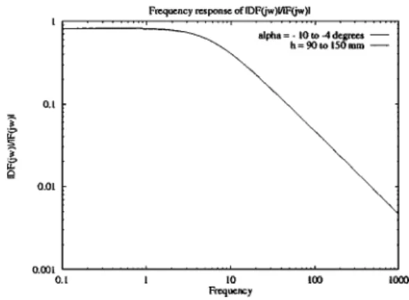
Using the following expression of r(p):
r(p) = sup ω ¯¯ ¯¯1F1( jω) F1( jω) ¯¯ ¯¯F1(p) (54)
and looking at Fig. 19, we can consider rm0(p) as:
rm0(p) = K1· p2· F1(p) with K1= 0.82 (55)
To determine the value of K1, we have to plot the
quantity|1F1( jω)
F1( jω)| considering the following perturba-tions:
1α
α = 57% and
1h
Figure 19. Frequency response of|1F1( jω)
F1( jω)|.
Since F1(p) has no unstable pole, the function B(p) = 1, and we have to choose u(p) as an SBR
function with a relative degree of 1 (because of the expression of rm0(p)).
We choose the following expression of u(p):
u(p) = K1
1+ τ · p (56)
to satisfy the conditions of interpolation:
u(0) = r 0 m(0) e F1(0) = K1at the origin u(∞) = 0 (57)
We deduce the expression of the function q(p):
q(p) = p 2· K 1 (1 + τ · p) · K1· p2· F1(p) = (ξ1p2Lξ3) (1 + τ · p) · (V2ξ 2+ pξ1V) (58) and developing, we obtain the robust controller c(p):
c(p) = 1 τ · p · F1(p) = ξ1pLξ3 τ · (V2ξ 2+ pξ1V) (59)
4.3. Controller Design Using Parameter a
Considering parameter a as the output of the system, we define: F2(p) =a δ = − V2 ξ1Lp2 1F2(p) F2(p) = ¯¯ ¯¯1hh ¯¯¯¯ (60)
As previously, we use the following expression of
r(p): r(p) = sup ω ¯¯ ¯¯1F2( jω) F2( jω) ¯¯ ¯¯F2(p) (61)
and looking at the expression of F2(p), we can consider rm0(p) as:
rm0(p) = K2· p2· F2(p) with K2= 0.25 (62)
Since F2(p) has no unstable pole, we have to choose u(p) as an SBR function with a relative degree of 2
(because of the expression of rm0(p)).
We choose the following expression of u(p):
u(p) = K2
(1 + τ · p)2 (63)
and the conditions of interpolation are the following:
u(0) = r 0 m(0) e F2(0)= K2at the origin u(∞) = 0 (64)
We deduce the expression of the function q(p):
q(p) = p 2· K 2 (1 + τ · p)2· K 2· p2· F2(p) = − ξ1L p2 (1 + τ · p)2· V2 (65)
and developing, we obtain the robust controller c(p):
c(p) = 1
τ · p · (2 + τ · p) · F2(p)
= − ξ1L p
τ · (2 + τ · p) · V2 (66) 4.4. Simulation and Experimental Results
As for the pole assignment technique, we have de-veloped a simulator in matlab. We introduce pertur-bations to angleα (from α = −3 to α = −11) during simulation.
Figures 20 and 21 show the simulation and experi-mental results of a robust control approach using b pa-rameter as the output of the system(b∗ = 100 pixels). In these experiments we chooseτ = 0.67. There is no
Figure 20. b output behavior (α from −3 to −11 degrees) (simu-lation results).
Figure 21. b output behavior (α from −3 to −11 degrees) (experi-mental results).
steady state error during servoing and the robustness is much improved.
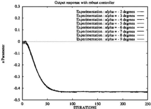
As a second step, we use the parameter a of the line as the output of the system, to synthesize a new robust controller using the H∞ technique. In these experiments we chooseτ = 0.5.
The simulation and experimental results are pre-sented in Figs. 22 and 23. The output behavior of the system corresponding to a reference input value
a∗ = 0.43 is illustrated. As we can see, there is no
steady state error in the output response and the output behavior remains unchanged when we introduce per-turbations to α angle. So we can conclude that both theorical and experimental results tend to select para-meter a as the output of the system.
In the next section, we discuss 3D lateral position behavior during servoing and we analyze the effect of camera height perturbation when using the previous robust controller.
Figure 22. a output behavior (α from −2 to −9 degrees) (simula-tion results).
Figure 23. a output behavior (α from −2 to −9 degrees) (experi-mental results).
5. Discussion
As we have seen in the previous section, it is better to choose parameter a of the 2D line as the output of the system. So, in the following we develop only the discussion concerning this choice. We first analyse the lateral position behavior of the vehicle and the effect of camera height perturbation. We conclude the dis-cussion by considering the coupling of perturbations.
5.1. Lateral Position Behavior
In this part, we present the lateral position behavior of the vehicle (simulated on our 1/10 scale demonstrator). We present successively the results of:
r
pole assignment with integrator (Fig. 24)Figure 24. Lateral position behavior (pole assignment) (experi-mental results).
Figure 25. Lateral position behavior (robust control) (experimental results).
when using the a parameter of the 2D line as the output of the system.
If we look at these figures, we can compare the be-havior of the lateral position of the vehicle. When using the pole assignment technique, the lateral position of the vehicle is sensitive to perturbations. Oscillations and divergence occur when angleα is far from the ref-erence value. On the other hand, the robust controller is very efficient and the robustness is greatly improved. We think that the weak variations of the lateral posi-tion observed on the curves may have been produced by small perturbations to camera height (see Eq. (12)) dur-ing the experiments (imprecise calibration). We con-clude that behavior is more efficient and stable when using a robust controller.
5.2. Camera Height Perturbation
To clarify and analyze the sensitivity of the control laws on perturbations, we decided to study the effect of camera height perturbation.
Figure 26. Perturbation of camera height.
Figure 27. Lateral position behavior (experimental results).
We fixed the variations of camera height at 25% of the reference value (0.12 m) (Fig. 26).
Figure 27 presents the lateral position behavior when using both approaches.
We observe a lateral deviation of the vehicle in both approaches. We can verify these results by looking at relation 12, where the lateral position of the vehicle
x is directly linked to parameter a through the
cam-era height parameter. Even if in both cases a latcam-eral deviation is present, the robust controller is smoother and induces better behavior of the linkage between the vision aspect and the control aspect.
As in a real scene, it is unrealistic to think that pertur-bations will occur separately. So we decided to study the effect of coupled perturbations.
5.3. Coupling Perturbations
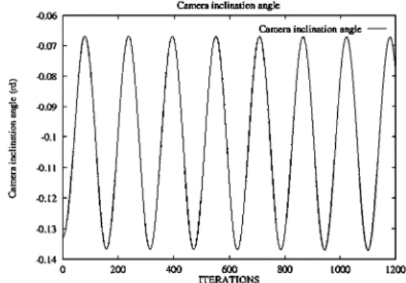
In the first test, we introduced perturbations into camera height (25%) (Fig. 28) and camera inclination angle (±1 and ±2 degrees) (Fig. 29).
Figure 28. Perturbation on camera height.
Figure 29. Perturbation to camera inclination angle.
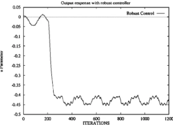
Figure 30. Parameter a (robust and pole assignment control) (ex-perimental results).
Using the parameter a as the output of the system, we compared the pole assignment and robust control ap-proaches. Figure 30 shows the output behavior of the system (a parameter) and Fig. 31 presents the lateral position behavior of the vehicle. As shown previously,
Figure 31. Lateral position behavior (robust and pole assignment control) (experimental results).
Figure 32. Perturbation on camera roll angle.
robust control minimizes the effect of camera inclina-tion angle perturbainclina-tion, but even if the other pertur-bation is also minimized, the effect on the 3D lateral position remains considerable.
With these results, we definitively conclude that the robust control approach is better than the pole assign-ment approach.
In the second test, we append perturbation on camera roll angle (sinusoid of±2 degrees) (Fig. 32).
Figure 33 presents the evolution of the output system. As we can see the robust controller is more efficient, and we observe also that the effect on lateral position behavior is better when using this kind of controller (see Fig. 34). But the simplified model is not sufficient to take all of these perturbations into account.
In the third test, we use sinusoid functions to inject perturbation into extrinsic camera parameters:
Figure 33. Parameter a (robust and pole assignment control) (ex-perimental results).
Figure 34. Lateral position behavior (robust and pole assignment control) (experimental results).
r
camera inclination angle (sinusoid of ±1 degree) (Fig. 36),r
camera height (sinusoid of±10 mm ) (Fig. 37). Figure 38 presents the lateral position behavior of the vehicle and Fig. 39 the output behavior of the system. Even if the effect of the roll angle perturbation is at-tenuated, there is an offset which appears on the output of the system and on the lateral position of the vehicle. As regards these tests, we conclude that these ap-proaches are subject to two limitations. The model of the interaction between the sensor and the scene does not take roll angle into account, and there is a problem in the presence of camera height perturbation. 6. The Path to ImplementationUntil now, we have not had a real demonstrator. So, these approaches were tested with a 1/10 scale demonstrator. It is composed of a cartesian robot with
Figure 35. Perturbation to camera roll angle.
Figure 36. Perturbation on camera inclination angle.
Figure 37. Perturbation on camera height.
6 degrees of freedom (built by the firm AFMA Robot) and the WINDIS parallel vision system (Martinet et al., 1991; Rives et al., 1993).
This whole platform (see Fig. 40) is controlled by a VME system, and can be programmed in C language under the V×Works real time operating system. The CCD camera is embedded on the end effector of the
Figure 38. Lateral position behavior (robust control) (experimental results).
Figure 39. Parameter a (robust control) (experimental results).
Figure 40. Overview of the experimental site.
cartesian robot and is connected to the WINDIS vision system. In this servoing scheme the position of the dif-ferent parts of the controller changes with the approach under consideration.
The road (see Fig. 41), built to a 1/10 scale, com-prises three white lines. For each level of this vision system, we have introduced parallelism allowing us to reach video rate for most of the application tasks. The vision system computes the (a, b) parameters of the
Figure 41. 1/10 scale road.
projected line in the image plane at video rate (25 Hz). In this implementation, we have identified a data flow latency of three sample periods.
Now, we are working on the conception of a real demonstrator with the lateral and longitudinal control capabilities. We think that the main difficulties to path to real implementation should be the continuous extrac-tion of visual informaextrac-tions in real environment, and the effectivness of the approaches described above.
7. Conclusion and Future Work
Controllers based on a visual servoing approach have been developed in this paper. We designed a controller with a pole assignment technique directly in the im-age space. After modeling the vehicle and the scene, we obtained equations which can be used to write the state model of the system. Visual servoing is performed well when there are no perturbations. When perturba-tions occur, a steady state error and oscillaperturba-tions appear. By introducing an integrator into the visual servoing scheme, we suppress the steady state error but amplify the oscillation problem.
We then investigated a robust control approach. The choice of b as the output parameter of the system does not permit the control of the lateral position of the vehicle precisely when the perturbations appear, but ensures control of heading. The choice of parameter
a as the output of the system, to synthesize a new
ro-bust controller, seems to be sufficient when we have perturbations toα angle and camera height.
In the future, we will investigate a controller which can take into account a combination of perturbations to α angle, camera height and camera roll angle. For this purpose, we shall require improved models both of the scene and of the vehicle. The robust control approach is well adapted in this case, because this approach is efficient when we use more complex models. So an
extension of this work using dynamic modeling can be considered.
We think that experimentation on a real vehicle will be necessary to validate all of the results presented in this paper.
References
Byrne, R.H. and Chaouki, A. 1994. Robust lateral control of highway vehicles. In Proceedings of Intelligent Vehicle Symposium, Paris, France, pp. 375–380.
Byrne, R.H., Chaouki, A., and Dorato, P. 1997. Experimental re-sults in robust lateral control of highway vehicles. IEEE Control Systems, pp. 70–76.
Chapuis, R., Potelle, A., Brame, J.L., and Chausse, F. 1995. Real-time vehicle trajectory supervision on the highway. The Interna-tional Journal of Robotics Research, 14(6):531–542.
Chaumette, F. 1990. La relation vision commande: th´eorie et ap-plication `a des tˆaches robotiques. Ph.D. Thesis, IRISA/INRIA, Rennes, France.
Dickmanns, E.D. and Zapp, A. 1987. Autonomous high speed road vehicle guidance by computer. In Proceedings of 10th IFAC World Congress.
Dorato, P., Fortuna, L., and Muscato, G. 1992. Robust Control for Un-structured Perturbations—An Introduction, Springer-Verlag, Lec-tures Notes in Control and Information Sciences, Vol. 168. Dorato, P. and Li, Y. 1986. A modification of the classical
nevanlinna-pick interpolation algorithm with applications to robust stabiliza-tion. IEEE Transactions on Automatic Control, 31(7):645–648. Doyle, J., Glover, K., Khargonekar, P., and Francis, B. 1989. State
space solutions to standard H2and H∞control problems. IEEE
Transactions on Automatic Control, 34(8).
Espiau, B., Chaumette, F., and Rives, P. 1992. A new approach to visual servoing in robotics. IEEE Transactions on Robotics and Automation, 8(3):313–326.
Feddema, J.T. and Mitchell, O.R. 1989. Vision-guided servoing with feature-based trajectory generation. IEEE Transactions on Robotics and Automation, 5(5):691–700.
Hutchinson, S., Hager, G.D., and Corke, P. 1996. A tutorial on visual servo control. IEEE Transactions on Robotics and Automation, 12(5):651–670.
Inrets. 1996. La route automatis´ee-r´eflexions sur un mode transport futur. Technical Report, INRETS.
Jurie, F., Rives, P., Gallice, J., and Brame, J.L. 1992. A vision based control approach to high speed automatic vehicle guidance. In Proceedings of IARP Workshop on Machine Vision Applications, Tokyo, Japan, pp. 329–333.
Jurie, F., Rives, P., Gallice, J., and Brame, J.L. 1993. High speed automatic vehicle guidance based on vision. In Proceedings of Intelligent Autonomous Vehicle, Southampton, United Kingdom, pp. 205–210.
Jurie, F., Rives, P., Gallice, J., and Brame, J.L. 1994. High-speed vehicle guidance based on vision. Control Engineering Practice, 2(2):287–297.
Kehtarnavaz, N., Grisworld, N.C., and Lee, J.S. 1991. Visual control for an autonoumous vehicle (BART)-the vehicle following prob-lem. IEEE Transactions on Vehicular Technology, 40(3):654–662.
Khadraoui, D., Martinet, P., and Gallice, J. 1995. Linear control of high speed vehicle in image space. In Proceedings of Second In-ternational Conference on Industrial Automation, Nancy, France IAIA, Vol. 2, pp. 517–522.
Khadraoui, D., Motyl, G., Martinet, P., Gallice, J., and Chaumette, F. 1996. Visual servoing in robotics scheme using a camera/laser-stripe sensor. IEEE Transactions on Robotics and Automation, 12(5):743–749.
Kimura, H. 1984. Robust stabilization for a class of transfer fonction. IEEE Transactions on Automatic Control, 29:788–793. Martinet, P., Khadraoui, D., Thibaud, C., and Gallice, J. 1997.
Controller synthesis applied to automatic guided vehicle. In Pro-ceedings of Fifh Symposium on Robot Control, SYROCO, Nantes, France, Vol. 3, pp. 735–742.
Martinet, P., Rives, P., Fickinger, P., and Borrelly, J.J. 1991. Parallel architecture for visual servoing applications. In Proceedings of the Workshop on Computer Architecture for Machine Perception, Paris, France, pp. 407–418.
Martinet, P., Thibaud, C., Khadraoui, D., and Gallice, J. 1998a. First results using robust controller synthesis in automatic guided vehicles applications. In Proceedings of Third IFAC Symposium on Intelligent Autonomous Vehicles, IAV, Madrid, Spain, Vol. 1, pp. 204–209.
Martinet, P., Thibaud, C., Thuilot, B., and Gallice, J. 1998b. Robust controller synthesis in automatic guided vehicles applications. In Proceedings of the International Conference on Advances in Vehi-cle Control and Safety, AVCS’98, Amiens, France, pp. 395–401. Papanikolopoulos, N., Khosla, P.K., and Kanade, T. 1991. Vision and control techniques for robotic visual tracking. In Proceedings of the IEEE International Conference on Robotics and Automation, Sacramento, USA.
Papanikolopoulos, N., Khosla, P.K., and Kanade, T. 1993. Visual tracking of a moving target by a camera mounted on a robot: A combination of control and vision. IEEE Transactions on Robotics and Automation, 9(1):14–35.
PATH. 1997. California path–1997 annual report. Technical Report, PATH.
Pissard-Gibollet, R. and Rives, P. 1991. Asservissement visuel ap-pliqu´e `a un robot mobile: ´Etat de l’art et mod´elisation cin´ematique. Technical Report 1577, Rapport de recherche INRIA.
Rives, P., Borrelly, J.L., Gallice, J., and Martinet, P. 1993. A versa-tile parallel architecture for visual servoing applications. In Pro-ceedings of the Workshop on Computer Architecture for Machine Perception, News Orleans, USA, pp. 400–409.
Samson, C., Borgne, M. Le, and Espiau, B. 1991. Robot Control: The task function approach. Oxford University Press. ISBN 0-19-8538057.
Tsakiris, D.P., Rives, P., and Samson, C. 1997. Applying visual ser-voing techniques to control nonholonomic mobile robot. In Pro-ceedings of the Workshop on New trends in Image-Based Robot Servoing, IROS’97, Grenoble, France, pp. 21–32.
Wallace, R., Matsuzak, K., Goto, Y., Crisman, J., Webb, J., and Kanade, T. 1986. Progress in robot road following. In Proceedings of the IEEE International Conference on Robotics and Automa-tion.
Waxman, A.M., LeMoigne, J., Davis, L.S., Srinivasan, B., Kushner, T.R., Liang, E., and Siddalingaiah, T. 1987. A visual naviga-tion system for autonomous land vehicles. IEEE Transacnaviga-tions on Robotics and Automation, 3(2):124–141.
Youla, D.C. and Saito, M. 1967. Interpolation with positive-real func-tions. J. Franklin Inst., 284(2):77–108.
Zames, G. and Francis, B.R. 1983. Feedback, minimax sensitivity, and optimal robustness. IEEE Transactions on Automatic Control, AC-28(5):585–601.
Philippe Martinet was born in Clermont-Ferrand, France 1962. He received his Electrical Engineering Diploma from the CUST, University of Clermont-Ferrand, France, in 1985, and the Ph.D. degree in Electrical Engineering from the Blaise Pascal University of Clermont-Ferrand, France, in 1987. He spent three years in the Electrical industry. Since 1990, he has been assistant professor of Computer Science at the CUST, Blaise Pascal University of Clermont-Ferrand, France. His research interests include visual
servoing, vision based control, robust control, Automatic Guided Vehicles, active vision, visual tracking, and parallel architecture for visual servoing applications. He works in the LASMEA Laboratory, Blaise Pascal University, Clermont-Ferrand, France.
Christian Thibaud was born near Clermont-Ferrand, France 1944. He received the Ph.D. degree and the Doctorat d’Etat `es Science from the Blaise Pascal University of Clermont-Ferrand, France, respectively in 1971 and 1981. Since 1988, he has been profes-sor of Computer Science at the CUST, Blaise Pascal University of Clermont-Ferrand, France. His research interests include visual ser-voing, robust control, Automatic Guided Vehicles. He works in the LASMEA Laboratory, Blaise Pascal University, Clermont-Ferrand, France.