Tracking 3D Object using Flexible Models

HAL Id: inria-00548508

https://hal.inria.fr/inria-00548508

Submitted on 20 Dec 2010

HAL is a multi-disciplinary open access

archive for the deposit and dissemination of

sci-entific research documents, whether they are

pub-lished or not. The documents may come from

teaching and research institutions in France or

abroad, or from public or private research centers.

L’archive ouverte pluridisciplinaire HAL, est

destinée au dépôt et à la diffusion de documents

scientifiques de niveau recherche, publiés ou non,

émanant des établissements d’enseignement et de

recherche français ou étrangers, des laboratoires

publics ou privés.

Tracking 3D Object using Flexible Models

Lucie Masson, Michel Dhome, Frédéric Jurie

To cite this version:

Lucie Masson, Michel Dhome, Frédéric Jurie. Tracking 3D Object using Flexible Models. British

Machine Vision Conference (BMVC ’05), Sep 2005, Oxford, United Kingdom. �inria-00548508�

Tracking 3D Objects using Flexible Models

Lucie Masson

Michel Dhome

Fr´ed´eric Jurie

_{LASMEA - CNRS UMR 6602 - Universit´e Blaise-Pascal,}

2

_{GRAVIR - CNRS UMR 5527 - INRIA Rhone-Alpes - INPG - UJF,}

masson,dhome@lasmea.univ-bpclermont.fr, frederic.jurie@inrialpes.fr

Abstract

This article proposes a flexible tracker which can estimate motions and de-formations of 3D objects in images by considering their appearances as non-rigid surfaces. In this approach, a flexible model is built by matching local features (key-points) over training sequences and by learning the deforma-tions of a spline based model. A statistical model captures the variadeforma-tions of object appearance caused by 3D pose variations. Visual tracking is then pos-sible, for each new frame, by matching the local features of the model with the image features, according to their local appearances and the constraints provided by the flexible model. This approach is demonstrated on real-world image sequences.

1

Introduction

Visual tracking and more generally analysis of image sequences is one of the basic tasks usually involved in computer vision applications. The scope of these potential applica-tions is very wide, including estimation of camera motion, image registration, video com-pression, video surveillance or extraction of 3D scene features. The common problem can often be summarized as establishing correspondences between consecutive frames of an image sequence.

Visual tracking has been addressed by different frameworks. Algorithms based on the matching of local information or features [4, 10, 14] are often distinguished from those considering objects as regions of the image, taken as a whole [2, 5, 7].

The proposed approach belongs to the first category, as it is based on the matching of local features over an image sequence. The key difference with standard feature-based tracking methods is that we represent 3D object appearances using deformations of smoothed 2D ’TPS’ splines. Splines impose a natural smoothness constraint on the feature motion and give the flexibility needed to represent 3D pose variations, seen as 2D image deformations.

In our approach, relations between 2D spline deformations and 3D pose variations are learned offline during a training stage. This stage consists in collecting a set of images representing the possible appearances of an object captured from different view-points. The central view point is called the ’frontal key view’. A feature based matching process

automatically registers all of the images to the frontal key view, using spline deforma-tions. A statistical deformation model is learned by computing the principal modes of the deformations through a Principal Component Analysis process.

This powerful model - approximating feature motion caused by 3D pose variations with 2D splines - is used to constraint the feature-based matching process of the tracking algorithm.

This algorithm extends the capability of existing 3D trackers, especially when the 3D model is not available. We show that flexible 2D models trained with real images can be used instead of 3D models. It makes possible the reliable tracking of faces, non-rigid 2D or 3D objects, deformable surfaces, which constitute important issues for entertainment, communication and video surveillance applications.

The structure of this paper is as follows. We will start with a short review of related works, in section 2. Section 3 will present our approach in details. We will present experimental results in section 4 and conclude the paper section 5.

2

Related work

Model based approaches, such as [4, 10, 14] address the tracking problem as pose esti-mation by matching image features (based on image edges) with 3D model features. The pose is found through least square minimization of an error function. These methods pro-duce generally accurate results but suffer from two limitations: first the 3D model has to be accurately known; second the camera must be perfectly calibrated.

Texture based approaches like [2, 5, 7] rely on global features, i.e. the whole pattern. They are generally more sensitive to occlusions than feature based methods, even if some updating parameters and some additional mechanisms (e.g. [6]) can make them more robust. These approaches are generally faster than feature based approaches because of the simplicity of the matching process (e.g. [2]).

The use of flexible templates to solve correspondence problems is not new [13]. Splines are good candidates to control displacement fields, also called warping functions, of corresponding points between two images. Belongie and Malik [1] use a similar frame-work to match shape context descriptors of similar shapes. Flexible model can also be used to refine the fit produced by a planar model for dense optical flow estimation [16].

In the previously mentioned approaches, flexible model allows to regularize the dis-placement but does not use any prior information on acceptable transformations (except the smoothness constraint). Generative probabilistic models can be combined with flexi-ble models to efficiently represent the manifolds of possiflexi-ble motions. In [3] a generative model is learned through a PCA analysis of a set of training examples. In [15] elastic graph matching [8] is used to determine the corresponding points of consecutive images. The variations between several views of the same object are expressed in terms of varia-tions in some underlying low-dimensional parameter space using PCA.

The proposed approach goes beyond these methods by taking advantage of three dif-ferent principles: (a) real-time matching of local features, achieved by a method inspired from [7], (b) 2D TPS deformations, (c) statistical flexible model learned from a small training set of typical views of the object.

2.1

Overview

Our method is basically divided in two stages: an offline learning stage and an online tracking stage.

During the learning stage, two different kinds of model are learned:

• A flexible deformation model. The input of this procedure is a set of images

rep-resenting several appearances of the same object. The output is a 2D TPS based model of the deformations observed in these images, defined by a linear basis Q (section 2.2),

• Regression models for tracking planar patches. A set of planar patches, used as

local features by the tracker, is selected in the front key image. We learn a set of regression models H which link change in patch position with raw pixel intensity variations [7](section 2.3).

The tracking stage is based on these models and consists in applying the following steps to each new frame (section 2.4):

1. computes local feature correspondences [7], i.e. produces a set of one-to-one cor-respondences of small planar patches between two consecutive frames,

2. uses the model of deformations to estimate translation, scale, rotations and defor-mations of the model in the image,

3. calculates/predicts the new patch positions and the deformation of the next image.

2.2

Learning a generative model of deformations

The first part of the proposed method consists in learning a model of deformations. This model describes variations of object appearance in the images due to pose change rela-tively to the camera point of view.

This part of the algorithm is basically derived from [12, 15] combined with the use of 2D Thin Plate Spline (TPS) regularization function [17].

The TPS scheme has been preferred because it can estimate deformations directly from any set of local correspondences [17] while elastic graph matching requires grid node correspondences [12, 15]. TPS also takes advantage of a built-in regularization parameter, thus handling erroneous point correspondences, as explained later.

The deformation model is computed from a key view (which corresponds to the ’frontal’ view of the object) and a collection of several other views capturing the ap-pearance variations of the object.

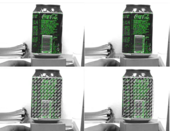
We first assign a regular mesh to the frontal key view (see fig. 1). Then, for each other image of the collection, we compute the best TPS fitting mesh, i.e. the deformation of the regular mesh which minimizes the difference between the key view, after deformation, and the target image.

This estimation is possible once point-to-point correspondences between the key im-age and other training imim-ages are known. We compute these correspondences by detecting and matching key points. These points are detected using Harris and Stephen’s method and represented with SIFT descriptors [9].

Figure 1:Spline deformation after a small rotation of the can. Top : interest points matched using SIFT representation - bottom : estimated mesh deformation.

Even if SIFT based representations are know to produce reliable correspondences, outliers can not be avoided. These outliers dramatically affect the least square estimation of spline parameters. This is why the TPS transformation is computed iteratively using a regularization parameter to relax erroneous matches [17].

The Thine Plate Spline is the Radial Basis Function (RBF) that minimizes the follow-ing bendfollow-ing energy:

If = Z Z

R2( f

2

xx+ 2 fxy2+ fyy2)dxdy

where f = f (x, y) represents the new position of point (x, y) after deformation. The form of f is:

f (x, y) = a1+ axx + ayy + n

∑

i=1

wiU (||(xi, yi) − (x, y)||)

where U (r) = r2log r, a1, ax, ay, wi are the parameters to estimate and (xi, yi) the model

nodes positions.

In the regularized version of TPS fitting, a parameter β in the cost functional controls the trade-off between fitting the data and smoothing :

K[ f ] =

∑

i

(vi− f (xi, yi))2+ β If

where vi represents the transformations target and f (xi, yi) is the new position of point

(xi, yi). This method requires two separable TPS transformations, one for x coordinates

and one for y coordinates.

TPS fitting is applied iteratively several times, starting with high β values. β is de-creased during the iterative process. At each step, the spline is fit using filtered correspon-dences. The distance between a key point and the corresponding key point transformed by the smoothed spline must be below a threshold γ, otherwise it is eliminated for this step. This threshold decreases as β does.

Within three iterations, we generally get a correct alignment. We obtain from this process a deformed mesh that corresponds to the new object appearance in the target image (see fig. 1).

Building a statistical model of deformations Splines can potentially fit almost any shape. However, the set of deformations caused by 3D rotations of the object generally belongs to a smaller subset of these potential deformations. Given a set of appearances and corresponding deformations, we can learn a statistical model that explains these de-formations [3].

We collect m mesh deformations in a matrix M, with one transformation per line. A spline transformation is defined by the position of the n control points, i.e. the position of mesh nodes. M =    x1₁ y1₁ . . . x1_n y1_n .. . xm₁ ym₁ . . . xm_n ym_n   =    g1 .. . gm   

where (xi_j, yi_j) are the coordinates of the jth node of the mesh in the ith image of the collection.

The parameters of the generative model are a = (a1, . . . , aN) with N  n (N will be

defined later); they control the deformations according to

g = g0+ a . Q

where g₀is the mean deformation and Q a matrix describing the variations observed in the training set. This kind of modeling has been extensively used for shape analysis [3].

Q is computed through a principal component analysis (PCA) of M, allowing to find

the underlying low-dimensional manifolds which describe model deformations.

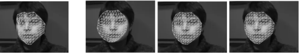
Figure 2: Top left : key view of the object - top right and bottom left : deformations of the key image according to the principal modes of deformation - bottom right : amplification of the deformation

Eigenvectors of a principal component distribution may be separated in two classes. The first one, composed of the N eigenvectors having the largest eigenvalues, represents variations due to the changes in underlying variables. The second are those which can be explained by noise. Different methods can separate these two classes, like the scree-test or the selection of the eigenvalues that express a large amount of the variance.

Given these eigenvectors, mesh deformations can be written as a linear combination of vectors:

g = g0+ a1.e1+ a2.e2+ . . . + ak.ek= g0+ Q . a

where eiis the eigenvector which corresponds to the itheigenvalue.

In the experiments described later, where objects like soda cans or human faces are used to learn proposed tracher, k, the number of selected eigenvectors, is chosen to explain 80% of variance. Its value appeared to be between 2 and 4, depending of tracked object.

It can be seen fig. 2 (top-line) how ajcontrols the deformation of the graph, and

con-sequently the object appearance. If ajis pushed outside of the range of values observed

in the training images, deformations are amplified, as shown fig. 2 (bottom-right). At the end of this stage, we obtain a statistical model of the deformations, character-ized by a mean deformation g0and a linear basis Q.

2.3

Learning to track small patches using linear regressions

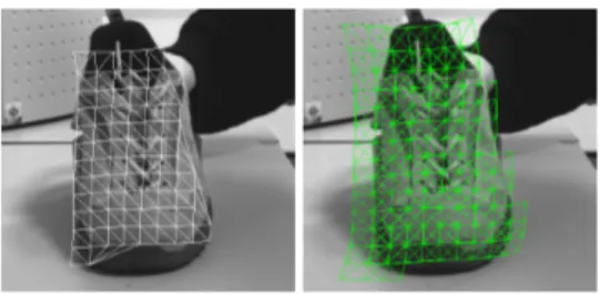
During the tracking stage, mesh deformations will be controlled by local patch corre-spondences. These patches are rectangular regions of the key-view, centered on the mesh nodes. Fig. 3 shows, as an illustration, the patches corresponding to a front key-view of a tracked shoe.

We described in this section an efficient algorithm designed to track these patches.

Figure 3:Patches selected in an old shoe image. left : the mesh - right : mesh and node patches.

The principle of the tracking is as follows. For each patch on the mesh, we learn a linear regressive function by locally perturbing the position of the patch and observing how its texture changes. If V denotes the raw pixel intensities of a patch, and µ its position in the image, the regression can be written [7] as:

δ µ = H . δ v

where H defines the regression to be learned.

H is computed by applying a set of small perturbations δ µ to the original patch

po-sition (i.e. the popo-sition in the key-frame) and observing the difference of pixel intensities (δ v).

The patch’s raw pixel intensities are measured in l points p = (p1, p2, . . . , pl), where

pi= (xi, yi). These coordinates are expressed in the patch reference frame. pipoints are

selected to cover the patch region, at points where image gradient is high [11]. In practice, the patch is split into bins and a given number of points are chosen in each bin.

Let µ(t) = (µ0(t), µ2(t), . . . , µ7(t)) [7] be the vector of parameters describing patch position at time t. They are the parameters of a function which brings points from the ref-erence position to the perturbed position. We use planar patches, so this transformation represents an homography, which is well-known to correspond to the transformation of a planar surface by observed under perspective projection.

During the learning stage, m small perturbations around the initial position are applied to each patch. Let δ v(i) = v(0) − v(i) be the vector of intensity differences, computed as the difference between the initial values and the new values (after the ithperturbation), measured in the key-view. Let δ µ(i) be the vector describing the current perturbation.

H has to verify:

δ µ (i) = H . δ v(i) (1) The aim of the learning stage is to determine H by solving:

   δ µ0(0) . . . δ µm(0) .. . ... δ µ0(p) . . . δ µm(p)   = H.    δ v0(0) . . . δ vm(0) .. . ... δ v0(n) . . . δ vm(n)   

An Himatrix is learned for each patch i. In practice, planar patches are centered on

mesh nodes.

At the end of this stage, one regression per patch has been learned and can be used to obtain patch correspondences over the video sequence.

2.4

Flexible Tracking

Step 1: local correspondences. The first step of the tracking algorithm consists in computing patch correspondences, i.e. mesh nodes correspondences. For each patch of a new frame, we compute the image difference δ v as explained before. Then we obtain

δ µ , which is an estimation of the patch motion parameters, using equation (1).

Using δ µ, we can compute the new position of the center of a patch in the current image, and consequently the new position of the mesh node corresponding to this patch.

Patches are defined as rectangular planar patches of the frontal key-view. However, when the mesh is deformed their shape is obviously also affected by the geometry of the mesh. An homographic transformation is applied to each patch to make them respect global deformation.

It is easy to understand that the complexity of this algorithm is very low: only one ma-trix multiplication and some simple mathematical operations (additions, multiplications, etc.) are necessary to match each patch. It is why we can track many patches almost in real time.

Step 2: estimating the deformations. When each patch position is known in the current frame (step 1), the second step consists in computing the new deformation, using the generative model defined section 2.2.

A Levenberg-Marquardt optimization is used to find the deformation’s parameters which minimize the difference between the positions of the mesh nodes and the corre-sponding patches in the image.

Optimization can be stated as follows. Let pt= (px1t, pyt1, . . . , pxnt, pytn) be the set of

Assuming these notations, the function to be optimized is:

O(c) = ||g0+ Qc − p||

where Q is the statistical model learned offline from training examples. The vector c encodes the deformation of the model for the current frame.

3

Results

We experimented this method with several objects like soda cans, shoes, etc. We focused this section on results obtained for face tracking as well as deformable objects tracking, as both are very challenging problems.

Figure 4:TPS fitting. left : without regularization - right with iterative regularization

Face. The face model was generated using a set of 80 views. The front view was chosen to be the key view. For the 79 other views we used the point correspondence matching algorithm to compute mesh deformations, as previously described.

The number of nodes, for the mesh, was selected in order to have a 1:10 ratio between the number of nodes and the number of point correspondences. It is useless to have more nodes than points correspondences, and this ratio takes into account false matches and non-homogeneous repartition of points.

Figure 5:top : human face tracking - bottom : flexible mouse pad tracking with occultations

As shown in fig 4, a simple TPS computed only from point correspondences does not give accurate results. This is why an iterative algorithm is used. β in this example is set to 1000, 800 and 300 (eq. 2.2).

PCA decomposition and eigenvector selection give the four main underlying param-eters for this model. This model is then used to track the face. Note that this number of

parameters is close to the actual head movements : up/down, left/right, inclination to left and right.

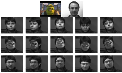
Fig. 6 shows ’augmented’ images; the original face is substituted for a new face taken from a front still image and morphed according to the mesh deformations.

Figure 6:Insertion of two other front images according to model deformations

Deformable objects. Next results, presented fig. 5, illustrate the tracking of deformable surfaces. In this case, patches were located at the 48 nodes of the uniform mesh. During these experiments, we also tried to occlude partially the object and noticed that the algo-rithm was very stable. Without optimizing the code, it takes less than 200 ms per frame to track an object.

4

Conclusions and future works

In this paper, we present a method for fully automatic 3D objects tracking. We show how we can approximate 3D pose changes with 2D spline deformations. Such a flexible model can be automatically learned from a set of images representing appearances of the objects. The proposed method is based on three different principles: fast matching of planar patches, TPS deformations and statistical flexible model learned from of a small training set of object views. This approach is easy to use, does not require any 3D model, and is robust. The local trackers combined with the statistical model of possible deformations make the method fast and very robust to occlusions.

Future works In the future, we will make the tracking stage real-time. We will also extend the proposed works to the tracking of 3D objects using multiple key views. Indeed, the proposed method which is, at the present time, restricted to a single key view does not tolerate large 3D rotations (more than 45 degrees) of the objects.

References

[1] S. Belongie, J. Malik, and J. Puzicha. Shape matching and object recognition using shape contexts. PAMI, 24(4):509–522, April 2002.

[2] D. Comaniciu, V. Ramesh, and P. Meer. Kernel-based object tracking. PAMI, 25(5):564–577, May 2003.

[3] T.F. Cootes, G.J. Edwards, and C.J. Taylor. Active appearance models. PAMI, 23(6):681–685, June 2001.

[4] T.W. Drummond and R. Cipolla. Real-time visual tracking of complex structures. PAMI, 24(7):932–946, July 2002.

[5] G.D. Hager and P.N. Belhumeur. Efficient region tracking with parametric models of geometry and illumination. T-PAMI, 20:1025–1039, 1998.

[6] A.D. Jepson, D.J. Fleet, and T.F. El-Maraghi. Robust online appearance models for visual tracking. PAMI, 25(10):1296–1311, October 2003.

[7] F. Jurie and M. Dhome. Real time tracking of 3d objects: an efficient and robust approach. PR, 35(2):317–328, February 2002.

[8] M. Lades, J.C. Vorbruggen, J. Buhmann, J. Lange, C. von der Malsburg, R.P. Wurtz, and W. Konen. Distortion invariant object recognition in the dynamic link architec-ture. IEEE Transactions on Computers, 42(3):300 – 311, 1993.

[9] David G. Lowe. Object recognition from local scale-invariant features. In Proc. of the International Conference on Computer Vision ICCV, Corfu, pages 1150–1157, 1999.

[10] D.G. Lowe. Fitting parameterized three-dimensional models to images. IEEE Trans. Pattern Analysis and Machine Intelligence, 13(5):441–450, May 1991.

[11] Lucie Masson, Michel Dhome, and Fr´ed´eric Jurie. Robust real time tracking of 3d objects. In ICPR (4), pages 252–255, 2004.

[12] Gabriele Peters. A View-Based Approach to Three-Dimensional Object Perception. PhD thesis, Bielefeld University, 2001.

[13] R. Szeliski and J. Coughlan. Spline-based image registration. IJCV, 22(3):199–218, March 1997.

[14] L. Vacchetti, V. Lepetit, and P. Fua. Stable real-time 3d tracking using online and offline information. PAMI, 26(10):1385–1391, October 2004.

[15] J. Wieghardt, R.P. Wurtz, and C. von der Malsburg. Learning the topology of object views. In ECCV02, page IV: 747 ff., 2002.

[16] J. Wills and S. Belongie. A feature-based approach for determining dense long range correspondences. In ECCV04, pages Vol III: 170–182, 2004.

[17] Josh Wills and Serge Belongie. A feature-based approach for determining long range optical flow. In Proc. European Conf. Comput. Vision, Prague, Czech Republic, May 2004.