A data-driven approach to bucket-filling control for autonomous excavators

A Data-Driven Approach to Bucket-Filling Control

for Autonomous Excavators

by

Ryan Joseph Sandzimier

B.S., University of California, Los Angeles (2015)

Submitted to the Department of Mechanical Engineering

in partial fulfillment of the requirements for the degree of

Master of Science in Mechanical Engineering

at the

MASSACHUSETTS INSTITUTE OF TECHNOLOGY

May 2020

c

○ Massachusetts Institute of Technology 2020. All rights reserved.

Author . . . .

Department of Mechanical Engineering

May 15, 2020

Certified by . . . .

H. Harry Asada

Ford Professor of Engineering

Thesis Supervisor

Accepted by . . . .

Nicolas Hadjiconstantinou

Chairman, Department Committee on Graduate Theses

A Data-Driven Approach to Bucket-Filling Control for

Autonomous Excavators

by

Ryan Joseph Sandzimier

Submitted to the Department of Mechanical Engineering on May 15, 2020, in partial fulfillment of the

requirements for the degree of

Master of Science in Mechanical Engineering

Abstract

We develop a data-driven, statistical control method for autonomous excavators. In-teractions between soil and an excavator bucket are highly complex and nonlinear, making traditional physical modeling difficult to use for real-time control. Here, we propose a data-driven method, exploiting data obtained from laboratory tests. We use the data to construct a nonlinear, non-parametric statistical model for predicting the behavior of soil scooped by an excavator bucket. The prediction model is built for controlling the amount of soil collected with a bucket. An excavator collects soil by dragging the bucket along the soil surface and scooping the soil by rotating the bucket. It is important to switch from the drag phase to the scoop phase with the correct timing to ensure an appropriate amount of soil has accumulated in front of the bucket. We model the process as a heteroscedastic Gaussian process (GP) based on the observation that the variance of the collected soil mass depends on the scooping trajectory, i.e. the input, as well as the shape of the soil surface immediately prior to scooping. We develop an optimal control algorithm for switching from the drag phase to the scoop phase at an appropriate time and for generating a scoop trajectory to capture a desired amount of soil with high confidence. We implement the method on a robotic excavator and collect experimental data. Experiments show promising results in terms of being able to achieve a desired bucket fill factor with low variance. Thesis Supervisor: H. Harry Asada

Acknowledgments

Firstly, I would like to thank my family for the love and support they have given me throughout my life. To my parents, Rick and Kim, thank you for your love and guidance and for shaping me into who I am today. To my siblings, Carter, Tatum, and Garrett, thank you for the countless memories, laughs, and fun we have shared throughout our lives. I am so proud of each of you. To Nana and Papa, thank you for always being there with loving arms for me and the rest of our family.

I would like to thank Brittany Pittner for her support and patience the past couple years. Being away from you has been so hard, but your constant love and encouragement has helped me through it every step of the way. I cannot wait to see what exciting adventures lie ahead for us.

I would also like to thank my advisor, Professor Asada, for his guidance throughout my time at MIT. Thank you for always pushing me to explore new and exciting ideas. I have learned so much from you. Your dedication to your students and our work inspires me.

Lastly, I would like to thank all of my fellow d’Arbeloff lab mates for creating such a friendly and positive environment. Being surrounded by such a talented and motivated group of students and researchers really helped me grow as an engineer. I will always remember the fun times we had both inside and outside of lab.

Contents

2.2 Parameterization of Soil State and Actions . . . 21

3 Prediction and Optimal Control 25 3.1 Prediction Model . . . 25

3.2 Optimal Control . . . 28

4 Experimental Results and Performance 33 4.1 Experimental Setup . . . 33

4.2 Demonstration of Heteroscedasticity . . . 33

4.3 Training the Model . . . 35

4.4 Performance . . . 38

4.5 Discussion . . . 38

List of Figures

1-1 Typical hydraulic excavator (backhoe) used in construction and min-ing industries. In many excavation tasks, the soil medium is fine and homogeneous. . . 14 1-2 The three phases of an excavation cycle (penetrate, drag, scoop). . . . 14 2-1 Three examples of initial soil states. The initial soil state affects the

bucket fill factor and some initial soil states are more desirable. . . . 20 2-2 The (a) mean, (b) first principal component, and (c) second principal

component of the soil state depth maps using principal component analysis. . . 22 2-3 Typical point cloud captured to represent initial soil state . . . 22 2-4 Scoop action parameterization. During the scoop phase, the bucket

rotates about the bucket center (shown as black circle) at a constant velocity. While the bucket rotates, the bucket center moves along a parabolic trajectory. We parameterize the parabolic trajectory 𝑢 = [𝑢1, 𝑢2, 𝑢3]. . . 23

2-5 Drag action parameterization . . . 24 4-1 Experimental setup . . . 34 4-2 Measured bucket fill factor for four groups: long drag and deep scoop

(LD-DS), long drag and shallow scoop (LD-SS), short drag and deep scoop (SD-DS), and short drag and shallow scoop (SD-SS). . . 35 4-3 Normalized mean squared error (NMSE) and normalized log-probability

4-4 Normalized mean squared error (NMSE) and normalized log-probability density (NLPD) for the soil state prediction models. . . 37 4-5 Predicted cost and actual cost at the beginning of the drag phase (top),

after executing one drag action (middle), and after executing a second drag action (bottom). . . 39 4-6 Results controlling the bucket fill factor using the VHGPR (top) and

baseline heuristic (bottom) prediction models to decide when to initiate the scoop phase and which scoop action to perform. There were three target bucket fill factors: 40%, 65%, and 95%. . . 40 4-7 Baseline heuristic method. Volume swept by soil (shaded red) is

List of Tables

Chapter 1

Introduction

1.1

Background

There is a growing need in the construction and mining industries for autonomous excavators that can operate with increased productivity and fuel efficiency [12]. The worldwide shortage of skilled workers to operate these excavators is a major driver behind the development of intelligent excavators for performing various earthmoving tasks.

A single excavation cycle consists of three sequential phases: penetrate, drag, and scoop. Structuring the problem in this way is common practice and breaks the excavation cycle into manageable sub-tasks. First, the bucket penetrates the soil to reach a desirable depth. Next, the bucket moves forward in a dragging motion to accumulate soil inside and in front of the bucket. When a desirable amount of soil has accumulated, the excavator scoops the soil by rotating and translating the bucket to collect the desired amount of soil. Fig. 1-2 illustrates these phases. While loading a dump truck with soil, an experienced operator can fully load the truck in just a few excavation cycles without overloading the truck. This requires the operator to collect a desired amount of soil in the bucket in a limited amount of time. Unskilled operators are unable to precisely fill the bucket, resulting in additional loading cycles and underloading or overloading of the truck. Thus, the amount of soil collected in the bucket, referred to as the bucket fill factor, is a fundamental metric for

Figure 1-1: Typical hydraulic excavator (backhoe) used in construction and mining industries. In many excavation tasks, the soil medium is fine and homogeneous.

Penetrate

Drag

Scoop

Caption: The three phases of an excavation cycle (penetrate, drag, scoop)

Figure 1-2: The three phases of an excavation cycle (penetrate, drag, scoop).

quantifying productivity and operator skill level [5]. Cycle time is another important factor for maximizing productivity. To reduce cycle time and increase fuel efficiency, experienced operators often only fill the bucket to 80% of capacity [12]. Scooping a desired amount of soil is thus a critical requirement for autonomous excavators.

1.2

Prior Work

Early work by Bernold [2] proposed force feedback and impedance control as an effective method for controlling the path of the bucket as it drags through soil. This work focuses mainly on control of the bucket during the drag phase. It does not

consider directly controlling the bucket fill factor, where the scoop phase plays a crucial role. In order to control the bucket fill factor, we must have a model of the bucket-soil interactions. Bucket-soil interactions are very complex and difficult to model. There has been some work using the Fundamental Equation of Earthmoving (FEE) [14] to predict resistive forces during excavation. The FEE relies on parameters that are often unknown a priori. Singh [16] used the FEE to motivate a choice of basis functions to model the resistive forces. They used global regression on a set of training data to determine the coefficients for each of these basis functions. Luengo et. al [10] used a similar data-driven approach, but used gradient descent optimization to directly solve for the nonlinearly involved parameters in the FEE. These data-driven approaches focus on predicting resistive forces. In order to predict the bucket fill factor, we need to be able to predict the actual soil motion during excavation.

Attempts at modeling bucket-soil interactions using discrete-element methods (DEM) are met with computational challenges that make these models infeasible for real-time applications. BLOKS3D [18] is an efficient library for simulating gran-ular particle flow for three-dimensional polyhedral particles of any size. Nezami et. al [11] used this library to simulate bucket-soil interactions during the excavation of coarse gravel. While the results of the simulations were consistent with experimen-tal measurements, the required computation time makes these simulations infeasible for real-time applications with current computer hardware. The simulation required a minimum of 2 hours per second of real time. When using more fine soils, these simulations become even more demanding.

Homma et. al [7] proposed a simple heuristic soil model to apply to the excavation of sand. They discretize the soil volume into a three-dimensional occupancy grid and impose a set of production rules to predict changes to the soil volume’s shape as cells become occupied or vacant. Singh and Simmons [17] used this model for planning ac-tions to take during an excavation cycle. They assume the bucket collects the volume of soil swept by the bucket during an excavation cycle. They then use the production rules to simulate the resettling of the soil after the soil displacement. We use this heuristic model and approach as the baseline when comparing the performance of our

own method.

Singh and Simmons develop a task planning approach to excavation. Placing constraints on the allowable actions of the excavator and forces at the bucket, they choose actions that satisfy a bound on a cost criterion. We propose a similar approach, restricting bucket trajectories to a low-dimensional parameterization that makes the problem tractable. For our approach, the proposed cost criterion to be minimized is related to the bucket fill factor.

1.3

Data-Driven Approach

Terramechanics modeling based on fundamental physical principles is, in general, difficult to use for real-time control due to computational complexity. Model validity is also limited due to unmodeled dynamics. Furthermore, the use of complex feedback control with sophisticated sensors and instrumentation technology is not practical, considering the harsh environment where excavators have to work. In exploring an alternative approach and a new methodology, we exploit the data. Excavation consists mostly of repetitive operations. Although the operations are performed under diverse conditions, we can obtain a large amount of data from both laboratory tests and field operations to handle these conditions. This allows us to use the data for intelligent control of excavators. In a statistical modeling framework, we can deal with highly nonlinear, distributed behaviors of soil without going through terramechanics-based parametric representations. We obtain a non-parametric, nonlinear model directly from the data. It is possible to derive novel control methods from the statistical model.

We aim to apply this data-driven statistical model and control method to bucket fill factor control. The new method takes into account both the expected bucket fill factor as well as the associated variance so we can control the excavator to collect a desired amount of soil with high confidence. Through the estimation of the variance, the data-driven approach can produce a reliable solution to autonomous operation in unstructured environments under diverse conditions.

The method and experiments presented is this thesis are primarily based on work summarized in our previous publication [15].

Chapter 2

Problem Statement

2.1

Bucket Filling Control

The phases of an excavation cycle (penetrate, drag, and scoop) occur sequentially and are dependent on each other. The final conditions after the penetrate and drag phases serve as the initial conditions for the scoop phase. While the scoop phase occurs last chronologically, we choose to focus on it first to better motivate the discussion about the preceding phases later. An excavator can scoop a certain amount of soil by controlling the bucket motion during the scoop phase. However, the amount of scooped soil highly depends on the accumulated soil within the bucket and in front of the bucket just before the scooping action begins. Therefore, the shape of the accumulated soil both inside and in front of the bucket is a critical factor in predicting the bucket fill factor. In the current work, we describe the soil profile with a set of soil state variables, 𝑠 ∈ R𝑛𝑠_{. As detailed later, we measure the accumulated soil with a}

depth camera and compress the image data to a representation using a small number of variables.

The input command to the bucket is described with a vector 𝑢 ∈ R𝑛𝑢 _consisting

of the rotational as well as translational movements of the bucket. In the current work, a single input command defines the entire trajectory of the bucket throughout the scoop phase. The soil profile at the beginning of the scoop phase, 𝑠, and the bucket input command, 𝑢, are the two sets of variables that determine the bucket fill

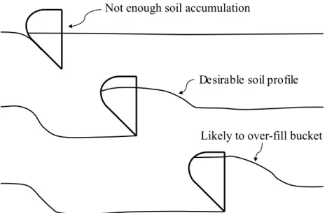
Not enough soil accumulation

Likely to over-fill bucket Desirable soil profile

Figure 2-1: Three examples of initial soil states. The initial soil state affects the bucket fill factor and some initial soil states are more desirable.

factor at the end of the scooping phase. Collectively, these variables are combined as 𝑥 = [𝑠, 𝑢] ∈ R𝑛_{, where 𝑛 = 𝑛}

𝑠+ 𝑛𝑢. The resultant bucket fill factor at the end of

scooping is denoted by output 𝑦.

The bucket fill factor 𝑦 is stochastic. We treat the scoop phase as a stochastic process where the inputs are the combined soil state and bucket command variables, 𝑥, and the output is random variable 𝑦. The bucket fill factor 𝑦 has a probability density conditioned on the soil profile and bucket command, 𝑥.

Fig. 2-1 illustrates three examples of typical soil states. If the scoop is initiated too early (top), we are likely to underfill the bucket. If the scoop is initiated too late (bottom), we will almost surely (low variance) fill the bucket near its capacity for most choices of scoop actions. However, if we only want to fill the bucket partially, say to 80% of its capacity, we are likely to overfill the bucket. For some appropriate transition point (middle), the soil that has accumulated inside and in front of the bucket is desirable and we can likely achieve the desired bucket fill factor. In each case, the soil profile immediately prior to scooping serves as the initial conditions for the scoop phase. As the excavator drags the bucket through the soil, the soil profile continually changes. The excavator controller makes a decision when to initiate the scoop phase by observing the soil profile throughout the drag phase.

To make this control decision, we must construct a prediction model that can predict the bucket fill factor 𝑦* in response to the current soil profile 𝑠* and a bucket

control command 𝑢*. We follow the notation convention from the Gaussian process

regression (GPR) literature by using a * subscript to denote the test inputs and output that we want to make predictions about. If the predicted bucket fill factor is significantly lower than its desired value, the drag phase should continue in hopes of achieving a more desirable 𝑠* in the future. To this end, we must be able to make

predictions about how the soil state will change if the drag action continues. We represent the soil state during the drag phase with a vector 𝑠′ using the same soil state parameterization as before. We represent the drag action as a vector 𝑣 where the elements are the parameter values of the drag action. To condense our notation, we refer to 𝜉 = [𝑠′, 𝑣] as the input vector for the drag phase. Using 𝜉* = [𝑠′*, 𝑣*] to

represent a new test input, we want to make predictions about the corresponding test output 𝑠*. Using such a prediction model, we can make decisions about whether it is

more desirable to initiate the scoop phase using the current soil state or to continue with another drag action and wait to initiate the scoop phase in the future.

2.2

Parameterization of Soil State and Actions

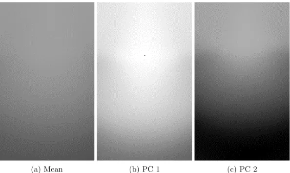
To represent the soil state, we capture a point cloud using a stereo camera. Fig. 2-3 shows a typical point cloud captured during experiments. After isolating points corresponding to the soil inside and in front of the bucket, we project the point cloud onto an orthogonal plane (top) to create a depth map. This depth map contains occlusions, so we use OpenCV [4] to interpolate occlusions using inpainting. This new depth map contains pixels representing the depth of the soil relative to the bucket center. Although the image is high-dimensional due to the large number of pixels, we use principal component analysis and find that the first two principal components explain 96% of the variance in the depth images. Fig. 2-2 shows the mean depth image and the first two principal components of the depth images. We then represent the soil state 𝑠 ∈ R2 as a vector with the projection of the depth image onto the first

(a) Mean (b) PC 1 (c) PC 2

Figure 2-2: The (a) mean, (b) first principal component, and (c) second principal component of the soil state depth maps using principal component analysis.

𝑢₁

𝑢₂

𝑢3

Caption: Scoop action parameterization. During the scoop phase, the bucket rotates about the bucket center (shown as black circle) at a constant velocity. While the bucket rotates, the bucket center moves along a parabolic trajectory. We parameterize the parabolic trajectory 𝑢 = 𝑢1, 𝑢2, 𝑢3 . 𝑢1represents the depth the

bucket center moves downward during the scoop. 𝑢2represents the length traveled in the forward direction

during the scoop. 𝑢3represents the height the bucket center reaches by the end of the trajectory.

Figure 2-4: Scoop action parameterization. During the scoop phase, the bucket ro-tates about the bucket center (shown as black circle) at a constant velocity. While the bucket rotates, the bucket center moves along a parabolic trajectory. We parameterize the parabolic trajectory 𝑢 = [𝑢1, 𝑢2, 𝑢3].

two principal component directions.

To represent the scoop actions, we parameterize the allowable scoop trajectories the bucket follows during scooping. This parameterization is illustrated in Fig. 2-4. During the scoop phase, the bucket rotates about the bucket center to collect the soil. While rotating, we allow the bucket center to follow a parabolic trajectory, which takes three parameters to represent. We find that this parameterization is simple enough to keep the input space relatively small, while also rich enough to allow a sufficient range of scoop actions for controlling the bucket fill factor. We control the bucket along this reference trajectory using impedance control to account for high reaction forces at the bucket that may not allow the robot to follow the reference trajectory exactly.

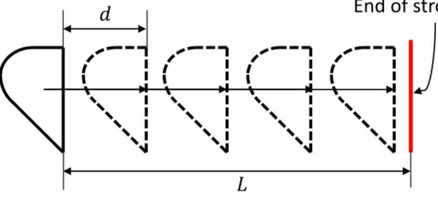
While operators sometimes vary the depth of the bucket throughout the drag, these variations are typically small relative to the forward motion of the bucket. Therefore, we prescribe a constant depth during the drag phase to reduce the di-mensionality of the drag action parameterization. The only parameter necessary to represent a drag action is the drag length, or the distance to move the bucket in the forward direction. The maximum allowable drag length is limited by the workspace

End of stroke

𝐿

𝑑

Figure 2-5: Drag action parameterization

of the excavator. We allow for a discrete set of drag actions 𝑣, represented as:

𝑣 ∈ {𝑑, 2𝑑, . . . , 𝑛𝑑} (2.1)

with integer 𝑛 satisfying 𝑛𝑑 ≤ 𝐿 ≤ (𝑛 + 1)𝑑. 𝑑 is the step size and 𝐿 is the maximum drag length allowed by the workspace of the excavator.

Fig. 2-5 illustrates this parameterization. When optimizing the transition point between the drag phase and scoop phase, we search over the remaining possible drag lengths.

Chapter 3

Prediction and Optimal Control

3.1

Prediction Model

We use a data-driven approach to learn a prediction model. That is, we collect a training data set 𝒟𝑠 = {(𝑥𝑖, 𝑦𝑖)}𝑁𝑖=1 consisting of pairs of inputs and outputs for 𝑁

scoop trials. We model 𝑦 as the sum of some unknown latent function 𝑓 (𝑥) and additive independent noise.

𝑦(𝑥𝑖) = 𝑓 (𝑥𝑖) + 𝜖𝑖 (3.1)

Note that the additive noise 𝜖𝑖 depends on input 𝑥𝑖 because of the heteroscedastic

nature of scooping soil, as discussed previously. We will examine and verify this assumption of heteroscedasticity later in section 4.2.

Given the current test input 𝑥* and the training data set 𝒟𝑠, we must predict

the probability distribution 𝑃 (𝑦*| 𝑥*, 𝒟𝑠) for the corresponding bucket fill factor 𝑦*.

Gaussian processes (GPs) are an effective framework for making this type of pre-diction. Unlike traditional GPs [13], which assume homoscedasticity, our process is heteroscedastic. Goldberg et. al [6] dealt with heteroscedastic GPR (HGPR) using Markov chain Monte Carlo (MCMC) approximate inference. While effective, MCMC is very slow compared to traditional GPR. Lázaro-Gredilla and Titsias [8] developed an effective method called variational HGPR (VHGPR) using a variational approx-imation which maximizes an analytically tractable lower bound on the maximum

likelihood. Lázaro-Gredilla and Titsias have shown that the performance of VHGPR is similar to that of HGPR using MCMC and is comparable in speed to homoscedas-tic GPR. We find VHGPR used for other robohomoscedas-tics applications. Planar pushing, for example, is another problem which exhibits heteroscedastic properties. Bauza and Rodriguez [1] use VHGPR to model and predict the motion of an object being pushed on a planar surface. For a given object state and choice of pushing action, they predict the most likely motion of the object as well as the variability in this motion.

Under the VHGPR framework, we place a GP prior on the latent function 𝑓 (𝑥) and Gaussian priors on the noise terms 𝜖𝑖.

𝑓 (𝑥) ∼ 𝒢𝒫(0, 𝑘𝑓(𝑥, 𝑥′)) (3.2)

𝜖𝑖 ∼ 𝒩 (0, 𝑒𝑔(𝑥𝑖)) (3.3)

where 𝑔(𝑥𝑖) is the log-variance at every input 𝑥𝑖. We also place a GP prior on 𝑔(𝑥).

𝑔(𝑥) ∼ 𝒢𝒫(𝜇0, 𝑘𝑔(𝑥, 𝑥′)) (3.4)

where 𝑘𝑓(𝑥, 𝑥′) and 𝑘𝑔(𝑥, 𝑥′) are covariance functions and 𝜇0 is the noise mean

hyper-parameter. We will explain how we choose 𝜇0 as well as other hyperparameters later

in this section. The covariance functions describe the spatial covariance between any two input vectors 𝑥 and 𝑥′. In practice, we use the automatic relevance determination squared exponential (ARD-SE) kernel for both 𝑘𝑓(𝑥, 𝑥′) and 𝑘𝑔(𝑥, 𝑥′).

𝑘(𝑥, 𝑥′) = 𝜎₀2exp (︃ −1 2 𝑛 ∑︁ 𝑖=1 ([𝑥]𝑖− [𝑥′]𝑖)2 𝑙2 𝑖 )︃ (3.5)

where [𝑥]𝑖 and [𝑥′]𝑖 are the 𝑖𝑡ℎ elements of 𝑥 and 𝑥′, respectively. 𝜎02 and each

𝑙_𝑖2 are hyperparameters for the ARD-SE covariance function. We represent these hyperparameters as a vector Θ = [𝜎2

0, 𝑙12, ..., 𝑙𝑛2]. Covariance functions 𝑘𝑓(𝑥, 𝑥′) and

for 𝑦* according to the VHGPR [8] framework is: 𝑃 (𝑦*| 𝑥*, 𝒟𝑠) = ∫︁ 𝒩 (𝑦*|𝑎*, 𝑐2*+ 𝑒𝑔*)𝒩 (𝑔*|𝜇*, 𝜎*2)𝑑𝑔* (3.6) 𝑎* = 𝑘_{𝑓 *}𝑇 (𝐾𝑓 + 𝑅)−1𝑦 (3.7) 𝑐2_* = 𝑘𝑓 **− 𝑘𝑓 *𝑇 (𝐾𝑓 + 𝑅)−1𝑘𝑓 * (3.8) 𝜇* = 𝑘𝑔*𝑇 (Λ − 1 2𝐼)1 + 𝜇0 (3.9) 𝜎_*2 = 𝑘𝑔**− 𝑘𝑔*𝑇 (𝐾𝑔+ Λ−1)−1𝑘𝑔* (3.10) 𝜇 = 𝐾𝑔(Λ − 1 2𝐼)1 + 𝜇01 (3.11) Σ−1 = 𝐾_𝑔−1+ Λ (3.12)

where 𝑦 is a column vector with elements [𝑦]𝑖 = 𝑦𝑖. 𝐾𝑓 is a matrix with elements

[𝐾𝑓]𝑖𝑗 = 𝑘𝑓(𝑥𝑖, 𝑥𝑗), 𝑘𝑓 * is a column vector with elements [𝑘𝑓 *]𝑖 = 𝑘𝑓(𝑥𝑖, 𝑥*), and

𝑘𝑓 ** = 𝑘𝑓(𝑥*, 𝑥*) for covariance function 𝑘𝑓(𝑥, 𝑥′). We construct 𝐾𝑔, 𝑘𝑔*, 𝑘𝑔** in the

same way using covariance function 𝑘𝑔(𝑥, 𝑥′). 𝑅 is a diagonal matrix with elements

[𝑅]𝑖𝑖 = 𝑒𝑔(𝑥𝑖) where 𝑔(𝑥𝑖) = [𝜇]𝑖 − [Σ]𝑖𝑖/2. 𝑎* and 𝑐2* are the mean and variance

of the predicted latent function 𝑓 (𝑥) at the test input 𝑥*. 𝜇* and 𝜎2* are the mean

and variance of the predicted log-variance function 𝑔(𝑥) at the test input 𝑥*. Λ is

a positive semidefinite diagonal matrix whose elements represent the free parameters in 𝜇 and Σ. We optimize the hyperparameters Λ, 𝜇0, Θ𝑓, and Θ𝑔 simultaneously to

maximize the variational bound.

The predictive distribution in (3.6) is not analytically tractable. However, its mean and variance are computable analytically.

E[𝑦*|𝑥*, 𝒟𝑠] = 𝑎* (3.13)

V[𝑦*|𝑥*, 𝒟𝑠] = 𝑐2*+ 𝑒

𝜇*+𝜎2*/2 _(3.14)

We can use this same framework for making predictions about the soil state 𝑠 throughout the drag phase. Specifically, given a drag test input 𝜉*, we want to make

the soil state 𝑠 is vector-valued. GPR is traditionally formulated only for scalar outputs except for some work [3] that formulates homoscedastic GPs with multiple dependent outputs. To our knowledge, there is no prior work successfully handling heteroscedastic GPs with multiple dependent outputs. In the current work, we make a simplifying assumption that the components of vector 𝑠 are statistically independent and use multiple VHGPR models in parallel to make predictions about each output independently. By making this assumption, we do lose information about potential correlation among outputs. However, we show in Chapter 4 that even with this loss of information we can still make appropriate predictions.

We can make use of (3.1)-(3.14) by substituting 𝜉* for 𝑥*, 𝒟𝑑 = {(𝜉𝑖, 𝑠𝑖)}𝑁𝑖=1 for

𝒟𝑠, and each [𝑠*]𝑗 for 𝑦* and independently optimizing the hyperparameters for each

VHGPR model.

3.2

Optimal Control

In this section, we consider how to optimize our choice of actions given the current soil state and a desired bucket fill factor. To do this, we make use of the prediction models discussed in Section 3.1. First, we focus on the scoop phase. Given the current soil state 𝑠* that we want to test, we choose a trajectory 𝑢𝑜𝑝𝑡 that minimizes a cost

function 𝐶𝑠(𝑠*, 𝑢*).

𝑢𝑜𝑝𝑡 = arg min 𝑢*

𝐶𝑠(𝑠*, 𝑢*) (3.15)

The goal of the scoop phase is to achieve a specified bucket fill factor. A natural choice of cost function is the expected squared error between the bucket fill factor 𝑦*

and some desired bucket fill factor 𝑦𝑑.

𝐶𝑠(𝑠*, 𝑢*) = E[(𝑦*− 𝑦𝑑)2| 𝑥*, 𝒟𝑠] (3.16)

and mean, E[𝑦*2|𝑥*, 𝒟𝑠] = V[𝑦*|𝑥*, 𝒟𝑠] + E[𝑦*|𝑥*, 𝒟𝑠]2 yields:

𝐶𝑠(𝑠*, 𝑢*) = V[𝑦*|𝑥*, 𝒟] + (E[𝑦*|𝑥*, 𝒟] − 𝑦𝑑)2 (3.17)

From (3.13) and (3.14), we have closed-form expressions for the mean and variance that we can plug into (3.17).

𝐶𝑠(𝑠*, 𝑢*) = 𝑐2*+ 𝑒𝜇*+𝜎

2

*/2_{+ (𝑎}

* − 𝑦𝑑)2 (3.18)

To minimize the cost function, we take the derivative with respect to each of the components of the action and use gradient descent methods to search for a minimum. Taking the derivative with respect to [𝑥*]𝑗, the 𝑗𝑡ℎ component of 𝑥* corresponding to

an action input: 𝜕𝐶𝑠(𝑠*, 𝑢*) 𝜕[𝑥*]𝑗 = 𝜕𝑐 2 * 𝜕[𝑥*]𝑗 + (︂ 𝜕𝜇* 𝜕[𝑥*]𝑗 + 1 2 𝜕𝜎2 * 𝜕[𝑥*]𝑗 )︂ 𝑒𝜇*+𝜎2*/2_{+ 2} 𝜕𝑎* 𝜕[𝑥*]𝑗 (𝑎*− 𝑦𝑑) (3.19) 𝜕𝑎* 𝜕[𝑥*]𝑗 = 𝜕𝑘 𝑇 𝑓 * 𝜕[𝑥*]𝑗 (𝐾𝑓 + 𝑅)−1𝑦 (3.20) 𝜕𝑐2 * 𝜕[𝑥*]𝑗 = 𝜕𝑘𝑓 ** 𝜕[𝑥*]𝑗 − 2𝑘𝑇 𝑓 *(𝐾𝑓 + 𝑅)−1 𝜕𝑘𝑓 * 𝜕[𝑥*]𝑗 (3.21) 𝜕𝜇* 𝜕[𝑥*]𝑗 = 𝜕𝑘 𝑇 𝑔* 𝜕[𝑥*]𝑗 (Λ − 1 2𝐼)1 (3.22) 𝜕𝜎2 * 𝜕[𝑥*]𝑗 = 𝜕𝑘𝑔** 𝜕[𝑥*]𝑗 − 2𝑘𝑇_𝑔*(𝐾𝑔+ Λ−1) 𝜕𝑘𝑔* 𝜕[𝑥*]𝑗 (3.23)

where the derivatives of 𝑘𝑓 *, 𝑘𝑔*, 𝑘𝑓 **, 𝑘𝑔** with respect to [𝑥*]𝑗 depend on the

derivatives of the covariance functions. For the ARD-SE covariance functions, we have: [︂ 𝜕𝑘* 𝜕[𝑥*]𝑗 ]︂ 𝑖 = 𝜕𝑘(𝑥𝑖, 𝑥*) 𝜕[𝑥*]𝑗 = [𝑥𝑖]𝑗− [𝑥*]𝑗 𝑙2 𝑗 𝑘(𝑥𝑖, 𝑥*) (3.24) 𝜕𝑘** 𝜕[𝑥*]𝑗 = 𝜕𝑘(𝑥*, 𝑥*) 𝜕[𝑥*]𝑗 = 0 (3.25)

the corresponding cost. To initialize the optimization, we choose a representative sample from the training data set according to a distance metric. Given a current test soil state 𝑠* and a desired bucket fill factor 𝑦𝑑, we choose an optimal scoop

action. However, if the soil state at the start of the scoop phase is undesirable, the cost associated with the optimal scoop may still be high. Therefore, we next consider how to decide if it is better to initiate the scoop phase with the current soil state or to continue the drag action in hopes of making the soil state more desirable prior to scooping.

Given a drag input 𝜉*, we can predict the distribution of the corresponding soil

state output 𝑠*. Rewriting (3.6) in terms of the drag phase inputs and outputs:

𝑃 ([𝑠*]𝑗| 𝜉*, 𝒟𝑑) =

∫︁

𝒩 ([𝑠*]𝑗|𝑎*, 𝑐2*+ 𝑒𝑔*)𝒩 (𝑔*|𝜇*, 𝜎*2)𝑑𝑔* (3.26)

which is analytically intractable. However, we can approximate the distribution up to several digits using Gauss-Hermite quadrature [8], which is computationally inexpen-sive. The accuracy of this approximation is sufficient for our application. In Section 4.5, we discuss the impact of the approximation in further detail.

Using the assumption that the components of the predicted soil state 𝑠* are

statis-tically independent, we can calculate the predicted distribution of the full soil state:

𝑃 (𝑠*|𝜉*, 𝒟𝑑) = 𝑛𝑠 ∏︁ 𝑗=1 𝑃 ([𝑠*]𝑗|𝜉*, 𝒟𝑑) (3.27) where 𝑠* ∈ R𝑛𝑠

In order to make a decision about whether to initiate the scoop phase or continue with another drag action, we must compare the cost to initiate the scoop phase now to the expected cost to initiate the scoop phase in the future. The cost to continue dragging for some drag input 𝜉* is:

𝐶𝑑(𝜉*) = E[𝐶𝑠(𝑠*, 𝑢𝑜𝑝𝑡)|𝜉*, 𝒟𝑑] =

∫︁

𝐶𝑠(𝑠*, 𝑢𝑜𝑝𝑡)𝑃 (𝑠*|𝜉*, 𝒟𝑑)𝑑𝑠* (3.28)

expected cost using importance sampling. While it is difficult to sample directly from 𝑃 (𝑠*|𝜉*, 𝒟𝑑), we can approximate the probability density at a given sample

𝑠*. By sampling from some distribution 𝑞(𝑠*) that is easy to sample from, we can

approximate the expectation as follows:

𝐶𝑑(𝜉*) ≈ 𝑘 ∑︁ 𝑖=1 𝑤(𝑠*,𝑖)𝐶𝑠(𝑠*,𝑖, 𝑢𝑜𝑝𝑡) ∑︀𝑘 𝑖′₌₁𝑤(𝑠*,𝑖′) (3.29) where 𝑤(𝑠*,𝑖) = 𝑃 (𝑠*,𝑖|𝜉*, 𝒟𝑑) 𝑞(𝑠*,𝑖) (3.30) By taking this 𝑘-sample weighted average of the optimal scoop cost, we approxi-mate the cost to continue dragging. The approximation is more accurate for large 𝑘 and in the limit as 𝑘 approaches infinity, the estimated cost approaches the expected cost. In practice, we choose 𝑘 large enough that the approximation is sufficient. In Section 4.5, we discuss this approximation in further detail.

We compare the cost to continue dragging for every possible drag action 𝑣 and compare it to the cost to initiate the scoop phase now. If the cost to initiate scooping is smaller for every choice of 𝑣, we decide to initiate the scoop phase now. Otherwise, we continue dragging by performing one step of a drag action. We then repeat these steps until the scoop phase is initiated.

Chapter 4

Experimental Results and

Performance

In this Chapter, we discuss our experimental implementation of the proposed method and present the experimental results. In addition, we address the assumption of heteroscedasticity in more detail.

4.1

Experimental Setup

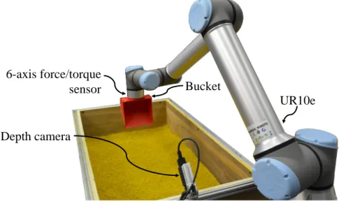
The experimental setup is shown in Fig. 4-1. We use a Universal Robots UR10e to control the excavator bucket. The robot is equipped with a 6-axis force/torque sensor. We use this sensor to measure the mass of soil collected in the bucket after scooping (bucket fill factor). Throughout the dragging phase and immediately prior to scooping, a stereo camera captures a depth image which we use to represent the soil state. The soil medium is homogeneous, low-density, and has particles between 1-3mm in size.

4.2

Demonstration of Heteroscedasticity

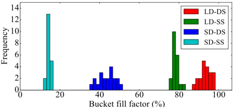
We observe that the variance in the bucket fill factor is dependent on the initial soil state and the chosen scoop action. Fig. 4-2 illustrates this heteroscedastic property.

6-axis force/torque sensor

UR10e Bucket

Depth camera

Figure 4-1: Experimental setup

By measuring the bucket fill factor for repeated trials using the same initial soil state and scoop action, we can test for homoscedasticity. While setting up the exact same initial soil state for repeated trials is not practical, we can achieve approximately the same initial soil state by repeatedly performing a drag trajectory. This is an approximation because repeating a drag trajectory does not guarantee the same soil state. However, we find the approximation is appropriate.

We measure the bucket fill factor for a combination of two separate drag actions and two separate scoop actions. For one of the drag actions, the bucket penetrates deep into the soil and drags for a long length. We refer to this as the long drag. For the other drag action, which we refer to as the short drag, the bucket penetrates to a shallow depth and drags for a short length. During a long drag, a lot of soil accumulates inside and in front of the bucket. On the other hand, for a short drag, the bucket barely moves any soil. We refer to the two choices of scoop actions as the deep scoop and the shallow scoop. For the deep scoop, the bucket moves deep into the soil while also moving forward to collect soil. For the shallow scoop, the bucket only rotates. There is no forward or downward movement during the shallow scoop.

We measure the bucket fill factor for four groups: long drag and deep scoop (LD-DS), long drag and shallow scoop (LD-SS), short drag and deep scoop (SD-(LD-DS), and short drag and shallow scoop (SD-SS). The null hypothesis is that the bucket fill

0 20 40 60 80 100 Bucket fill factor (%)

0 2 4 6 8 10 12 14 Frequency LD-DS LD-SS SD-DS SD-SS

Figure 4-2: Measured bucket fill factor for four groups: long drag and deep scoop (LD-DS), long drag and shallow scoop (LD-SS), short drag and deep scoop (SD-DS), and short drag and shallow scoop (SD-SS).

Table 4.1: p-values of f-tests for comparing sample variances

Samples p-value LD-DS vs. LD-SS 0.0036 LD-DS vs. SD-DS 0.1363 LD-DS vs. SD-SS 1.837 × 10−6 LD-SS vs. SD-DS 2.795 × 10−5 LD-SS vs. SD-SS 0.0280 SD-DS vs. SD-SS 4.816 × 10−9

factor samples came from populations which each have the same variance. We use an F-test to test this hypothesis for each pair of groups. Table 4.1 shows the p-values for each of these tests. We determine with statistical significance that the bucket fill factor is heteroscedastic.

4.3

Training the Model

We collect training data sets 𝒟𝑠and 𝒟𝑑by performing random drag and scoop actions,

measuring the soil state throughout the drag phase and immediately prior to the scoop phase, and measuring the resulting bucket fill factor. The use of random drag and scoop actions provides a rich set of soil states, ensuring the training data set spans the entire input space.

Θ𝑓 and Θ𝑔. In general, we do not know the best choice of hyperparameters, so we

must infer them from the training data. We find the hyperparameters that maximize the variational bound on the log-likelihood [8] using the L-BFGS-B optimization algorithm [19].

We set aside a testing data set to cross-validate the trained prediction models. We use the normalized mean squared error (NMSE) and normalized log-probability density (NLPD) as performance measures. The NMSE and NLPD are defined as follows: 𝑁 𝑀 𝑆𝐸 = ∑︀𝑀 𝑗=1(𝑦*,𝑗 − 𝑎*,𝑗) 2 ∑︀𝑀 𝑗=1(𝑦*,𝑗 − ¯𝑦)2 (4.1) 𝑁 𝐿𝑃 𝐷 = − 1 𝑀 𝑀 ∑︁ 𝑗=1 log(𝑝(𝑦*,𝑗|𝑥*,𝑗, 𝒟𝑠)) (4.2)

where 𝑥*,𝑗 and 𝑦*,𝑗 are the 𝑗𝑡ℎtest input and output, respectively, 𝑀 is the number of

test inputs and outputs, 𝑎*,𝑗 is the mean of the predictive distribution corresponding

to the 𝑗𝑡ℎ _{test input, and ¯𝑦 is the mean of the training data outputs.}

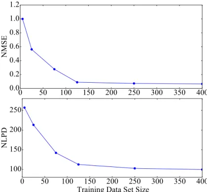
Fig. 4-3 and 4-4 show how the performance measures change with varying training data set sizes for the bucket fill factor prediction model and soil state prediction models, respectively. We find that the performance saturates around 250 training data points for the bucket fill factor prediction model and around 1000 training data points for the soil state prediction models. Beyond this amount of training data, the performance of the models does not seem to improve. Therefore, we train our bucket fill factor prediction model using 250 training data points and our soil state prediction models using 1000 training data points. We observe that the second component of the soil state requires more training data points to saturate than the first component and has a higher NMSE. Since the components of the soil state represent the principal components, it makes sense that the second component would be more difficult to train.

0 50 100 150 200 250 300 350 400 0.0 0.2 0.4 0.6 0.8 1.0 1.2 NMSE 0 50 100 150 200 250 300 350 400

Training Data Set Size 100

150 200 250

NLPD

Figure 4-3: Normalized mean squared error (NMSE) and normalized log-probability density (NLPD) for the bucket fill factor prediction model.

0 200 400 600 800 1000 1200 0.0 0.2 0.4 0.6 0.8 1.0 1.2 NMSE [s]1 [s]2 0 200 400 600 800 1000 1200

Training Data Set Size 2200 2300 2400 2500 2600 2700 2800 NLPD [s]1 [s]2

Figure 4-4: Normalized mean squared error (NMSE) and normalized log-probability density (NLPD) for the soil state prediction models.

4.4

Performance

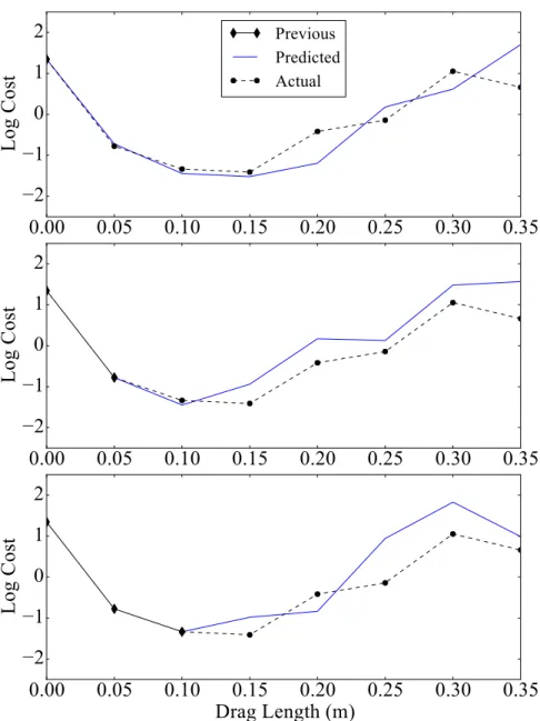
To evaluate the performance of the drag transition decision-making, we measure the cost to initiate the scoop phase throughout the drag phase. Using the prediction model, we decide the optimal transition point. We can then compare this transition point to the actual optimal transition point, which we determine retroactively. Fig. 4-5 shows these results for a single drag phase. We find that the predicted cost is relatively close to the actual measured cost. We illustrate a single drag phase as an example, however, we find these results to be consistent and typical for any choice of target bucket fill factor.

Next, we discuss the performance while controlling the bucket fill factor. We vary the drag depth and target bucket fill factor for each trial and the controller must decide when to transition to the scoop phase and which scoop action to perform to minimize the cost. The varied drag depth provides a variety of initial scenarios which the controller must compensate for. The results of this experiment are shown in Fig. 4-6. We compare our method to a baseline heuristic model [17] that predicts the bucket fill factor by considering the volume of soil swept by the bucket during the excavation cycle. Fig. 4-7 illustrates this volume swept approach that we use as a baseline. We use the same optimization technique to determine the optimal actions when using the heuristic prediction model. For both the VHGPR and heuristic prediction models, as we increase the desired bucket fill factor, the experimentally measured bucket fill factor increases. However, we notice that the results using VHGPR have higher accuracy and lower variance than when using the baseline heuristic model.

4.5

Discussion

In Section 3.2, we present two intractable integrals (3.26) and (3.28) and propose approximations for computing these integrals numerically. We now discuss the ef-fect and suitability of these approximations. When calculating the cost to continue dragging, we approximate the expected cost using a 𝑘-sample weighted average of

0.00 0.05 0.10 0.15 0.20 0.25 0.30 0.35 Drag Length (m) −2 −1 0 1 2 Log Cost Previous Predicted Actual 0.00 0.05 0.10 0.15 0.20 0.25 0.30 0.35 Drag Length (m) −2 −1 0 1 2 Log Cost 0.00 0.05 0.10 0.15 0.20 0.25 0.30 0.35 Drag Length (m) −2 −1 0 1 2 Log Cost

Figure 4-5: Predicted cost and actual cost at the beginning of the drag phase (top), after executing one drag action (middle), and after executing a second drag action (bottom).

0 20 40 60 80 100 Bucket fill factor (%)

0 2 4 6 8 10 Frequency VHGPR 40% Goal 65% Goal 95% Goal 0 20 40 60 80 100

Bucket fill factor (%) 0 2 4 6 8 10 Frequency Baseline Heuristic

Figure 4-6: Results controlling the bucket fill factor using the VHGPR (top) and baseline heuristic (bottom) prediction models to decide when to initiate the scoop phase and which scoop action to perform. There were three target bucket fill factors: 40%, 65%, and 95%.

Figure 4-7: Baseline heuristic method. Volume swept by soil (shaded red) is captured by bucket.

the optimal scoop cost. In the limit as 𝑘 approaches infinity, this sampling-based approach converges to the actual expected cost. One design decision is choosing suffi-ciently large 𝑘 such that the approximation is suitable. In practice, we choose 𝑘 large enough that the approximation is accurate to several digits. In this way, any error introduced from this approximation is negligible compared to errors introduced by process noise, sensor noise, and any model inaccuracies. Similarly, the approximation of probability distributions using Gauss-Hermite quadrature is accurate up to several digits [8], which is more than enough accuracy for our application.

In our experimental implementation, we use a relatively simple parameterization of the action space. It is important to consider how our method scales to more complex parameterizations. As the action space grows, the required training data size tends to increase. Traditional GPs scale as 𝒪(𝑁3_{) with the size of the training}

data [13]. However, there are sparse approximations [9] of GPs, which are more scalable. Determining the optimal transition point between the drag and scoop phases is susceptible to the curse of dimensionality, as is typical for dynamic programming.

Accurate bucket filling is one of the major challenges in autonomous excavation. There is a clear and significant difference even between experienced and novice human operators’ abilities to control the bucket fill factor accurately. Poor bucket-filling accuracy directly influences the overall productivity. The proposed method is the first attempt to fill the gap, and will drive autonomous excavator development to a new level.

Chapter 5

Conclusion

We develop a data-driven model for predicting the bucket fill factor during an exca-vation cycle. Using this prediction model, we develop an optimal control algorithm to determine the optimal transition point between the drag and scoop phases as well as the optimal scoop action to achieve a desired bucket fill factor with high certainty. The experimental results are promising and demonstrate that a data-driven model can be suitable for making predictions about soil-bucket interactions and controlling the bucket fill factor. We present a specific parameterization of the problem, however, the approach extends to other parameterizations if provided an appropriately sized training data set.

There are some key areas for future work on this problem. For the experiment, we used soil of uniform grain size. For real world applications, it is important to consider various soil grain sizes and properties. This requires a large amount of data collected for many different conditions. The proposed GP model is an effective framework. It is flexible enough to apply to the diverse conditions. It is also efficient since it converges with a relatively small training data set size. We use a simple method for parameterizing drag actions, however, considering more complex trajectories may increase the performance.

The proposed method serves as a good low-level controller for controlling bucket fill factor during excavation. However, the approach relies on several high-level pa-rameters such as initial dig location and target bucket fill factor. Therefore, an area

for future work is to combine this approach with a high-level controller that deter-mines these parameters. In this work, the training data sets were collected by uniform randomly sampling the input space. While this helps ensure dense sampling of the input space, it is not data-efficient in the sense that much of the training data will not be in the regions of the input space that would be considered optimal or desir-able. One way to collect a more representative training data set is to use data from expert operation. Therefore, an area of future work is to train models that attempt to emulate expert operators.

Bibliography

[1] Maria Bauza and Alberto Rodriguez. A probabilistic data-driven model for planar pushing. In 2017 IEEE International Conference on Robotics and Au-tomation (ICRA), pages 3008–3015. IEEE, 2017.

[2] Leonhard E Bernold. Motion and path control for robotic excavation. Journal of Aerospace Engineering, 6(1):1–18, 1993.

[3] Phillip Boyle and Marcus Frean. Dependent gaussian processes. In Advances in neural information processing systems, pages 217–224, 2005.

[4] G. Bradski. The OpenCV Library. Dr. Dobb’s Journal of Software Tools, 2000. [5] Siddharth Dadhich, Ulf Bodin, and Ulf Andersson. Key challenges in automation

of earth-moving machines. Automation in Construction, 68:212–222, 2016. [6] Paul W Goldberg, Christopher KI Williams, and Christopher M Bishop.

Regres-sion with input-dependent noise: A gaussian process treatment. In Advances in neural information processing systems, pages 493–499, 1998.

[7] Keiko Homma, Tatsuya Nakamura, Tatsuo Arai, and Hironori Adachi. Spatial image model for manipulation of shape variable objects and application to ex-cavation. In EEE International Workshop on Intelligent Robots and Systems, Towards a New Frontier of Applications, pages 645–650. IEEE, 1990.

[8] Miguel Lázaro-Gredilla and Michalis K Titsias. Variational heteroscedastic gaus-sian process regression. In ICML, pages 841–848, 2011.

[9] Haitao Liu, Yew-Soon Ong, Xiaobo Shen, and Jianfei Cai. When gaussian pro-cess meets big data: A review of scalable GPs. IEEE Transactions on Neural Networks and Learning Systems, 2020.

[10] Oscar Luengo, Sanjiv Singh, and Howard Cannon. Modeling and identification of soil-tool interaction in automated excavation. In Proceedings. 1998 IEEE/RSJ International Conference on Intelligent Robots and Systems. Innovations in The-ory, Practice and Applications (Cat. No. 98CH36190), volume 3, pages 1900– 1906. IEEE, 1998.

[11] Erfan G Nezami, Youssef MA Hashash, Dawei Zhao, and Jamshid Ghaboussi. Simulation of front end loader bucket–soil interaction using discrete element method. International journal for numerical and analytical methods in geome-chanics, 31(9):1147–1162, 2007.

[12] Felix Ng, Jennifer A Harding, and Jacqueline Glass. An eco-approach to op-timise efficiency and productivity of a hydraulic excavator. Journal of cleaner production, 112:3966–3976, 2016.

[13] C. E. Rasmussen and C. K. I. Williams. Gaussian Processes for Machine Learn-ing. MIT Press, 2006.

[14] A. R. Reece. Paper 2: The fundamental equation of earth-moving mechanics. Proc. Inst. Mech. Eng., 179(6):16–22, 1964.

[15] Ryan J Sandzimier and H Harry Asada. A data-driven approach to prediction and optimal bucket-filling control for autonomous excavators. IEEE Robotics and Automation Letters, 5(2):2682–2689, 2020.

[16] Sanjiv Singh. Learning to predict resistive forces during robotic excavation. In Proceedings of 1995 IEEE International Conference on Robotics and Automation, volume 2, pages 2102–2107. IEEE, 1995.

[17] Sanjiv Singh and Reid G Simmons. Task planning for robotic excavation. In IROS, volume 92, pages 1284–1291, 1992.

[18] Dawei Zhao, Erfan G Nezami, Youssef MA Hashash, and Jamshid Ghaboussi. Three-dimensional discrete element simulation for granular materials. Engineer-ing Computations, 23(7):749–770, 2006.

[19] Ciyou Zhu, Richard H Byrd, Peihuang Lu, and Jorge Nocedal. Algorithm 778: L-bfgs-b: Fortran subroutines for large-scale bound-constrained optimization. ACM Transactions on Mathematical Software (TOMS), 23(4):550–560, 1997.