arXiv:1409.5542v2 [hep-ex] 15 Dec 2014
EUROPEAN ORGANISATION FOR NUCLEAR RESEARCH (CERN)
CERN-PH-EP-2014-215
Submitted to: Physical Review D
Search for non-pointing and delayed photons in the diphoton
and missing transverse momentum final state in 8 TeV
pp
collisions at the LHC using the ATLAS detector
The ATLAS Collaboration
Abstract
A search has been performed, using the full data sample of 20.3 fb
−1of 8 TeV proton–proton
col-lisions collected in 2012 with the ATLAS detector at the LHC, for photons originating from a displaced
vertex due to the decay of a neutral long-lived particle into a photon and an invisible particle. The
anal-ysis investigates the diphoton plus missing transverse momentum final state, and is therefore most
sensitive to pair-production of long-lived particles. The analysis technique exploits the capabilities
of the ATLAS electromagnetic calorimeter to make precise measurements of the flight direction, as
well as the time of flight, of photons. No excess is observed over the Standard Model predictions for
background. Exclusion limits are set within the context of Gauge Mediated Supersymmetry Breaking
models, with the lightest neutralino being the next-to-lightest supersymmetric particle and decaying
into a photon and gravitino with a lifetime in the range from 250 ps up to about 100 ns.
c
Search for non-pointing and delayed photons in the diphoton and missing transverse
momentum final state in 8 TeV pp collisions at the LHC using the ATLAS detector
The ATLAS Collaboration
A search has been performed, using the full 20.3 fb−1 data sample of 8 TeV proton–proton collisions collected in 2012 with the ATLAS detector at the LHC, for photons originating from a displaced vertex due to the decay of a neutral long-lived particle into a photon and an invisible particle. The analysis investigates the diphoton plus missing transverse momentum final state, and is therefore most sensitive to pair-production of long-lived particles. The analysis technique exploits the capabilities of the ATLAS electromagnetic calorimeter to make precise measurements of the flight direction, as well as the time of flight, of photons. No excess is observed over the Standard Model predictions for background. Exclusion limits are set within the context of Gauge Mediated Supersymmetry Breaking models, with the lightest neutralino being the next-to-lightest supersymmetric particle and decaying into a photon and gravitino with a lifetime in the range from 250 ps to about 100 ns.
PACS numbers: 12.60.Jv, 13.85.Qk, 13.85.Rm
I. INTRODUCTION
This article reports the results of a search for photons originating from a displaced vertex due to the decay of a neutral long-lived particle into a photon and an invisible particle. The search exploits the capabilities of the AT-LAS liquid-argon (LAr) electromagnetic (EM) calorime-ter to make precise measurements of the flight direction and the time of flight of photons. The analysis uses the full data sample of 8 TeV proton–proton (pp) collisions collected in 2012 with the ATLAS detector at the CERN Large Hadron Collider (LHC), corresponding to an
inte-grated luminosity of 20.3 fb−1. The method used is an
evolution of the ATLAS non-pointing photon analysis [1] using the full 2011 data sample of 7 TeV pp collisions,
cor-responding to an integrated luminosity of 4.8 fb−1. This
previous analysis based on 7 TeV pp collisions found no excess above the Standard Model (SM) background ex-pectation.
Scenarios where neutral long-lived particles are pro-duced in pairs arise naturally, for example, within mod-els of supersymmetry (SUSY) [2–10]. SUSY predicts the existence of a new SUSY partner (sparticle) for each of the SM particles, with identical quantum numbers except differing by half a unit of spin. In R-parity-conserving SUSY models [11–15], pp collisions at the LHC could produce these sparticles in pairs, and they would then decay in cascades involving other sparticles and SM par-ticles until the lightest SUSY particle (LSP) is produced, which is stable. This analysis investigates the diphoton
plus large Emiss
T final state, where EmissT is the
magni-tude of the missing transverse momentum, and is there-fore most sensitive to the pair-production of long-lived particles.
In gauge-mediated supersymmetry breaking (GMSB)
models [16–21], the gravitino ( ˜G) is the LSP and is
predicted, for typical model parameter values, to be very light. While the recent discovery of a Higgs bo-son with a mass around 125 GeV [22, 23] disfavors
minimal GMSB within reach of the LHC, modifications to minimal GMSB can easily accommodate this Higgs mass value without changing the sparticle masses [24– 26]. GMSB phenomenology is largely determined by the properties of the next-to-lightest supersymmetric parti-cle (NLSP), since the decay chains of the spartiparti-cles with higher mass would terminate in the decay of the NLSP. Very weak coupling of the NLSP to the gravitino could lead to displaced decay vertices of the NLSP [20]. The NLSP lifetime (τ ) depends on the fundamental scale of SUSY breaking [27, 28], and therefore provides important information about the SUSY-breaking mechanism.
The results of this analysis are presented within the context of the so-called Snowmass Points and Slopes pa-rameter set 8 (SPS8) [29], which describes a set of
min-imal GMSB models with the lightest neutralino ( ˜χ0
1) as
the NLSP. The free parameter in the GMSB SPS8 set of models is the effective scale of SUSY breaking, denoted Λ, which depends on details of how the SUSY breaking is communicated to the messenger sector of the theory.
For Λ values below about 100 TeV, strong production of pairs of squarks and/or gluinos make a significant con-tribution to the production rate of SUSY events at the LHC. However, for most of the range of Λ values relevant for this analysis, SUSY production is dominated by elec-troweak pair production of gauginos, and in particular of ˜ χ0 2χ˜ ± 1 and ˜χ+1χ˜ − 1 pairs.
In the GMSB SPS8 models, the dominant decay mode
of the NLSP is ˜χ0
1→ γ + ˜G, leading to a γγ +ETmiss+X
fi-nal state, where the escaping gravitinos give rise to Emiss
T ,
and X represents SM particles produced in the decay cas-cades. To minimize the dependence of the results on the details of the SUSY decays, the analysis requires only
a pair of photons and large Emiss
T , avoiding explicit
re-quirements on the presence of leptons or jets or any other particular SM particles in the final state.
This analysis considers the scenario where the NLSP has a finite lifetime, at least 250 ps, and travels part-way through the ATLAS detector before decaying. In
the range of Λ values of interest, about 80–300 TeV, the NLSP mass lies in the range of about 120–440 GeV. In this case, the photons produced in the NLSP decays can either be “non-pointing” or “delayed” or both; namely, the photons can have flight paths that do not point back to the primary vertex (PV) of the event and arrival times at the calorimeter that are later than those expected for a photon produced promptly at the PV.
The search for non-pointing and delayed photons is performed using the excellent performance of the finely segmented LAr EM calorimeters. An EM shower pro-duced by a photon is measured precisely with varying lateral segmentation in three different longitudinal (i.e. depth) segments, allowing a determination of the flight direction of the photon from the EM shower measure-ments. The flight direction can then be compared with the direction back toward the PV identified for the event. This method is employed to determine the value of the
pointing-related variable used, namely |∆zγ|, defined as
the separation, measured along the beamline, between the extrapolated origin of the photon and the position of the selected PV of the event. The LAr calorimeter
also has excellent time resolution and the arrival time tγ
of a photon at the calorimeter (with zero defined as the expected value for a prompt photon from the hard colli-sion) is also a sensitive measure, since positive and finite time values would be expected for photons arising from non-prompt NLSP decays.
In the 7 TeV analysis [1], the pointing measurement was used to extract the result, with the time measure-ment used only qualitatively as a cross-check. The 7 TeV analysis set exclusion limits within the context of GMSB SPS8 models and similar results were obtained in a CMS analysis [30] of their full 7 TeV dataset, but investigating a final state with at least one photon, at least three jets,
and Emiss
T . The current analysis utilizes both the
point-ing and time measurements. As described in Sec. VII, the current analysis divides the sample into six exclusive
categories, according to the value of |∆zγ|, and then
si-multaneously fits the tγ distributions of each of the
cate-gories to determine the possible contribution from signal. The use of both variables greatly improves the sensitivity.
II. THE ATLAS DETECTOR
The ATLAS detector [31] covers nearly the entire solid
angle1 around the collision point and consists of an
in-ner tracking detector surrounded by a solenoid, EM and
1 ATLAS uses a right-handed coordinate system with its origin
at the nominal interaction point (IP) in the center of the de-tector and the z-axis along the beam pipe. The x-axis points from the IP to the center of the LHC ring, and the y-axis points upward. Cylindrical coordinates (r, φ) are used in the trans-verse plane, φ being the azimuthal angle around the beam pipe. The pseudorapidity is defined in terms of the polar angle θ as
η = − ln tan(θ/2), and the transverse energy as ET= E sin θ.
hadronic calorimeters, and a muon spectrometer incorpo-rating three large toroidal magnet systems. The inner-detector system (ID) is immersed in a 2 T axial mag-netic field, provided by a thin superconducting solenoid located before the calorimeters, and provides charged-particle tracking in the pseudorapidity range |η| < 2.5. The ID consists of three detector subsystems, beginning closest to the beamline with a high-granularity silicon pixel detector, followed at larger radii by a silicon mi-crostrip tracker and then a straw-tube-based transition radiation tracker. The ID allows an accurate reconstruc-tion of tracks from the primary pp collision and precise determination of the location of the PV.
This analysis relies heavily on the capabilities of the ATLAS calorimeter system, which covers the pseudo-rapidity range |η| < 4.9. Finely segmented lead/LAr EM sampling calorimeters cover the barrel (|η| < 1.475) and endcap (1.375 < |η| < 3.2) regions. An addi-tional thin LAr presampler covering |η| < 1.8 allows corrections for energy losses in material upstream of the EM calorimeters. Hadronic calorimetry is provided by a steel/scintillator-tile calorimeter, segmented into three barrel structures within |η| < 1.7, and two copper/LAr hadronic endcap calorimeters. The solid angle coverage is completed with forward copper/LAr and tungsten/LAr calorimeter modules, optimized for EM and hadronic measurements, respectively. Outside the calorimeters lies the muon spectrometer, which identifies muons and mea-sures their deflection up to |η| = 2.7 in a magnetic field generated by superconducting air-core toroidal magnet systems.
A. Pointing resolution
For |η| < 2.5, the EM calorimeter is segmented into three layers in depth that are used to measure the longi-tudinal profile of the shower. The first layer uses highly granular “strips” segmented in the η direction, designed to allow efficient discrimination between single photon showers and two overlapping showers, the latter
origi-nating, for example, from the decay of a π0 meson. The
second layer collects most of the energy deposited in the calorimeter by EM showers initiated by electrons or pho-tons. Very high energy showers can leave significant en-ergy deposits in the third layer, which can also be used to correct for energy leakage beyond the EM calorimeter. By measuring precisely the centroids of the EM shower in the first and second EM calorimeter layers, the flight direction of photons can be determined, from which
one can calculate the value of zorigin, defined as the
z-coordinate of the photon projected back to the point giving its distance of closest approach to the beamline (x = y = 0). The angular resolution of the EM calorime-ter’s measurement of the flight direction of prompt tons is about 60 mrad/p(E/GeV), where E is the pho-ton energy. This angular precision corresponds, in the
15 mm for prompt photons with energies in the range of 50–100 GeV. Given the geometry, the z resolution is worse for photons reconstructed in the endcap calorime-ters, so the pointing analysis is restricted to photon can-didates in the EM barrel calorimeter.
In the ATLAS H → γγ analysis [22] that contributed to the discovery of a Higgs boson, this capability of the EM calorimeter was used to help choose the PV from which the two photons originated, thereby improving the diphoton invariant mass resolution and the sensitivity of the search. The analysis described in this paper uses the measurement of the photon flight direction to search for photons that do not point back to the PV. The pointing
variable used in the analysis is ∆zγ, defined as the
dif-ference between zorigin and zPV, the z-coordinate of the
selected PV of the event. Given that zPV is measured
with high precision using the tracker, the zorigin
resolu-tion is essentially equivalent to the resoluresolu-tion in ∆zγ.
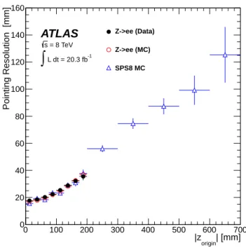
While the geometry of the EM calorimeter is optimized for detecting particles that point back to near the nom-inal interaction point at the center of the detector (i.e. x = y = z = 0), the fine segmentation allows good point-ing performance to be achieved over a wide range of pho-ton impact angles. Figure 1 shows the expected pointing
resolution (ie. the resolution of the measured zorigin) as
a function of |zorigin|, for GMSB SPS8 signal photons in
the EM barrel calorimeter. The results are obtained from Monte Carlo (MC) simulations (see Sec. III) by fitting to a Gaussian function the difference between the
val-ues of zoriginobtained from the calorimeter measurement
and the MC generator-level information. The pointing
resolution degrades with increasing |zorigin|, but remains
much smaller than |zorigin| in the region where the signal
is expected.
The calorimeter pointing performance was verified in data by using the finite spread of the LHC collision region along the z-axis. The pointing resolution achieved for a sample of electrons from Z → ee events is also shown in
Fig. 1, where the distance, zPV, between the PV and the
nominal center of the detector serves the role of zorigin.
In this case, the pointing resolution is obtained by
fit-ting to a Gaussian the difference between zPV, obtained
from reconstructed tracks, and the calorimeter measure-ment of the origin along the beamline of the electron. Figure 1 shows that a similar pointing performance is observed for photons and for electrons, as expected given their similar EM shower developments. This similarity validates the use of a sample of electrons from Z → ee events to study the pointing performance for photons. The expected pointing performance for electrons in a MC sample of Z → ee events is also shown on Fig. 1, and is consistent with the data. The level of agreement between MC simulation and data over the range of values that can be accessed in the data gives confidence in the
extrapo-lation using MC simuextrapo-lation to the larger |zorigin| values
characteristic of signal photons.
| [mm] origin |z 0 100 200 300 400 500 600 700 Pointing Resolution [mm] 0 20 40 60 80 100 120 140 160 Z->ee (Data) Z->ee (MC) SPS8 MC
ATLAS
= 8 TeV s -1 L dt = 20.3 fb∫
FIG. 1. The pointing resolution (defined as the resolution of zorigin) obtained for EM showers in the LAr EM barrel
calorimeter. The pointing resolution for photons from GMSB SPS8 signal MC samples is plotted as a function of |zorigin|.
The pointing resolution is also shown for Z → ee data and MC events, for which the PV position, zPV, serves the role of
|zorigin|.
B. Time resolution
Photons from long-lived NLSP decays would reach the LAr calorimeter with a slight delay compared to prompt
photons produced directly in the hard scatter. This
delay results mostly from the flight time of the heavy NLSP, which would have a distribution of relativistic speed (β = v/c) that peaks typically near 0.9 and has a tail to much lower values. In addition, the opening an-gle in the NLSP decay, which causes the photon to be non-pointing, results in a longer geometrical path to the calorimeter, as compared to a prompt photon from the PV.
The EM calorimeter, with its novel “accordion” de-sign, and its readout, which incorporates fast shaping, has excellent time resolution. Quality-control tests dur-ing production of the electronics required the clock jitter on the LAr readout boards to be less than 20 ps, with typical values of 10 ps [32]. Calibration tests of the over-all electronic readout performed in situ in the ATLAS cavern show a time resolution of ≈ 70 ps [33], limited not by the readout but by the jitter of the calibration pulse injection system. Test-beam measurements [34] of EM barrel calorimeter modules demonstrated a time res-olution of ≈ 100 ps in response to high-energy electrons. The LAr energy and time for each calorimeter cell are reconstructed by applying the optimal filtering al-gorithm [35] to the set of five samples of the signal
shape read out for each calorimeter channel, with suc-cessive samples on the waveform separated by 25 ns. More specifically, the deposited energy per cell and the time of the deposition are calculated using appropriately weighted linear combinations of the set of samples of the waveform: E = 4 X i=0 aiSi and t = 1 E 4 X i=0 biSi , (1)
where Si denotes the five samples of the signal
wave-form. The parameters ai and bi are the optimal filter
coefficients (OFC), the values of which are calculated, knowing the pulse shape and noise autocorrelation ma-trix, to deliver the best energy and time resolutions.
For this analysis, the arrival time of an EM shower is measured using the second-layer EM calorimeter cell with the maximum energy deposit. For the EM shower of an electron or photon with energy within the range of interest, this cell typically contains about (20–50)% of the total energy deposited in the EM shower. In principle, the times measured in neighboring cells could be used in a weighted time calculation to try to further improve the precision. However, some studies that investigated more complicated algorithms found no improvement in time resolution, likely due to the pulse shapes in the channels with lower deposited energies suffering some distortion due to crosstalk effects.
During 2012, the various LAr channels were timed-in online with a precision of order 1 ns. A large sample of W → eν events in the 8 TeV dataset was used to de-termine calibration corrections that need to be applied to optimize the time resolution for EM clusters. The calibration includes corrections of various offsets in the time of individual channels, corrections for the energy dependence of the time measurement, crosstalk correc-tions, and flight-path corrections depending on the PV position.
To cover the full dynamic range of physics signals of interest, the ATLAS LAr calorimeter readout boards [32] employ three overlapping linear gain scales, dubbed High, Medium and Low, where the relative gain is reduced by a factor of about ten for each successive scale. For a given event, any individual LAr readout channel is digitized using the gain scale that provides optimal energy resolu-tion, given the energy deposited in that calorimeter cell. The calibration of the time was determined separately for High and Medium gain for each channel. The num-ber of electron candidates from the W → eν sample that were digitized using Low gain was insufficient to obtain statistically precise results for the calibration constants. Therefore, the analysis requires that selected photons be digitized using either High or Medium gain resulting in a loss in signal efficiency, which ranges from much less than 1%, for the lowest Λ values probed, to less than 5% for the highest Λ values. The majority of signal photons are digitized using Medium gain, the fraction rising with
rising Λ from about 60% to about 90%, over the Λ range of interest.
An independent sample of Z → ee events was used to validate the time calibration and determine the resolution obtained, by performing Gaussian fits to the time distri-butions in bins of cell energy. Figure 2 shows the time resolution for High and Medium gain cells with |η| < 0.4, as a function of the energy in the second-layer calorimeter cell used to calculate the time for the sample of Z → ee events. Similar results are obtained over the full coverage of the EM calorimeter.
Cell Energy [GeV]
10 100 Time Resolution [ns] 0.25 0.30 0.35 0.40 0.45 0.50 0.55 5 20 50 200 = 0.256 1 p = 1.768 0 p |<0.4, High gain η EMB | = 0.299 1 p = 2.550 0 p |<0.4, Medium gain η EMB | -1 Ldt = 20.3 fb
∫
s = 8 TeV ATLASFIG. 2. Time resolution, as a function of the energy in the second-layer cell with the maximum energy, obtained from Z → ee events, for electrons in the EM barrel calorimeter (EMB) with |η| < 0.4, and for both the High and Medium gains. Similar results are obtained over the full coverage of the EM calorimeter. The energy deposited in this cell is typ-ically about (20–50)% of the total energy of the electron. In-cluded in the figure are the results of fitting the time resolu-tion results to the expected form of σ(t) = p0/E ⊕ p1, with
fit parameters p0 (p1) measured in units of GeV·ns (ns). The
time resolution includes a contribution of ≈ 220 ps, which is due to the LHC bunch-spread along the beamline.
The time resolution, σ(t), is expected to follow the
form σ(t) = p0/E ⊕ p1, where E is the cell energy, ⊕
in-dicates addition in quadrature, and the fit parameters p0
and p1are the coefficients of the so-called noise term and
constant term, respectively. Superimposed on Fig. 2 are the results of fits to this expected form of the time
res-olution function. The fits yield values of p1, which gives
the time resolution in the limit of large energy deposits, of 256 ps (299 ps) for High (Medium) gain. The some-what worse results for Medium gain are due to limited statistics in the W → eν sample used to determine the time calibration constants. The time resolution includes a contribution of ≈ 220 ps, which is caused by the time spread in pp collisions for a given PV position due to the
LHC bunch-spread along the beamline. Subtracting this contribution in quadrature implies the LAr contributions to the time resolution are ≈ 130 ps (≈ 200 ps) for High (Medium) gain.
The time resolution is not modeled properly in the MC simulation of the ATLAS detector and it is necessary to apply additional smearing to the MC events in order to match the time performance observed in data. To smear the MC events, the fits to the time resolution determined from Z → ee data as a function of the energy of the most energetic cell in the second layer are used. The fits are parameterized in terms of the pseudorapidity of the cell and the gain scale used to reconstruct the time. To ac-count for the impact of the beam-spread, the smearing includes a component with a Gaussian standard devia-tion of 220 ps that is applied in a correlated way to all photons in the same event. In addition, an uncorrelated component is applied separately to each photon to match its overall time resolution to that observed in data.
C. Measurements of delayed particles
The OFC values in Eq. 1 deviate from being optimal for signals that are early or delayed with respect to the time used to determine the OFC values. This effect can cause the reconstructed values of the energy and time to deviate from their true values.
A source of early and delayed particles can be obtained using so-called satellite bunches of protons that, due to the radio-frequency structure of the LHC accelerator and injection complex, are present in the LHC beams but sep-arated from the main bunches by multiples of ±5 ns. A study was made using W → eν and Z → ee events pro-duced in collisions between pairs of such satellite bunches that occur at the center of the detector but are 5 ns early or late, compared to nominal collisions. These “satellite– satellite” collisions are suppressed in rate by a factor of about one million compared to collisions of the nominal bunches, since the typical population of a satellite bunch is about a factor of one thousand lower than that of the nearby nominal bunch. However, the 8 TeV data sample is sufficiently large that a statistically significant observa-tion of these satellite–satellite collisions could be made.
The values of the mean times reconstructed for elec-trons produced in satellite–satellite collisions were deter-mined to be ≈ −5.1 ns (≈ +5.4 ns), for events that oc-curred 5 ns early (late), demonstrating that the use of fixed OFC values causes a bias for signals that are suf-ficiently early or late compared to the nominal time. In contrast to the time reconstruction, the studies show that the reconstructed energies are very insensitive to modest time shifts of the samples on the waveform, as expected due to the methods used to calculate the OFC values used in the energy calculation. For time shifts within ±5 ns of the nominal time, the reconstructed energy decreases by less than 1%.
III. DATA AND MONTE CARLO SIMULATION SAMPLES
This analysis uses the full dataset of pp collision events
at a center-of-mass energy of√s = 8 TeV, recorded with
the ATLAS detector in 2012. The data sample, after applying quality criteria that require all ATLAS sub-detector systems to be functioning normally, corresponds
to a total integrated luminosity of 20.3 fb−1.
While all background studies, apart from some cross-checks, are performed with data, MC simulations are used to study the response to GMSB signal models, as a function of the free parameters Λ and τ . The other GMSB parameters are fixed to the following SPS8 model
values: the messenger mass Mmess= 2Λ, the number of
SU(5) messengers N5 = 1, the ratio of the vacuum
ex-pectation values of the two Higgs doublets tan β = 15, and the Higgs-sector mixing parameter µ > 0 [29].
The full GMSB SPS8 SUSY mass spectra, branch-ing fractions and decay widths are calculated from this set of parameters using ISAJET [36] version 7.80. The
HERWIG++generator, version 2.4.2 [37], was used to
gen-erate the signal MC samples, with MRST 2007 LO∗
[38] parton density distributions (PDF). A total of 30 signal points, from Λ = 70 TeV to Λ = 400 TeV, were gener-ated, with τ values of 2 ns or 6 ns. For each signal point, 40,000 inclusive GMSB SUSY events were simulated. For each sample, the NLSP was forced to decay to a photon
and gravitino, with the branching fraction BR( ˜χ01→ γ ˜G)
fixed to unity. Other τ values were simulated by appro-priately reweighting the events of these generated sam-ples, with weights related to the decay times of the neu-tralinos, to mimic the expected decay time distributions. Signal cross sections are calculated to next-to-leading order (NLO) in the strong coupling constant using
PROSPINO2 [39]2. The nominal cross section and its
un-certainty are taken from an envelope of cross-section pre-dictions using different PDF sets and factorization and renormalization scales, as described in Ref. [44]. Un-certainties on the cross-section values range from 9% to 14%.
All MC samples used in this analysis were passed through a GEANT4-based simulation [45, 46] of the AT-LAS detector and were reconstructed with the same al-gorithms used for the data. The effect of multiple pp in-teractions in the same or nearby bunch crossings (pileup) is taken into account in all MC simulations and the distri-bution of the number of interactions per bunch crossing in the MC simulation is reweighted to that observed in the data. During the 2012 data-taking period, the av-erage number of pp collisions per bunch crossing varied between 6 and 40, with a mean value of 20.7,
2In addition a resummation of soft gluon emission at
next-to-leading-logarithm accuracy (NLL) [39–43] is performed in the case of strong SUSY pair production.
IV. OBJECT RECONSTRUCTION AND IDENTIFICATION
The reconstruction and identification of electrons and photons are described in Refs. [47, 48] and [49], respec-tively. The photon identification criteria described in Ref. [49] have been re-optimized for the expected pileup conditions of the 8 TeV run period. Shape variables com-puted from the lateral and longitudinal energy profiles of the EM showers in the calorimeter are used to identify photons and discriminate against backgrounds. A set of photon selection criteria, designed for high efficiency and modest background rejection, defines the so-called “loose” photon identification used in this analysis. The loose photon requirements use variables that describe the shower shape in the second layer of the EM calorimeter and leakage into the hadronic calorimeter. These selec-tion criteria do not depend on the transverse energy of
the photon (ET), but do vary as a function of η in order
to take into account variations in the calorimeter geome-try and upstream material. The efficiency of these loose requirements, for the signal photons, is over 95% over
the range |zorigin| < 250 mm and steadily falls to
approx-imately 75% at |zorigin| = 700 mm.
The measurement of Emiss
T [50] is based on the energy
deposits in the calorimeter with |η| < 4.9 and the en-ergy associated with reconstructed muons; the latter is estimated using the momentum measurement of its re-constructed track. The energy deposits associated with
reconstructed objects (jets defined using the anti-kt
algo-rithm [51] with radius parameter 0.4, photons, electrons) are calibrated accordingly. Energy deposits not associ-ated with a reconstructed object are calibrassoci-ated accord-ing to their energy sharaccord-ing between the EM and hadronic calorimeters.
V. EVENT SELECTION
The selected events were collected by an online trigger requiring the presence of at least two loose photons with
|η| < 2.5, one with ET > 35 GeV and the other with
ET > 25 GeV. This trigger is insensitive to the time of
arrival of photons that are relevant for the signal consid-ered, but there may be a slight dependence of the trigger
efficiency on the zoriginof the photon. This effect is
dis-cussed in Sec. VIII A. The trigger efficiency exceeds 99% for signal events that pass the offline selection cuts. To ensure the selected events resulted from a pp collision, events are required to have at least one PV candidate with five or more associated tracks, each with transverse
momentum satisfying pT> 400 MeV. In case of multiple
vertices, the PV is chosen as the vertex with the great-est sum of the squares of the transverse momenta of all associated tracks.
The offline photon selection requires two loose photons
with ET> 50 GeV and |η| < 2.37 (excluding the
transi-tion region between the barrel and endcap EM
calorime-ter at 1.37 < |η| < 1.52). At least one photon is required to be in the barrel region |η| < 1.37. Both photons are required to be isolated, by requiring that the transverse energy deposited in the calorimeter in a cone of radius
∆R =p(∆η)2+ (∆φ)2 = 0.4 around each photon
can-didate be less than 4 GeV, after corrections to account for pileup and the energy deposition from the photon itself [49]. To avoid collisions due to satellite bunches, both photons are required to have a time that satisfies
|tγ| < 4 ns.
The selected diphoton sample is divided into exclusive
subsamples according to the value of Emiss
T . The
sub-sample with ETmiss< 20 GeV is used to model the prompt
backgrounds, as described in Sec. VI B. The events with
20 GeV < Emiss
T < 75 GeV are used as control samples to
validate the analysis procedure and background model.
Diphoton events with Emiss
T > 75 GeV define the signal
region.
Table I summarizes the total acceptance times ef-ficiency of the selection requirements for examples of GMSB SPS8 signal model points with various Λ and τ values. Strong SUSY pair production is only significant for Λ <100 TeV. For Λ = 80 TeV and τ = 6 ns, the acceptance times efficiency is evaluated from MC sam-ples to be 1.6 ± 0.1% and 2.1 ± 0.1% for weak and strong production, respectively, corresponding to a total value of 1.7 ± 0.1%. For fixed Λ, the acceptance falls approx-imately exponentially with increasing τ , dominated by the requirement that both NLSP decay before reaching the EM calorimeter, so that the resulting photons are de-tected. For fixed τ , the acceptance increases with increas-ing Λ, since the SUSY particle masses increase, leadincreas-ing
the decay cascades to produce, on average, higher Emiss
T
and also higher ET values of the decay photons.
TABLE I. The total signal acceptance times efficiency, given in percent, of the event selection requirements, for sample GMSB SPS8 model points with various Λ and τ values. The uncertainties shown are statistical only.
τ Signal acceptance times efficiency [%] [ns] Λ = 80 TeV Λ = 160 TeV Λ = 320 TeV
0.5 8.4 ± 0.6 30 ± 1 46 ± 2 2 5.1 ± 0.3 21 ± 0.2 33.0 ± 0.3 6 1.7 ± 0.1 7.3 ± 0.1 12.5 ± 0.2 10 0.86 ± 0.03 3.71 ± 0.06 6.45 ± 0.09 40 0.089 ± 0.004 0.38 ± 0.01 0.70 ± 0.02 100 0.016 ± 0.001 0.070 ± 0.002 0.129 ± 0.004
VI. SIGNAL AND BACKGROUND MODELING
The analysis exploits both the pointing and time mea-surements. However, the measured properties of only one of the two photons are used, where the choice of which
photon to use is made according to the location of the two photons. The selection requires at least one of the photons to be in the barrel region, since events with both photons in the endcap calorimeters are expected to con-tribute very little to the signal sensitivity. For events, referred to hereafter as BE events, where one photon is found in the barrel and one in the endcap calorimeter,
the ∆zγ and tγ measurements of the barrel photon are
used in the analysis; this choice is made since, due to
geometry, the ∆zγ resolution in the barrel calorimeter is
better. For so-called BB events, with both photons in the
EM barrel calorimeter, the ∆zγ and tγ measurements of
the photon with the maximum value of tγare used.
Stud-ies showed that this approach achieves a sensitivity very similar to that when using both photons, while avoiding the complexity of having to deal with the correlations between the measurements of the two photons within a single event.
A. GMSB SPS8 signal
The shape of the ∆zγ and tγ distributions for signal
events is obtained from the signal MC samples. For a given value of Λ, the distributions for any NLSP lifetime value can be obtained by appropriately reweighting the distributions of the existing MC samples.
Examples of ∆zγ and tγ signal distributions for a few
representative GMSB SPS8 models are shown in Fig. 3. The distributions are normalized to unity area within the displayed horizontal-axis range, in order to allow for an easier comparison between the various signal and back-ground shapes. The upper two plots show signal shapes for some example NLSP lifetime (τ ) values, all with Λ fixed to a value of 160 TeV. The lower two plots show sig-nal shapes for some example Λ values, all with τ fixed to a value of 1 ns. The signal shapes have some dependence on Λ due to its impact on the SUSY mass spectrum, and therefore the event kinematics. However, the signal shapes vary most strongly with NLSP lifetime. For larger τ values, the signal shapes are significantly impacted by the diphoton event selection, which effectively requires that both NLSP decay before reaching the EM calorime-ters, leading to a signal acceptance that falls rapidly with increasing time values. As a result, the signal shapes for τ values of 2.5 ns and 25 ns, for example, are quite simi-lar, as shown in the upper plots of Fig. 3.
B. Backgrounds
The background is expected to be completely domi-nated by pp collision events, with possible backgrounds due to cosmic rays, beam-halo events, or other non-collision processes being negligible. The source of the loose photons in background events contributing to the selected sample is expected to be either a prompt photon, an electron misidentified as a photon, or a jet
misidenti-fied as a photon. In each case, the object providing the loose photon signature originates from the PV.
The pointing and time distributions expected for the background sources are determined using control sam-ples in data. In addition to avoiding a reliance on the precise MC simulation of the pointing and timing per-formance for the backgrounds, and particularly of the
tails of their ∆zγ and tγ distributions, using data
sam-ples naturally accounts for the influence of pile-up, the possibility of selecting the wrong PV, and any instrumen-tal or other effects that might influence the background measurements.
Given their similar EM shower developments, the pointing and time resolutions for prompt photons are
similar to those for electrons. The tγ distribution in each
∆zγ category is modeled using electrons from Z → ee
data events. The Z → ee event selection requires a pair of oppositely charged electron candidates, each of which
has pT> 35 GeV and |η| < 2.37 (excluding the
transi-tion region between the barrel and endcap calorimeters). Both electrons are required to be isolated, with the trans-verse energy deposited in the calorimeter in a cone of size ∆R = 0.2 around each electron candidate being less than 5 GeV, after subtracting the energy associated with the electron itself. As for photons, electrons must be read out using either High or Medium gain, and must have a time less than 4 ns. The dielectron invariant mass is required to be within 10 GeV of the Z boson mass, yielding a suf-ficiently clean sample of Z → ee events. The electrons
are used to construct ∆zγ and tγ templates. The
unit-normalized Z → ee templates are shown superimposed on the plots of Fig. 3.
Due to their wider showers in the EM calorimeter, jets
have a wider ∆zγ distribution than prompt photons and
electrons. Events passing the diphoton selection with
Emiss
T < 20 GeV are used as a data control sample that
includes jets with properties similar to the background
contributions expected in the signal region. The Emiss
T
re-quirement serves to render negligible any possible signal contribution in this control sample. The time resolution depends on the deposited energy in the calorimeter.
Us-ing the shape of the Emiss
T < 20 GeV template to describe
events in the signal region, defined with Emiss
T > 75 GeV
therefore implicitly relies on the kinematic distributions for photons in both regions being similar. However, it is expected that there should be a correlation between the
value of Emiss
T in a given event, and the ET distribution
of the physics objects in that event. This correlation is
indeed observed in the low-Emiss
T control region samples.
Increasing to 60 GeV the minimum ET requirement on
the photons in the Emiss
T < 20 GeV control sample selects
photons with similar kinematic properties to the photons
in the signal region. Therefore, the Emiss
T < 20 GeV
sam-ple requiring ET > 60 GeV for the photons is used to
model the background.
The selected diphoton sample with Emiss
T < 20 GeV
should be dominated by jet–jet, jet–γ and γγ events.
[mm] γ z ∆ -2000 -1500 -1000 -500 0 500 1000 1500 2000 Normalized Entries/40 mm -5 10 -4 10 -3 10 -2 10 -1 10 1 miss < 20 GeV T Data E ee → Data Z = 0.25 ns τ = 160 TeV Λ = 1 ns τ = 160 TeV Λ = 2.5 ns τ = 160 TeV Λ = 25 ns τ = 160 TeV Λ
ATLAS
= 8 TeV s -1 L dt = 20.3 fb∫
[ns] γ t -4 -3 -2 -1 0 1 2 3 4 Normalized Entries/200 ps -4 10 -3 10 -2 10 -1 101 Data EmissT < 20 GeV
ee → Data Z = 0.25 ns τ = 160TeV Λ = 1 ns τ = 160TeV Λ = 2.5 ns τ = 160TeV Λ = 25 ns τ = 160TeV Λ
ATLAS
= 8 TeV s -1 L dt = 20.3 fb∫
[mm] γ z ∆ -2000 -1500 -1000 -500 0 500 1000 1500 2000 Normalized Entries/40 mm -5 10 -4 10 -3 10 -2 10 -1 10 1 miss < 20 GeV T Data E ee → Data Z = 1 ns τ = 80 TeV Λ = 1 ns τ = 160 TeV Λ = 1 ns τ = 300 TeV ΛATLAS
= 8 TeV s -1 L dt = 20.3 fb∫
[ns] γ t -4 -3 -2 -1 0 1 2 3 4 Normalized Entries/200 ps -4 10 -3 10 -2 10 -1 10 1 miss < 20 GeV T Data E ee → Data Z = 1 ns τ = 80TeV Λ = 1 ns τ = 160TeV Λ = 1 ns τ = 300TeV ΛATLAS
= 8 TeV s -1 L dt = 20.3 fb∫
FIG. 3. Signal distributions for (left) ∆zγ and (right) tγ, for some example GMSB SPS8 model points. The upper two plots
show signal shapes for NLSP lifetime (τ ) values of 0.25, 1, 2.5, and 25 ns, all with the effective scale of SUSY breaking (Λ) fixed to a value of 160 TeV. The lower two plots show signal shapes for Λ values of 80, 160, and 300 TeV, all with τ fixed to a value of 1 ns. Superimposed on each of the plots are the corresponding data distributions for the samples used to model the backgrounds, namely Z → ee events and diphoton events with Emiss
T < 20 GeV. For all plots, the distributions are normalized
to unity area within the horizontal-axis range displayed, and the uncertainties shown on the data distributions are statistical only.
clude contributions from photons as well as from misiden-tified jets that satisfy the loose photon signature. The
unit-normalized Emiss
T < 20 GeV templates are shown
superimposed on the plots of Fig. 3. As expected, Fig. 3
shows that the ∆zγ distribution is much wider for the
Emiss
T < 20 GeV sample than for the Z → ee
sam-ple, while the tγ distributions of these two background
samples are very similar. Both backgrounds have
distri-butions that are very different than those expected for GMSB SPS8 signal events, with larger differences ob-served for higher lifetime values.
VII. STATISTICAL ANALYSIS
The photon pointing and time measurements are each sensitive to the possible presence of photons from dis-placed decays of heavy, long-lived NLSP. In addition,
the measurements of ∆zγ and tγ are almost completely
uncorrelated for prompt backgrounds. The lack of
cor-relation results from the fact that ∆zγ uses the spread
of the EM shower to precisely measure its centroids in
the first two layers in the EM calorimeter, while tγ uses
the time reconstructed from the pulse-shape of only the second-layer cell with the maximum energy deposit. Us-ing both variables to distUs-inguish signal from background is therefore a powerful tool.
Since the ∆zγ distribution should be symmetric for
both signal and background, the pointing distribution is
folded by taking |∆zγ| as the variable of interest instead
of ∆zγ. The inputs to the statistical analysis are,
there-fore, the values of |∆zγ| and tγ measured for the photon
selected in each event.
A full two-dimensional (2D) analysis of |∆zγ| versus
tγ would require populating a very large number of bins
of the corresponding 2D space with both the background and signal models. Since the background model is deter-mined using data in control samples, which have limited numbers of events, this approach is impractical. Instead, the original 2D analysis is transformed into a “N × 1D”
problem by using the |∆zγ| values to define N mutually
exclusive categories of photons, and then simultaneously
fitting the tγ spectra of each of the categories. To
op-timize the sensitivity of the analysis, the categories are chosen to divide the total sample of photons into cat-egories with different signal-to-background ratios. This approach is similar to that followed in the ATLAS deter-mination of the Higgs boson spin in the H → γγ decay channel [52].
An additional motivation for applying the “N × 1D” approach is to simplify the task of modeling the over-all background with an unknown mixture of the back-ground templates measured using the Z → ee and
Emiss
T < 20 GeV samples. As shown in Fig. 3, these
sam-ples used to model the various background contributions
have different |∆zγ| distributions, but very similar tγ
dis-tributions. The minor tγ differences can be handled, as
described in Sec. VIII, by including a small systematic
uncertainty on the tγ background shape. However, the
|∆zγ| distribution of the total background depends
sensi-tively on the background composition. By implementing
the normalization of the background in each |∆zγ|
cate-gory as an independent, unconstrained nuisance param-eter, the fitting procedure eliminates the need to predict
the overall |∆zγ| distribution of the total background,
thereby avoiding the associated dependence on knowl-edge of the background composition.
The binning in both |∆zγ| and tγ was chosen to
op-timize the expected sensitivity. It was found that using
six |∆zγ| categories and six tγ bins provides the analysis
with good expected sensitivity, without undue
complex-ity. While the optimized choice of bin boundaries has almost no dependence on Λ, there is some dependence on NLSP lifetime. The analysis, therefore, uses two separate choices of binning, one for low lifetime values (τ < 4 ns) and one for high lifetime values (τ > 4 ns). The op-timized category and bin boundaries for both cases are summarized in Tables II and III, respectively.
The one-dimensional fits of the tγ distributions of the
individual categories are performed simultaneously. The signal normalization is represented by a single uncon-strained signal-strength parameter, µ, that is correlated between all categories and defined as the fitted signal cross section divided by the GMSB SPS8 prediction. Thus, there are seven unconstrained parameters in the fit, namely six separate nuisance parameters, one for each category, describing the background normalization, and the signal strength µ.
The analysis uses a likelihood model L(µ, θ) that is de-pendent on the signal strength µ and the values of the nuisance parameters θ. The model incorporates a statis-tical Poisson component as well as Gaussian constraint terms for the nuisance parameters associated with sys-tematic uncertainties. The statistical model and pro-cedure are implemented within the HistFactory
frame-work [53]. Two likelihood-based test statistics q0and qµ
are calculated to find the p0 values for the
background-only hypothesis and to set upper limits on the signal strength.
Asymptotic formulae based on Wilk’s theorem are used
to approximate the q0 and qµ distributions following the
procedures documented in Ref. [54]. Tests of the back-ground model’s validity in the control regions and the
signal region rely on the p0test statistic, calculated from
the observed q0. In the absence of any excess, the CLS
exclusions for each signal type are calculated according to Ref. [55].
To validate the statistical model and asymptotic forms
of q0 and qµ, unconditional pseudo-experiment
ensem-bles were generated from the background-only model and multiple signal-plus-background models. Although the number of data events in the signal region is not
large, deviations from the asymptotic χ2 distribution of
qµwere shown to have a minimal impact on the exclusion.
The model accurately reconstructed the signal and back-ground normalization parameters and produced Gaus-sian distributions of the constrained nuisance parame-ters.
VIII. SYSTEMATIC UNCERTAINTIES
In the statistical analysis, the background
normaliza-tion for each |∆zγ| category is determined using an
in-dependent nuisance parameter. Therefore, it is not nec-essary to include systematic uncertainties regarding the normalization of the background, nor regarding its shape
in the variable |∆zγ|. As a result, the various
TABLE II. Values of the optimized ranges of the six |∆zγ| categories, for both low and high NLSP lifetime (τ ) values.
NLSP Range of |∆zγ| values for each category [mm]
Lifetime Cat. 1 Cat. 2 Cat. 3 Cat. 4 Cat. 5 Cat. 6 τ < 4 ns 0 – 40 40 – 80 80 – 120 120 – 160 160 – 200 200 – 2000 τ > 4 ns 0 – 50 50 – 100 100 – 150 150 – 200 200 – 250 250 – 2000
TABLE III. Values of the optimized ranges of the six tγbins, for both low and high NLSP lifetime (τ ) values.
NLSP Range of tγ values for each bin [ns]
Lifetime Bin 1 Bin 2 Bin 3 Bin 4 Bin 5 Bin 6 τ < 4 ns −4.0 – +0.5 0.5 – 1.1 1.1 – 1.3 1.3 – 1.5 1.5 – 1.8 1.8 – 4.0 τ > 4 ns −4.0 – +0.4 0.4 – 1.2 1.2 – 1.4 1.4 – 1.6 1.6 – 1.9 1.9 – 4.0
into two categories: so-called “flat” uncertainties are not
a function of |∆zγ| and tγ and affect only the overall
sig-nal yield, while “shape” uncertainties are those that are
related to the shapes of the unit-normalized |∆zγ| and tγ
distributions for signal or to the shape of the background
tγ template.
A. Signal yield systematic uncertainties
The various flat systematic uncertainties affecting the signal yield are summarized in Table IV. The uncertainty on the integrated luminosity is ±2.8% and is determined with the methodology detailed in Ref. [56]. The un-certainty due to the trigger is dominated by
uncertain-ties on the dependence on |∆zγ| of the efficiency of the
hardware-based Level 1 (L1) trigger. The L1 calorime-ter trigger [57] uses analog sums of the channels grouped within projective trigger towers. This architecture leads to a small decrease in L1 trigger efficiency for highly non-pointing photons, due to energy leakage from the relevant trigger towers. The uncertainty on the impact of this de-pendence is conservatively set to the magnitude of the observed change in efficiency in signal MC events versus
|∆zγ|, and dominates the ±2% uncertainty on the trigger
efficiency.
Following the method outlined in Ref. [58], uncertain-ties on the signal efficiency, arising from the combined im-pact of uncertainties in the photon energy scale and reso-lution and in the combined photon identification and iso-lation efficiencies, are determined to be ±1% and ±1.5%, respectively. An additional 4% is included as a conser-vative estimate of the uncertainty in the identification efficiency due to the non-pointing nature of the photons. This estimate is derived from studies of changes in the rel-evant variables measuring the shapes of the EM showers for non-pointing photons. An uncertainty on the signal
yield of ±1.1% results from varying the Emiss
T energy scale
and resolution within their estimated uncertainties [50]. The uncertainty on the signal efficiency due to MC statis-tics lies in the range ±(0.8–3.6)% and the contribution due to the lifetime reweighting technique is in the range
±(0.5–5)%, depending on the sample lifetime.
Variations in the calculated NLO signal cross sections times the signal acceptance and efficiency, at the level of ±(9 − 14)% occur when varying the PDF set and factor-ization and renormalfactor-ization scales, as described in Sec. III. In the results, these uncertainties on the theoreti-cal cross section are shown separately, as hashed bands around the theory prediction. Limits are quoted at the points where the experimental results equal the value of the central theory prediction minus one standard devia-tion of the theoretical uncertainty.
TABLE IV. Summary of relative systematic uncertainties that affect the normalization of the signal yield. The last row summarizes the relative uncertainty on the theoretical cross section, and is treated separately, as explained in the text.
Source of uncertainty Value [%] Integrated luminosity ± 2.8 Trigger efficiency ± 2 Photon ETscale/resolution ± 1
Photon identification and isolation ± 1.5 Non-pointing photon identification ± 4 Emiss
T reconstruction ± 1.1
Signal MC statistics ± (0.8–3.6) Signal reweighting ± (0.5–5) Signal PDF and scale uncertainties ± (9–14)
B. Signal shape systematic uncertainties
The expected signal distributions are determined us-ing the GMSB SPS8 MC signal events. Therefore, lim-itations in the MC simulation could lead to differences between data and MC events in the predicted signal be-havior. Any such discrepancies in the shapes of the signal distributions must be handled by corresponding sysatic uncertainties on the signal shapes. Since signal
analysis, systematic uncertainties on the signal shapes of both must be taken into account in the fitting procedure. The dominant systematic uncertainty on the shape of
the signal tγ distribution arises from the impact of the
time reconstruction algorithm on the measurement of de-layed signals. As discussed in Sec. II C, the use of fixed OFC values causes a bias in the energy and time recon-structed for signals that are sufficiently early or late com-pared to the nominal time. For time shifts within ±5 ns of the nominal time, the reconstructed energy decreases by less than 1% and, as a result, impacts on the measure-ments of the photon energy and pointing are negligible. However, for time shifts of ±5 ns, a bias in the time re-construction of order 10% of the shift is observed in the analysis of satellite–satellite collisions. Since the optimal filtering approach is equivalent to a linearization of the optimization problem, the expected form of the time bias is expected to be dominated by the neglected quadratic terms in the Taylor expansion. Therefore, one expects deviations in the time measurement to be small for small time shifts, over a region where the linear approxima-tion works well, and then to grow roughly quadratically for larger time shifts. As a conservative estimate of the systematic uncertainty on the time measurement due to these effects, a linear dependence is assumed for the devi-ations, with an amplitude of ±10% of the reconstructed time. This uncertainty is applied only to the signal time distribution, since the background time shape is deter-mined directly from data and therefore already includes whatever impact is caused by the bias.
Another source of systematic uncertainty in the signal
|∆zγ| and tγ shapes results from possible differences
be-tween the pileup conditions in data and signal MC events, even though the MC signal samples are reweighted to match the pileup distribution observed in the data. The PV in GMSB SPS8 signal events should be correctly iden-tified with high efficiency, typically greater than 90%,
due to the high ETvalues of the other SM particles
pro-duced in the SUSY decay chains. However, the presence of pileup could still increase the likelihood of incorrectly choosing the PV, potentially impacting both the point-ing and time measurements. Nearby energy deposits that are not associated with the photon could also impact the photon measurements, though these should be moder-ated by the photon isolation requirements. As a conser-vative estimate of the possible influence of pileup, the signal shapes in the entire MC sample were compared with those in two roughly equally sized subsamples with differing levels of pileup, chosen as those events with less than, and those with greater than or equal to, 13 recon-structed PV candidates. The small differences observed are included as pileup-induced systematic uncertainties on the signal template shapes.
To investigate the possible impact of the imperfect knowledge of the material distribution in front of the calorimeter, one signal MC point was simulated with the nominal detector description as well as with a modified version that varies the material description within the
un-certainties. The signal distributions using the two detec-tor geometries are very similar, typically agreeing within a few percent. These variations are small compared to the other systematic uncertainties on the signal shapes, and are therefore neglected.
Typical values of the total systematic uncertainties on the signal shapes are around ±10%, dominated by the impact of the time reconstruction algorithm on the mea-surement of delayed signals. These uncertainties have a very small impact on the overall sensitivity of the analy-sis, which is dominated by statistical uncertainties due to the limited size of the data sample in the signal region.
C. Background shape systematic uncertainties
The dominant uncertainty in the knowledge of the background template shape arises from uncertainty in the background composition in the signal region. As de-scribed in Sec. VI B, and seen in Fig. 3, the EM shower development of electrons and photons differs from that
of jets and gives rise to somewhat different tγ shapes,
and very different |∆zγ| shapes. Therefore, the tγ and
|∆zγ| shapes for the total background depend on the
background composition.
The statistical analysis includes an independent nor-malization fit parameter for the total background in each
of the |∆zγ| categories. By this means, the fit result
avoids any dependence on the |∆zγ| distribution of the
background and it is not necessary to account for
sys-tematic uncertainties on the background |∆zγ| shape.
However, the background tγ shape is used in the fitting
procedure, and therefore its associated systematic uncer-tainties must be taken into account.
Since the time measurement is performed using only the second-layer cell of the EM cluster with the maxi-mum energy deposit, it is expected that the time should be rather insensitive to the details of the EM shower de-velopment and, therefore, one would expect very similar time distributions for prompt electrons, photons and jets. As seen in Fig. 3, this expectation is largely satisfied since
the Z → ee and Emiss
T < 20 GeV tγ distributions are
in-deed very similar. However, there are some effects that could cause a slight violation of the assumption that the
tγ distribution would be the same for all prompt
back-ground sources. Details of the EM shower development can indirectly impact the time measurement, for exam-ple, due to cross-talk from neighboring cells. In addition, the time measurement necessarily includes a correction for the time of flight from the PV; therefore, misidentifi-cation of the PV can lead to shifts in the reconstructed time away from the true time, and different background sources can have different rates of PV misidentification. PV misidentification can also produce shifts in the point-ing measurement, introducpoint-ing a non-zero correlation
be-tween tγ and |∆zγ|, even for prompt backgrounds.
The tγ template from the diphoton sample with
Emiss
as EM objects and is taken as the nominal estimate of
the background tγ shape. The difference between this
distribution and that of the Z → ee sample, which has a higher purity of EM objects, is taken as an estimate of the uncertainty due to the background composition and is symmetrized to provide a symmetric systematic
uncer-tainty on the background tγ shape. The uncertainty is
small for low time values, but reaches almost ±100% in
the highest tγ bin. However, this uncertainty has little
impact on the overall sensitivity since the signal yield in
the highest tγ bin is much larger than the background
ex-pectation, even when this large background uncertainty is taken into account.
Another uncertainty in the background tγ shape arises
from uncertainties in the relative contributions of BB and BE events to the background in the signal region. The
definition of tγ for BB events as the time of the photon
with the maximum time value produces, as mentioned previously, a small shift toward positive time values for such events, which does not exist for BE events.
There-fore, in constructing the total background tγ template, it
is necessary to appropriately weight the tγ background
templates measured separately for BB and BE events in order to match the background in the signal region. Since any signal can have a different BB/BE composi-tion than the background, the rate of BB and BE events in the signal region cannot simply be used to determine the background composition. However, the background-dominated control regions can be used to make an es-timation of the background BB/BE composition.
Com-paring the various samples with Emiss
T < 75 GeV, BB
events are estimated to contribute (61 ± 4)% of the total background in the signal region, where the uncertainty conservatively covers the variations observed among
var-ious samples. Therefore, the nominal tγbackground
tem-plate is formed by appropriately weighting the BB and BE background distributions to this fraction, with BB fractions varied by ±4% to generate the ±1σ variations on this shape due to the uncertainty in the BB/BE back-ground contributions. This systematic shape uncertainty
reaches less than ±10% in the highest tγ bin and,
there-fore, is much smaller than the dominant uncertainty due to the background composition.
An additional systematic uncertainty on the
back-ground tγshape arises from the event kinematics. As
dis-cussed in Sec. VI B, the minimum ETrequirements on the
photons are increased to 60 GeV for the Emiss
T < 20 GeV
control sample, as opposed to 50 GeV for the signal
re-gion, in order for the Emiss
T < 20 GeV control sample
to select photons with kinematic properties more sim-ilar to the background photons expected in the signal
region. Systematic uncertainties on the tγ shape of the
Emiss
T < 20 GeV sample are determined by varying the
photon ET requirement up and down by 10 GeV. The
three shapes agree quite well with each other, with the observed variations reaching about ±40% in the highest time bin.
IX. RESULTS AND INTERPRETATION
Before examining the |∆zγ| and tγ distributions of the
data in the signal region, the two control regions, CR1
with 20 < Emiss
T < 50 GeV and CR2 with 50 < ETmiss <
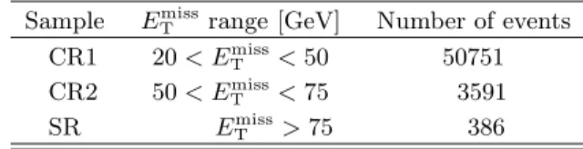
75 GeV, are used to validate the analysis technique and background modeling. Since the control regions should be dominated by background, their data distributions are expected to be well described by the background-only fit. Table V summarizes the number of selected events in CR1 and CR2, as well as those in the signal region (SR), showing that the control region datasets are much larger than that of the signal region. It is of interest whether the background modeling, including the assigned systematic uncertainties, is adequate to describe the control region data within the statistical uncertainties of the data in the signal region. Therefore, the fitting procedure was applied separately to the measured data distributions in CR1 and CR2, scaled in each case to the total of 386 events of the signal region. The fit results for both control regions are in good agreement with the background-only model for all tested signal points, validating the analysis methodology.
TABLE V. Numbers of selected events in the two control re-gions (CR1 and CR2) and in the signal region (SR).
Sample Emiss
T range [GeV] Number of events
CR1 20 < Emiss T < 50 50751 CR2 50 < Emiss T < 75 3591 SR Emiss T > 75 386
Figure 4 shows the distributions of ∆zγ and tγ for the
386 events in the signal region. The distributions of both variables are rather narrow, as expected for background. In particular, there is no evidence for events in the tail
of the tγ distribution at positive times, as would be
ex-pected for a signal contribution due to delayed photons.
The ∆zγ distribution is quite symmetric around zero, as
expected for both the signal and for physics backgrounds.
The |∆zγ| and tγ distributions in the final, coarser
bin-ning are used as inputs to the final fitting procedure and statistical analysis.
Example results of fits to the signal region data are shown in Fig. 5, for the particular case of Λ = 100 TeV and τ = 19 ns. The figures show the results of the signal-plus-background (with µ = 1) and background-only (µ =
0) fits to the six |∆zγ| categories. The signal-region data
are in good agreement with the background-only model, and there is no evidence for a signal-like excess.
Fits to the data were performed for τ values exceed-ing 250 ps, and for the range of relevant Λ values. The
smallest p0 value of 0.21, corresponding to an equivalent
Gaussian significance of 0.81σ, was found for signal model parameters of Λ = 100 TeV and τ = 0.25 ns. Using ensembles of background-only pseudo-experiments, the
[mm] γ z ∆ -2000 -1500 -1000 -500 0 500 1000 1500 2000 Entries/40 mm -1 10 1 10 2 10 > 75 GeV miss T Data E < 20 GeV miss T Data E
ATLAS
= 8 TeV s -1 L dt = 20.3 fb∫
[ns] γ t -4 -3 -2 -1 0 1 2 3 4 Entries/200 ps 1 10 2 10 > 75 GeV miss T Data E < 20 GeV miss T Data E = 0.25 ns τ = 160TeV Λ = 1 ns τ = 160TeV ΛATLAS
= 8 TeV s -1 L dt = 20.3 fb∫
FIG. 4. Distributions of (left) ∆zγ and (right) tγ for the 386 events in the signal region, defined with E miss
T > 75 GeV.
Superimposed are the data distributions for diphoton events with Emiss
T < 20 GeV, used to model the backgrounds, and the
distributions for two example NLSP lifetime values in GMSB SPS8 models with Λ = 160 TeV. The background and MC signal distributions are scaled to the total number of data events in the signal region.
bin γ t 1 2 3 4 5 6 Events/bin -3 10 -2 10 -1 10 1 10 2 10 3 10 4 10 5 10 ATLAS -1 Ldt = 20.3 fb ∫ = 8 TeV: s | < 50 mm γ z ∆ | Signal: =100 TeV Λ )=19 ns 0 1 χ∼ ( τ Data Bkg. Fit =1 Sig. + Bkg. Fit µ bin γ t 1 2 3 4 5 6 Events/bin -3 10 -2 10 -1 10 1 10 2 10 3 10 4 10 ATLAS -1 Ldt = 20.3 fb ∫ = 8 TeV: s | < 100 mm γ z ∆ 50 mm < | Signal: =100 TeV Λ )=19 ns 0 1 χ∼ ( τ Data Bkg. Fit =1 Sig. + Bkg. Fit µ bin γ t 1 2 3 4 5 6 Events/bin -3 10 -2 10 -1 10 1 10 2 10 3 10 ATLAS -1 Ldt = 20.3 fb ∫ = 8 TeV: s | < 150 mm γ z ∆ 100 mm < | Signal: =100 TeV Λ )=19 ns 0 1 χ∼ ( τ Data Bkg. Fit =1 Sig. + Bkg. Fit µ bin γ t 1 2 3 4 5 6 Events/bin -3 10 -2 10 -1 10 1 10 2 10 3 10 ATLAS -1 Ldt = 20.3 fb ∫ = 8 TeV: s | < 200 mm γ z ∆ 150 mm < | Signal: =100 TeV Λ )=19 ns 0 1 χ∼ ( τ Data Bkg. Fit =1 Sig. + Bkg. Fit µ bin γ t 1 2 3 4 5 6 Events/bin -4 10 -3 10 -2 10 -1 10 1 10 2 10 3 10 ATLAS -1 Ldt = 20.3 fb ∫ = 8 TeV: s | < 250 mm γ z ∆ 200 mm < | Signal: =100 TeV Λ )=19 ns 0 1 χ∼ ( τ Data Bkg. Fit =1 Sig. + Bkg. Fit µ bin γ t 1 2 3 4 5 6 Events/bin -3 10 -2 10 -1 10 1 10 2 10 3 10 ATLAS -1 Ldt = 20.3 fb ∫ = 8 TeV: s | < 2000 mm γ z ∆ 250 mm < | Signal: =100 TeV Λ )=19 ns 0 1 χ∼ ( τ Data Bkg. Fit =1 Sig. + Bkg. Fit µ
FIG. 5. Example fit to the signal-region data. The figures show the results of the signal-plus-background fits with µ = 1 to the six |∆zγ| categories, along with the background-only fit and the ±1σ systematic shape variations (dashed lines). The signal
from any one of the 640 signal points in the Λ–τ plane was calculated to be 88%.
Figure 6 shows, for Λ = 200 TeV, the results of the signal-region fit interpreted as 95% confidence level (CL) limits on the number of signal events, as well as on the
signal cross section, as a function of ˜χ01lifetime (assuming
the branching fraction BR( ˜χ01→ γ ˜G) = 1). Each plot
in-cludes a curve indicating the GMSB SPS8 theory predic-tion for Λ = 200 TeV. The intersecpredic-tions where the limits cross the theory prediction show that, for Λ = 200 TeV, values of τ in the range between approximately 0.3 ns and 20 ns are excluded at 95% CL. The observed limits are in good agreement with the expected limits, which are also shown in Fig. 6, along with their ±1σ and ±2σ uncer-tainty bands. For large τ values, the 95% CL limits are close to the value of three events expected for a Poisson distribution with zero events observed, indicating that the results for high lifetimes are dominated by statistical uncertainties. The limits on the number of signal events are higher for low lifetimes, as it becomes more difficult to distinguish between the signal and background shapes. By repeating the statistical procedure for various Λ and τ values, the limits are determined as a function of these GMSB SPS8 model parameters. The range of
˜
χ0
1 lifetimes tested is restricted to τ > 250 ps to avoid
the region of very low lifetimes where the shapes of the signal and background distributions become very simi-lar. Figure 7 shows the subsequent limits in the
two-dimensional GMSB signal space of ˜χ0
1 lifetime versus Λ,
and also versus the corresponding ˜χ0
1 and ˜χ
±
1 masses in
the GMSB SPS8 model. For example, ˜χ01 lifetimes up to
about 100 ns are excluded at 95% CL for Λ values in the range of about 80–100 TeV, as are Λ values up to about
300 TeV (corresponding to ˜χ01 and ˜χ
±
1 masses of about
440 GeV and 840 GeV, respectively) for ˜χ01 lifetimes in
the range of about 2–3 ns. For comparison, the results from the ATLAS analysis of the 7 TeV dataset [1] are also shown in Fig. 7, indicating the significantly larger reach of the 8 TeV analysis.
) [ns] 0 1 χ∼ ( τ 1 10 102
95% CL limit on accepted signal events 1 10 2 10 3 10 Obs. Limit Exp. Limit exp σ 1 ± Exp. Limit exp σ 2 ± Exp. Limit SUSY theory σ ± SPS8 Theory ATLAS -1 Ldt = 20.3 fb
∫
= 8 TeV: s = 200 TeV Λ ) [ns] 0 1 χ∼ ( τ 1 10 102 [fb] σ 95% CL limit on 1 10 2 10 Obs. Limit Exp. Limit exp σ 1 ± Exp. Limit exp σ 2 ± Exp. Limit SUSY theory σ ± SPS8 Theory ATLAS -1 Ldt = 20.3 fb∫
= 8 TeV: s = 200 TeV ΛFIG. 6. The observed and expected 95% CL limits on (left) the number of signal events and (right) the GMSB SPS8 signal cross section, as a function of ˜χ0
1 lifetime, for the case of Λ = 200 TeV. The regions above the limit curves are excluded at 95%
CL. The red bands show the GMSB SPS8 theory prediction, including its theoretical uncertainty.
[TeV]
Λ
100
150
200
250
300
Observed Limit SUSY theory σ 1 ± Observed Limit Expected Limit exp σ 1 ± Expected Limit exp σ 2 ± Expected Limit= 7 TeV Observed Limit s
= 7 TeV Expected Limit s
ATLAS
-1 Ldt = 20.3 fb∫
= 8 TeV: s GMSB SPS8) [ns]
0 1 χ∼(
τ
-110
1
10
210
) [GeV]
0 1 χ∼m(
150
200
250
300
350
400
450
) [GeV]
± 1 χ∼m(
300
400
500
600
700
800
FIG. 7. The observed and expected 95% CL limits in the two-dimensional GMSB signal space of ˜χ01 lifetime versus Λ, the
effective scale of SUSY breaking, and also versus the corresponding ˜χ01 and ˜χ ±
1 masses in the SPS8 model. For comparison,
the results from the 7 TeV analysis are also shown. The regions to the left of the limit curves are excluded at 95% CL. The horizontal dashed line indicates the lowest lifetime value, namely τ = 250 ps, for which the analysis is applied.