HAL Id: hal-00920400
https://hal.archives-ouvertes.fr/hal-00920400
Preprint submitted on 18 Dec 2013
HAL is a multi-disciplinary open access
archive for the deposit and dissemination of
sci-entific research documents, whether they are
pub-lished or not. The documents may come from
teaching and research institutions in France or
abroad, or from public or private research centers.
L’archive ouverte pluridisciplinaire HAL, est
destinée au dépôt et à la diffusion de documents
scientifiques de niveau recherche, publiés ou non,
émanant des établissements d’enseignement et de
recherche français ou étrangers, des laboratoires
publics ou privés.
Branch and Price for a Reliability Oriented DARP
Model
Alain Quilliot, Samuel Deleplanque, Bernay Benoit
To cite this version:
Alain Quilliot, Samuel Deleplanque, Bernay Benoit. Branch and Price for a Reliability Oriented
DARP Model. 2013. �hal-00920400�
adfa, p. 1, 2011.
© Springer-Verlag Berlin Heidelberg 2011
Abstract— We deal here with a static decisional model related to the monitoring of a DARP (Dial and Ride) model which involves, on a closed industrial site, small electrical autonomous vehicles. Because of technological issues, we focus on reliability, and propose a model which assign requests to vehicles while minimizing Load/Unload transactions. We study this model through both a Branch/Price approach, which provides us with bench-marks, and insertion based heuristics, well-fitted to dynamic contexts.
Keywords: Branch and Price, DARP, Reliability, vehicle scheduling
1
Introduction
Current trend in mobility management is to the emergence of flexible reactive sys-tems, which meet mobility demands in a dynamic way while implementing some vehicle sharing and while interacting, through advanced I.T technologies, with alterna-tive transportation modes [16]: Dial and Ride systems, Car-Sharing and Car-Pooling
systems (AUTOLIB…), Ride Sharing systems. Also, recent advances in artificial
perception and remote control make now arise new generations of autonomous (without any driver) individual or collective electrical vehicles: Cycab, VIPA (Individual
Auton-omous Vehicles of LIGIER S.A)…[14], which are involved into the design of those new
mobility services [10]. For this kind of systems, what matters is reliability, related to the steady flow of the traffic induced by the involved vehicle fleet: monitoring has to smooth, as much as possible, the trajectories of the vehicles and minimize orders which require complex interactions between the vehicles.
The model which we handle here, which may be viewed as an extension of interval graph coloring models, is typical of this new kind of problems. It derives from a case study about the management of a specific Dial and Ride system, which involves VIPA automated vehicles and works in real time as a “horizontal elevator”. Constraints are the classical DARP constraints, but performance criterion focuses on Stop
Minimiza-tion: we do in such a way that, as often as possible, vehicles follow their way while
avoiding any break (deviation toward a parking place, load/unload transaction,…) in their trajectory. Though the practical problem has to be handled according to a dynamic
Alain QUILLIOT
Université Blaise Pascal LIMOS CNRS Laboratory,
LABEX IMOBS3 Clermont-Ferrand 63000, France
Email: [email protected]
Samuel DELEPLANQUE
Université Blaise Pascal LIMOS CNRS Laboratory
LABEX IMOBS3 Clermont-Ferrand 63000, France
Email: [email protected]
Benoit BERNAY
Université Blaise Pascal LIMOS CNRS Laboratory,
LABEX IMOBS3 Clermont-Ferrand 63000, France
Email: [email protected]
(on line) point of view, with performance evaluated through discrete event simulation, we consider here, in order to get benchmarks together with a better understanding of the problem, the related static (off line) ILP Stop Minimization decision model. We first deal with this model through a Branch/Price method (Section III). and experimentally check (Section V), that optimizing reliability gets close here to vehicle minimization as well as to global riding time minimization. Next we propose and test (sections IV and V) a greedy randomized insertion heuristic, specially well-fitted to on line contexts.
2
A Static Model
Automated VIPA Vehicles [10], run here along a closed circuit , while meeting
Di-al and Ride demands (see [1, 3, 4, 5]). The nodes are denoted by {0..n = 0}, and the
vehicles always run in the same direction: if a demand is about the transportation of some load L from an origin o to some destination d, then the trajectory of the vehicle which meets this demand is {o, o+1 Mod n, o+2 Mod n,..,d). Circuit is made of a
common track and of load/unload areas, according to figure 1 below:
Figure 1
Node 0 is a Depot node, and the speed of the vehicles on the common track is con-stant (about 15 km/h): thus overtaking is forbidden on the main track, and, when a vehicle gets out some load/unload area, it has no priority on the other vehicles. Vehi-cles meet users on load/unload areas. Running along the whole circuit takes few minutes: so a vehicle which services a given user may run laps around before effec-tively servicing this user. Still we forbid such a user to stay a full tour inside the vehi-cle. Managing the vehicle fleet means, for every demand j, accepting it or rejecting it, and, in case it is accepted, assigning it both a vehicle k and a waiting time h, that is the number of laps the vehicle is going to run before servicing j.
We adopt here a static point of view, and suppose that we are provided with K identical vehicles with capacity C, all located at time 0 in the Depot node. Thus, a
demand j = (o(j), d(j), L(j)) is defined by an origin o(j) and a destination d(j), both in
{0..n}, together with a load L(j). Users ask for the system only when they are ready to move and demands do not involve time-windows. We denote by H the largest waiting
time which is allowed. We suppose that K is large enough to avoid demand rejection.
Since we are concerned here with reliability, which is correlated to load/unload trans-actions, the Stop-Number Problem consists in assigning vehicles and waiting times to
users in such a way that vehicles minimize their Stop Number, i.e. stay as often as possible on the main track without moving onto the load/unload areas.
If we refer to standard Dial and Ride (see [3, 5, 7]), we see that individual riding
times are almost fixed. Still, global riding time and individual waiting times (see [3,
5]) remain part of the problem. As experiments will show, minimizing the Stop
Num-ber also tends to minimize the Vehicle NumNum-ber K as well as the global riding time.
An ILP Model: In order provide our problem with a formal framework, we unfold
the circuit as a linear ordered set I() = {0..(H + 2).n}, which we call the Stop Node
Set. Let DEM = {j = 1..m} be the set of all demands j= (o(j), d(j), L(j)), j = 1..m. In case d(j) < o(j), we replace d(j) by d(j) + n. By proceeding this way, we become able to associate, with every demand j = 1..m, a collection of H + 1 discrete intervals Ij,h =
{o(j) + h.n, …, d(j) + h.n}, h = 0..H, of the Stop Node Set. Clearly, we may suppose
that every node i = 1..n-1 is active, that means such that there exists at least one value j such that i = o(j) or i = d(j). Then, for any node i I() i ≠ (H+2).n, we set:
- A(i) = {(j,h), j = 1..m, h = 0..H, such that o(j) + h.n ≤ i < i+1 ≤ d(j) + h.n}: if a
vehicle k services j A(i) after running h times around , that means according to
waiting time h, then k must be carrying load L(j) when moving from i to i+1;
- B(i) = {(j,h), j = 1..m, h = 0..H, such that (d(j)+ h.n = i) OR (o(j)+ h.n = i)}: if a
vehicle k services j A(i) according to waiting time h then k stops at i.
Then, if the number K of available vehicles is fixed, we get the following ILP model:
Stop-Number(K) ILP Model:
{Compute:
o Z = (Zj,k,h, j = 1..m, k = 1..K, h = 0..H) with {0, 1} values : Zj,k,s = 1 if
vehi-cle k services demand j according to waiting time h;
o T = (Tk,i, k = 1..K, i = 1..n.(H+2)-1), with {0, 1} values : Tk,i= 1 if i is a
stop node for vehicle k. Constraints :
o For any j = 1..m, k,h Zj,k,h = 1; (*Dj is serviced*)
o For any vehicle k, any node i = 0..(H+2).n - 1, (j,h) A(i) L(j). Zj,k,h ≤ C,
(*Capacity Constraints*)
o For any vehicle k, any stop node i = 0..(H+2).n - 1, any (j, h) B(i):
Zj,k,h ≤ Tk,i. (*Coupling Constraints*).
Minimize : k, i Tk,i}
Let V-Stop-Number(K) be the optimal value of Stop-Number(K). Then we get the
Stop Number model: {Compute K which minimizes V-Stop-Number(K)}
Stop Number and Graph Coloring, Remarks about Complexity: If H = 0 and C
= 1, any feasible solution (Z, T) of the Stop-Number problem defines a vertex color-ing of the intersection graph induced by the collection Ij,0 of discrete intervals of the
Stop Node set. Still, though interval graph coloring is known to be time-polynomial
[17], we conjecture that even in this case, the Stop-Number problem is NP-Hard. If H = 0, and no hypothesis is done about C and the loads L(j), j = 1..m, we check that Stop-Number is NP-Hard, since, if K = 2, and o(j) = 0 and d(j) = n-1 for every j = 1..m, then we see that Stop-Number(K) contains the 2-Partition Problem.
If K and C are fixed, and the number H is part of the problem, then Stop-Number may be solved in polynomial time through dynamic programming. It can be checked by following the guidelines of the proof of Proposition 2, Section III.
Extensions and Variants: Introducing time windows in the Stop-Number model,
means setting lower and upper bound Min(j), Max(j), j= 1..m on h(j) values means imposing: Zj,k,h = 0 for any h {Min(j), .., Max(j)}. Also, since we also want to
commpare the Stop-Number criterion with some standard criteria, we provide here variants of the above Stop-Number model, which allow dealing with those criteria:
Vehicle-Number Minimization: {Compute the smallest value K = KMin such that
Stop-Number(K) has a feasible solution}
Global-Riding Minimization: {Compute K = KGlob such that Stop-Number(K) has
a feasible solution and such that the quantity k Ridek is minimal, where Ridek is an
additional integral variable, submitted to the contraints: for any h,j, h.Zj,k,h≤ Ridek} Waiting-Times Minimization: {Compute K = KWait such that Stop-Number(K) has
a feasible solution and such that the quantity j k,h h.Zj,k,h = is the minimal}. Remark: The waiting times criterion is antagonistic to the vehicle number one: KWait
will be such that h(j) = 0 for any j = 1..m.
3
A Branch/Price Method for Stop-Number.
The Stop-Number(K) ILP model is difficult to handle as soon as parameters n, m, H and K do not take small values. Worse, as it also happens for Graph Coloring: [6, 8, 12], above Stop-Number model is not a true ILP one. So, following [1, 9], we re-formulate it as a column generation oriented ILP model. A feasible service is any pair s = (J, h), where J {1..m}, and h some function from {1..m} to {0..H}, such that, for any i = 0..(H+2).n - 1, j D such that (j,h(j)) A(i)L(j) ≤ C. Clearly, a feasible service
iden-tifies the demands j which are serviced by a same vehicle as well as related waiting
times h(j). We denote by S the set of all feasible services. For any s = (J, h) S, we
set Stop(s) = {i 1..(2+H).n – 1, such that B(i) {j, h(j), j = 1..m) ≠ Nil}, and
N-Stop(s) = Card(N-Stop(s)). Then we reformulate Stop-Number problem as follows:
Stop-Number Reformulation:
{Compute: (Xs, s S) with {0, 1} values: Xs = 1 if some vehicle performs the
fea-sible service s.
Minimize : s N-Stop(s).Xs}
Then we may also rewrite the Vehicle-Number problem: {Compute K = minimal number of vehicles and (Xs, s S) with {0, 1} values such that:
- For any j 1..m, s such that j s Xs = 1 ; (*Every demand is serviced once*)
- s Xs≤ K; (*Vehicle number no more than K *)}
By the same way, we notice that, with any service s = (J, h) we may associate: - its Waiting Number N-Wait(s) = j J h(j)
- Its Global Ride Number N-Glob(s) = Sup j J h(j)
So, we may also rewrite the Global-Riding and Waiting-Times variants by replac-ing, inside the Stop-Number reformulation, the “Minimize : s N-Stop(s).Xs“ criterion
by, respectively, “Minimize : s N-Glob(s).Xs” and “Minimize : s N-Wait(s).Xs”.
Methods for the Stop-Number Problem will also work for those problems.
We are now going to describe the Branch/Price procedure, close to clustering algo-rithms of [1] and [13], which will be implemented with the help of the SCIIP library ([14]). In order to do it, we first specify the way tree search, bounding, branching, and constraint propagation are performed. Next we shall address the Pricing issue.
Tree Search: A node N in the search tree induced by the Stop-Number process will
be defined by a collection of additional constraints EX(j1, j2), IN(j1, j2), WAIT+(j, h),
WAIT-(j, h), whose meaning comes as follows: (E1)
- EX(j1, j2) : demands j1, j2 are handled by the same vehicle;
- IN(j1, j2) : j1 and j2 cannot belong to the same service s;
- WAIT+(j, h) (WAIT-(j, h)): the waiting time of j must not be smaller (larger) than h; WAIT constraints restrict the set H(j) of possible h(j) values.
Lower Bound/Branching: We insert (E1) into the Stop-Number ILP by setting:
- In case of a EX(j1, j2) constraint: Xs = 0 for any s containing both j1 and j2; (E2)
- In case of a IN(j1, j2) constraint: Xs = 0 for any s which contains j1 and not j2, and
for any s which contains j2 and not j1; (E3)
- In case of a WAIT+(j, h) (WAIT-(j, h)) constraint: Xs = 0 for any s which contains j
with a waiting time less (more) than h; (E4, E5)
Let us denote by Stop-Number-Aux(EX, IN, WAIT) the resulting ILP. The optimal value of its integral relaxation Stop-Number-Aux(EX, IN, WAIT)* provides us with a
lower bound for
N
. X being some related solution, we get, as in [13]:Proposition 1. If X is not integral, then there must:
- either exist j1 and j2 in {1..m} such that: (E6)
there exist s, such that X ≠ 0 and not integral, which contains both j1 and j2;
there exist s’, such that X ≠ 0 and not integral, which contains j1 and not j2;
- or j, s1 and s2 such that: (E7)
the waiting times h1(j) and h2(j) of j in s1 and s2 are different.
Proof: as in [13]: for any pair (j1, j2), j1 ≠ j2, such that there is no constraint EX(j1,
j2), we denote by (j1, j2) the sum (j1, j2) = j1, j2 s Xs. In case some value (j1, j2) is
non integral, we are done. Else, the pairs (j1, j2) such that (j1, j2) = 1 define a non
oriented graph whose connected components are complete sub-graphs and induce a partition D1.. DP of the set {1..m}. If any j Dp always appear in related services
with the same waiting times, then only one service s = s(p) such that Xs≠ 0 may be
considered as associated with Dp, and X is a feasible integral solution of
Stop-Number-Aux(EX, IN, WAIT). Else we get the (E7) pattern. END-PROOF.
Then we pick up (j1, j2) which satisfies (E6) and branch between EX(j1, j2) and
IN(j1, j2), and, in case of failure, pick up j, s1 and s2 such that (E7) holds, and such that
h1(j) < h2(j), and branch between WAIT-(j, h2(j)) and WAIT+(j, h). In case (E6)
pat-tern may be used, we choose j1, j2, in such a way the sum of their degrees in the union
of IN and EX graphs is the largest possible (most constrained variable principle). In case only (E7) may be used, we choose j which maximizes area (L(j).(d(j) – o(j)).
Constraint Propagation: Given a node N of the Search Tree induced by the
Stop-Number process. We derive constraint propagation inference rules by noticing that:
any connected component of the IN graph should define a complete sub-graph; the EX relation should be extended to those connected components; if G1 is some
con-nected component of the IN graph and if no insertion of j into G1 is possible without
violating either the WAIT constraints or the Capacity constraint, then we should have EX(j1, G1); if only 1 value h exists in H(j), then h(j) should be equal to h.
A. Handling the integral relaxation of Stop-Number-Aux(EX, IN, WAIT).
We do it through column generation. Given S0 S, the restriction
Stop-Number-Aux(EX, IN, WAIT)S0 to S0 of the integral relaxation of Stop-Number-Aux(EX, IN,
WAIT)and ( = (j, j = 1..m)) a related dual solution. Then, Pricing comes as follows: ILP Stop-Number-Price Model:
{Compute:
o Z = (Zj,h, j = 1..m, h = 0..H) with {0, 1} values : Zj,h = 1 if (j, h) is in s ;
o T = (Ti i = 1..(2+H)n-1, with {0, 1} values : Ti = 1 if i Stop(s).
Constraints :
o i = 0..(2+H).n-1: (j, h) A(i) L(j). Zj,h≤ C;
o j =1..m, h = 0..H Zj,h≤ 1; (*No Redundancy Constraint*)
o i = 1..(2+H).n-1, (j ,h) in B(i): Zj,h ≤ Ti; (*Coupling Constraints*)
o (j1, j2) in EX, Zj1 + Zj2≤ 1 ;
(j1, j2) in IN, Zj1 = Zj2 ;Maximize : jj .Zj,h - i Ti, which should > 0}.
We conjecture that this problem is NP-Complete. Still, we may notice that:
Proposition 2: If C is fixed, then Stop-Number-Price is time-polynomial.
Proof. It can be solved as a largest path problem set on an acyclic digraph F with a
number of vertices which depends in a polynomial way on n and H. We first define a
state as being any integer valued vector V = (V1,..,VC), such that n ≥ V1 ≥ V2 ≥ ..≥ VC
≥ -1: the vehicle is loaded with L ≥ c when arriving to any i1 such that i1 ≤ i + Vc and
this L is less than c when the vehicle leaves node i + Vc; V1 = -1 means that the
vehi-cle is empty when it arrives to i. Clearly, V tells us whether the vehivehi-cle unloads or loads at i, and, so, whether i is currently a stop node for s. We denote by SV the set of all possible states. Then nodes in the digraph F are 3-uples (i ,j, V), i I(), j = 1..m, such that o(j) = i modulo n, V SV, augmented with fictitious nodes Start and End. An arc ((i0, j0, V0), (i1, j1, V1)) exists in F if one of the following conditions holds:
- i1 = i0 + 1, j1 = (smallest value j, such that o(j) = i1 modulo n), V1 = V0– 1;
- i1 = i0, j1 = (smallest value j > j0, such that o(j) = i1 modulo n), V1 = V0;
- i1 = i0, j1 = (smallest value j > j0, such that o(j) = i1 modulo n), V1 derives from
V0 by adding load L(j0) between i0 and i0 + d(j0) – o(j0).
In the first 2 cases, the arc ((i0, j0, V0), (i1, j1, V1)) has a null length. In the third
case, it is provided with a length which expresses the impact on the Stop Number of the insertion of j0 into s, taking into account current state V0. One easily checks that
solving Stop-Number-Price means computing a largest path in F. END-PROOF. Still, proposition 2 is hardly suitable for application, since Card(SV) increases as nC. So, in order to deal with the Stop-Number-Price issue in an efficient way, we adopt a double trigger approach: we first try a fast GRASP insertion/removal process, and, in case of failure, we try an exact method involving a flow reformulation.
The Initialization of the GRASP process works by successive insertions of con-nected components G of the IN graph into a current feasible service s, until j sj -
N-Stop(s)) > 0 or no additional insertion is possible, while considering that the largest
are j and Card(H(j)), and the smallest are L(j), d(j) – o(j) and the number of induced
additional stop nodes, the most relevant is inserting j into s; its Local Search loop works as a descent process involving operators Remove(G): demands j G are re-moved from s; Insert(G): demands j G, are inserted into s; Exchange(G1, G2):
per-forms Remove(G1) and next Insert(G2); Move(j, h): the waiting time of j s demand j
is re-assigned to h, where G, G1 and G2 are connected components of the IN graph.
B. Handling Stop-Number-Price through a Max Flow and Lagrangean Relaxation.
Let us introduce the Demand Network D-NET, whose node set is the set {0..(2+H).n-1} and whose arcs are:
o demand arcs aj,h = (o(j)+h, d(j)+h), j =1..m, h = 0..H, provided with a null
low-er capacity Min(aj), an upper capacity Max(aj) = L(j), and a cost Q(aj) = j;
o chain arcs ei = (i, i+1), i = 0..(2+H).n-2; Min(ei) = 0, Max(ei) = + , Q(ei) = 0;
o a backward arc bk = ((2+H).n-1, 0); Min(bk) = Max(bk) = C, Q(bk) = 0.
This allows us to reformulate Stop-Number-Price as the following flow problem:
Flow Stop-Number-Price Formulation.
{Compute on the network D-NET an integral flow vector F, together with 2 {0, 1}-valued vector T = (Ti, i = 1..(2+H).n -1) and U = (Uj, j = 1..m), such that:
o F is consistent with Min/Max capacities ; (E8)
o For any demand arc aj,h, Faj,h = 0 or L(j) ; (E9: Non Load Preemption)
o For any h in {0..m} - H(j), Faj,h = 0; (E10)
o For any j = 1..m, L(j).Uj = h Faj,h; (E11: No Redundancy)
o For any pair (j1, j2) EX: Uj1 + Uj2≤ 1; (E12)
o For any pair (j1, j2) IN: Uj1– Uj2 = 0 ; (E13)
o For any i = 1..(2+H)n -1, j B(i): Uj≤ Ti; (E14)
o Maximize j,hj.Fj,h– 1.T, which should be > 0}.
We relax (E9) and consider the Lagrangean relaxation of (E11). Given multipliers
= (j, j= 1..m) we set: L(F, T, U, ) = .F – 1.T - jj.(L(j).Uj - h Faj,h).
Maxim-izing L(F, T, U, ) may be done by solving 2 independent sub-problems:
- A Max Flow problem about F: {Compute an integral flow vector F, consistent
with capacity and (E10) constraints, and maximizing: j,h (j + j). Faj,h}.
- A problem P-Aux about U and T: {Compute T = (Ti, i = 1..(2+H)n -1) and U =
(Uj, j = 1..m), with {0, 1} values, which satisfy (E12, E13, E14) and which
min-imize 1.T + jj.L(j).Uj. If C-IN is the set of connected components of the IN
graph, then we may extend to C-IN the EX exclusion in a natural way, and
re-place U by a C-IN indexed vector U*, subject to: (Reduced-P-Aux)
o c1, c2 C-IN such that EX(c1, c2), U*c1 + U*c2≤ 1; (E15)
o c C-IN, i = 1..(2+H).n – 1, such that B(i) c ≠ Nil, U*c≤ Ti; (E16)
o The quantity1.T + c (jcj.L(j)).U*c is minimal.
We see that (E15) impose U* to define an independent subset of the graph (C-IN, EX) defined on C-IN by the EX relation. This graph usually happens to be a sparse graph, with few edges, whose cliques and odd cycles with no chords may easily be enumerated. So constraints (E15) may be replaced by stronger con-straints, which are usually facets of the Independent Set polytope (see [2, 9, 15]):
o For any clique Q in the graph (C-IN, EX), c Q U*c ≤ 1; (E15-1)
o For any odd cycle with no chord in the graph (C-IN, EX), c U*c ≤
This makes possible, in most cases, solving Reduced-P-Aux, through a simple relaxation of the integrality constraint followed by a simple rounding process.
Proposition 3: The Non Load Preemption Constraint (E9) contains the integrality
constraints on F, U and T. That means that if F, U, T are rational vectors which satisfy (E8..E14) then they are integral.
Proof: left to the reader. END-PROOF.
As a consequence, we handle Stop-Number-Price through Branch and Bound:
- Bounding derives from computing the Lagrangean value Min Max F, T, U satisfy (E8, E10, E15-1, E15-2, E16) L(F, T, U, ). This process yields some triple F, T, U.
- Branching is performed according to a 3 trigger mechanism:
o If F resulting from bounding does not satisfy (E9), then we pick up aj,h such
that Faj,h≠ 0 and Faj,h≠ 0 L(j), and try both Faj,h = 0 and Faj,h = L(j).
o In case F, U satisfy (E9) and j, h, h’ exist such that Faj,h = Faj,h = L(j), then we
pick up j, h such that Faj,h = L(j) and try both Faj,h = 0 and Faj,h = L(j);
o Else we pick up j such that Uj = 1 and h Faj,h = 0, and branch between Uj = 0,
and the h+1 options Faj,h = 1, h = 0..H.
4
An Insertion Method
Since our ultimate goal is the real time VIPA management, we also propose an in-sertion algorithm Stop-Number-Insert: demands are successively inserted into the vehicles. Such an algorithm links in a well-fitted way off line and on line paradigms: when dealing with an on line instances, we insert, in real time, recent demands into the currently working vehicles. Those usually non deterministic algorithms may be cast into Monte-Carlo schemes. We do not detail here the way Stop-Number-Insert works, and restrict ourselves to a brief description of its general structure:
Stop-Number-Insert Algorithmic Scheme:
J <- {1..m}; K; Service(1) <- Nil; (*Service(k), k = 1..K, is the current service of vehicle k; K denotes a Fictitious Vehicle, and K-1 is the Vehicle Number*)
While J ≠ Nil do
Randomly pick up j0 J, according to some priority rules; (I1)
Compute k0 in 1..K, h0 = 0..H, such that the insertion of j0 into Service(k0)
with waiting time value h(j0) = h0 is feasible and its Quality level is the
highest possible; Insert (j0, h0) into Service(k0) and remove j0 from J; (I2)
If k0 = K then increase K by 1;
Since Stop-Number-Insert is non deterministic, it may be cast into the following
Monte-Carlo scheme, which involves a replication parameter R:
For i = 1..R do Apply Stop-Number-Insert;
Keep the best solution (Service, K-1) ever obtained.
Priority Rules (Instruction (I1)) lead to deal with those among the remaining
de-mands which appear to be the most difficult to insert. Quality criteria lead us to choose k0 and h0 in such a way the fewest possible additional stop nodes are created
and current stop nodes may be reused as often as possible.
5
Numerical Tests
We present here tests, which are performed on a LINUX server CentOS 5.4, Quad-ripro Quadcore, 3 Ghz. In order to deal with ILP models, we use the SCIIP free-access software (see [14]), combined with CPLEX12 LP Library, which efficiently implements the branch/cut/price generic framework. Since no test-bed exists for the
Stop-Number problem, we randomly generate instances, whose characteristics are:
- n = number of stop nodes of the circuit; m = number of demands;
- n-act = number of active nodes; w = mean load value;
- C = capacity of the vehicles; t = mean distance between o(j) and d(j), j = 1..m;
- H = maximum authorized waiting time.
For every such an instance, we try the Stop-Number ILP model of Section II, solved by CPLEX12, the column generation oriented reformulation of Stop-Number of Section III, and the Stop-Number-Insert algorithm of Section IV.
While performing this experiment, we want to evaluate the algorithms, and com-pare the Vehicle Number and Global Riding Time values which derive from the
Stop-Number process with their optimal values. So, for every instance, we denote by:
- KMi the optimal Vehicle Number, and Stop0 the related Stop Number;
- StMin the optimal Stop Number, K1, Ride1, the related Vehicle and Global Riding
numbers; CPU is the running time of the Stop-Number program while Col and
Nd are respectively the numbers of columns and nodes generated by the process;
- Ride the optimal Global Riding Time, and KG the related Vehicle Numbers.
- LB the lower bound induced of Section III
- KIns and StopIns the Vehicle and Stop Numbers which are computed by
Stop-Number-Insert: R is the replication number, and CPUIns the related CPU time (s).
We provide here results for a 7 instance set, generated as told above:
Id = Instance n m n-act H w t C
1 10 40 10 0 1 5 6
2 5 40 5 1 1 2.5 6
6 30 120 30 3 3 15 10
7 30 70 28 4 5 15 10
8 40 150 40 2 1 20 6
10 100 100 89 4 5 50 10
Table 1: Description of the instances.
Id K1 StMin CPU Nd Col LB
1 4 26 37 24 352 25 2 4 13 72 9 751 13 4 2 17 3 1 84 17 6 30 120 30 3 3 15 7 6 86 186 14 356 79 8 4 181 954 16 965 178 10 10 146 11986 24 9896 139
Table 2: Behaviour of the Stop-Number Process of Section III.
Id KINS R=1 StopINS R = 1 CPUINS R = 1 KINS R= 20 StopINS R = 20 1 4 29 0.1 4 26 2 4 15 0.1 4 14 4 2 20 0.2 2 18 6 30 120 30 3 3 7 5 94 0.6 6 90 8 4 208 1.0 4 193 10 9 8.2 0.6 10 3.4
Table 3: Behavior of MC-Stop-Number-Insert.
Instance K CPU (s)
1 4 3
2 4 74
4 2 561
6 No Result *
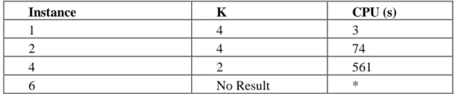
Table 4: CPLEX12 Resolution of the Stop-Number(K) model of Section II
Id KMi Stop0 Ride KG Ride1
1 4 26 0 4 0
2 4 13 3 4 4
4 2 17 2 2 2
6 30 120 30 3 3
8 4 181 7 4 7
10 8 158 30 9 33
Table 5: Feature Analysis.
Comments: The lower bound provided by the linear relaxation of the column
gen-eration oriented reformulation of Stop-Number is very good. Still, running times re-main high, since even when this lower bound happens to be equal to the optimal value of the problem, the linear relaxation of the linear program Stop-Number-Aux may not yield an integral optimal solution. Also, we notice that Stop-Number-Insert, which should efficiently perform in a dynamic context, tends to require fewer vehicles than the exact method, and that optimizing the Vehicle Number also tend to minimize the
Vehicle Number, as well as the Global Riding Time. Finally we may also notice that
unit load instances are easier to handle than instances when the Non Load Preemption
Constraint plays an important role, and, by the same way, that forbidding waiting times, which means assuming H = 0, also tends to make the problem easier to handle.
REFERENCES
[1]. R.BORNDORFER, M.GROTSCHEL, F.KLOSTERMEINER, C.KUTTNER : « Telebus Berlin :
Vehicle routing scheduling in a dial a ride system » ; Konrad Zuse Zentrum Technik Berlin, (1997).
[2]. P.COLL, J.MARENCO, I.DIAZ, I. and P. ZABALA: Facets of the graph coloring polytope, Ann. Operat. Res. (116), p 79-90, (2002).
[3]. J.F.CORDEAU, G. LAPORTE: Dial and Ride : models/algorithms ; An. OR 153-1, p 29-46, (2007). [4]. JF.CORDEAU: A branch and cut algorithm for the Dial/Ride; Oper. Res. 54-3, p 573-586, (2006). [5]. J.F.CORDEAU, M.GENDREAU, G.LAPORTE, J.Y.POTVIN, F.SEMET : « A guide to vehicle routing
heuristics »; Jour. Op. Res. Soc., 53-5, p 512-522, 2002.
[6]. D.CORNAZ, V.JOST: A one to one correspondance between coloring and stable sets, Operat. Res. Letters (36), p 673-676, (2008).
[7]. De PAEPE, K.K.LENSTRA, S.JGALL, R.SITTERS, L.STOUGIE: Computer aided complexity
classi-fication of Dial Ride Problems; INFORMS Journal of Computing 22, p 1130-1152, (2004).
[8]. P.FOUILHOUX: Clique branching formulation for the vertex coloring problem, ISCO Conf. Proc. P 120-124, (2012).
[9]. P.HANSEN, M.LABBE, D.SCHINDL: Set covering and packing formulations of graph coloring:
algorithms and first polyhedral results, Discrete Optimization (6), p 135-147, (2009).
[10]. L.HIGGINS, J.B.LAUGHLIN, K.TURNBULL: Automatic vehicle location and advanced paratransit
scheduling at Houston METROLift; Proc Transport. 2000 Research Board Conf. (2000).
[11]. Y.LUO, P.SCHONFELD: Reinsertion heuristic for DARP; Trans. Res. B 41, p 736-755, (2007). [12]. E.MALAGUTI, M.MONACCI, P.TOTH: An exact approach for the vertex coloring problem, Disc. Optimization, (2010).
[13]. A.MEHROTRA, M.A.TRICK: A column generation approach for grpah coloring, INFORMS Journal of Computing (8), p 344-354, (1996).
[14]. SCIIP: URL http://scip.zib.de.
[15]. I.MENDEZ-DIAZ, P.ZABALA: A cutting plane algorithm for graph coloring, Disc. Applied Math. 154, p 826-847, (2006).
[16]. K. PALMER, M.DESSOUKY, T.ABELMAGUID: Impact of management practices and advanced
technologies on demand responsive transit systems; Transportation Research A 38, p 495-509, (2004).
[17]. C.H.PAPADIMITRIOU, M.YANNANAKIS : « Scheduling interval ordered tasks » ; SIAM Journ. Computing 8, pp 405-409, (1979).
[18]. A.QUILLIOT, S.DELEPLANQUE: Constraint propagation for the Dial and Ride problem wit split