HAL Id: hal-01635450
https://hal.archives-ouvertes.fr/hal-01635450
Submitted on 3 Jun 2020
HAL is a multi-disciplinary open access
archive for the deposit and dissemination of sci-entific research documents, whether they are pub-lished or not. The documents may come from
L’archive ouverte pluridisciplinaire HAL, est destinée au dépôt et à la diffusion de documents scientifiques de niveau recherche, publiés ou non, émanant des établissements d’enseignement et de
Manifold surface reconstruction of an environment from
sparse Structure-from-Motion data
Maxime Lhuillier, Shuda Yu
To cite this version:
Maxime Lhuillier, Shuda Yu. Manifold surface reconstruction of an environment from sparse StructurefromMotion data. Computer Vision and Image Understanding, Elsevier, 2013, 117 (11), pp.1628 -1644. �10.1016/j.cviu.2013.08.002�. �hal-01635450�
Manifold Surface Reconstruction of an Environment
from Sparse Structure-from-Motion Data
Maxime LHUILLIER and Shuda YU
Institut Pascal, UMR 6602, CNRS/UBP/IFMA, Aubi`ere, France
Abstract
The majority of methods for the automatic surface reconstruction of an envi-ronment from an image sequence have two steps: Structure-from-Motion and dense stereo. From the computational standpoint, it would be interesting to avoid dense stereo and to generate a surface directly from the sparse cloud of 3D points and their visibility information provided by Structure-from-Motion. The previous attempts to solve this problem are currently very limited: the surface is non-manifold or has zero genus, the experiments are done on small scenes or objects using a few dozens of images. Our solution does not have these limitations. Furthermore, we experiment with hand-held or helmet-held catadioptric cameras moving in a city and generate 3D models such that the camera trajectory can be longer than one kilometer.
Keywords: 2-Manifold Reconstruction, 3D Delaunay Triangulation, Steiner
Vertices, Complexity Analysis, Sparse Point Cloud, Structure-from-Motion.
1. Introduction
The topic of the paper is the reconstruction of a manifold surface using a sparse method. The definition and the importance of the manifold property are detailed in Sec. 1.1. Sec. 1.2 explains the motivations for a sparse method,
i.e. a method which reconstructs a surface directly from the sparse point
cloud estimated by Structure-from-Motion (SfM). Sec. 1.3 compares our work to the previous sparse methods and Sec. 1.4 summarizes our contributions.
Remember that SfM is a necessary and preliminary step which estimates the successive poses and (sometimes) intrinsic parameters of the camera from an image sequence. The sparsity comes from the fact that the SfM calcula-tions are done for interest points, which have uneven distribucalcula-tions and low
densities in the images (about 1 pixel over 200-300 is reconstructed in our experiments using Harris points [15]).
The sparse methods contrast with the predominant dense methods. There are two main cases of dense methods which estimate a manifold:
1. a surface evolves in 3D such that it minimizes a photo-consistency cost function for all image pixels [11, 17, 18, 31]
2. a surface reconstruction method [41, 6, 21] is applied on a dense point cloud obtained by a dense stereo method [12, 22].
Combinations of both cases are possible (e.g. [23]) and an exhaustive list of references for dense methods is outside the paper scope. By contrast to the dense methods, the sparse methods are less popular and are a minority [10, 19, 27, 29, 32, 36, 38] in the bibliography.
1.1. Why a 2-Manifold ?
In a 2-manifold, i.e. a 2D topological manifold surface, every point of the surface has a surface neighborhood which is homeomorphic to a disk [5]. In short, a 2-manifold is parametrized by two real parameters. In the discrete case, a 2-manifold is usually defined by a list of triangles such that every triangle is exactly connected by its three edges to three other triangles.
The manifold property is required to enforce smoothness constraints on the computed surface. Indeed, the continuous differential operators of normal and curvature are extended to the discrete case thanks to this property [28, 5], and then we can use them to enforce smoothness constraints on the triangle list as in dense stereo [17]. More generally, a lot of Computer Graphic algo-rithms are not applicable if the triangle list is not a 2-manifold [5]. In our work, the manifold property is used to constrain a surface interpolating the sparse SfM point cloud and to improve surface denoising.
1.2. Why a Sparse Method ?
There are several reasons to estimate a surface directly from the sparse SfM cloud. First, it would be ideal for both time and space complexities. This is interesting for obtaining compact models of large and complete envi-ronments like cities or for an implementation in a small embedded hardware. Second, it could be used for navigation pre-visualization [8], for initialization of dense stereo methods (e.g. [17, 18]), or for autonomous navigation [7]. Last, the accuracy of a point in SfM cloud is expected to be better than that of a point in a dense stereo cloud, thanks to the SfM machinery [16] involving interest point detection and bundle adjustment.
(A) (B)
Figure 1: Delaunay-based reconstruction in the 2d case (surfaces, tetrahedra and triangles are replaced by curves, triangles and edges, respectively). (A) curves to be reconstructed and points which sample the curves. (B) the Delaunay triangulation of the points. Note that the inside of [4] is the gray region, but our inside (Sec. 2) is the white region.
1.3. Previous Works
Methods [10, 19, 27, 29, 32, 36, 38] using our input (sparse SfM data) start by establishing potential adjacency relationships between the input points, which are selected latter to build a surface. These methods can be classified by examining the data structures encoding the potential adjacencies: [10, 32, 27, 38] use one 3D Delaunay triangulation (Sec. 1.3.2) and [29, 36, 19] use 2D Delaunay triangulations (Sec. 1.3.3). The SfM data also includes visibility constraints, i.e. line segments (rays) which should not intersect the target surface, except at a segment end. A ray links a point to one of the view points used by SfM to reconstruct the point.
1.3.1. Sculpting in a 3D Delaunay without Rays
The sculpting method in [4] is closely related to our method, although it does not use rays. It partitions R3
into tetrahedra of the 3D Delaunay triangulation of the input points. The tetrahedra are labeled as inside or
outside, and the surface is the list of triangles which bound the inside region
(according to [2] and Fig. 1, a “good” surface can be obtained by such a segmentation). Every tetrahedron is initialized inside; the remainder of R3
is outside. Then an inside tetrahedron is selected by a geometric criterion and becomes outside while the resulting surface is manifold and every Delaunay vertex is in an inside tetrahedron. This method requires that the input point cloud is denser that ours and does not contains bad points.
1.3.2. Sculpting in a 3D Delaunay with Rays
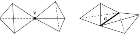
Methods [10, 22, 32, 27, 38, 39] use rays to label the tetrahedra of the 3D Delaunay triangulation: a tetrahedron is freespace if it is intersected by ray(s), otherwise it is matter.
v
e
Figure 2: Surface singularities defined by two freespace tetrahedra in matter space.
In contrast to our method, [22, 32] do not enforce manifold constraint and [27] directly consider the surface as the list of triangles separating the
freespace and matter tetrahedra. Then, the resulting surface can be
non-manifold. For example, the surface has a singularity at vertex v if all tetra-hedra which have vertex v are matter, except two freespace tetratetra-hedra ∆1 and
∆2 such that the intersection of ∆1 and ∆2 is exactly v (left of Fig. 2).
An-other singularity example is obtained if we replace “vertex v” by “edge e” in the previous example (right of Fig. 2). A post-processing [13] can be applied to obtain a 2-manifold by removing the singularities, but such an approach does not enforce the manifold constraint during the surface calculation and generates new vertices for every singular vertex.
Only [10] and our previous work [38, 39] provide a 2-manifold. In [10], a region growing procedure in the matter tetrahedra removes all surface singu-larities and reconstructs very simple scenes. In [38, 39], the region growing is in the freespace tetrahedra and deals with more complex topologies than those in [10, 4]: the estimated surface can be a torus with several handles. Our region growing is essentially a best first approach based on the number of ray intersections per tetrahedron ([10] does not use this information). In [39], artifacts called “spurious handles” and generated by [38] are removed while maintaining the manifold property. Here the largest handles are removed thanks to the tetrahedron labels (e.g. freespace). The previous removal methods [37, 42] remove the smallest handles without these labels.
1.3.3. 2d Delaunay-based Work
Methods [29, 36, 19] use 2D Delaunay triangulations in images. In [19], the surface is not 2-manifold and the approach is applied to a small sequence of real images. In [29], the surface is a 2-manifold limited to a simple topology (sphere or plane). In [36], reconstructed edges are inserted in the constrained 2D triangulations, then the back-projected 2.5d triangulations are merged by computing the union of the freespace defined by the 2.5d triangulations. The resulting implicit surface is converted to manifold mesh by the marching cube method [26], which requires a thin-scale regular subdivision of space.
However, an irregular space subdivision is better for large scale scene [22]. Compared to these methods, ours estimates a 2-manifold without topology limitation and without thin-scale regular space subdivision.
1.4. Paper Contributions
According to Sec. 1.3.2 and 1.3.3, our contributions over the other sparse methods are the following: we combine both 2-manifold and visibility con-straints without limitation on the surface genus (i.e. the number of handles of the surface), and the experiments are done on larger image sequences of com-plete environments (hundreds/thousands of images in a few seconds/minutes). Furthermore, this paper is an extended version of our previous work [38, 39]. New material includes: highlight of our method with visibility optimization (Sec. 2), efficient tetrahedron-based manifold test (Sec. 2), discussion on bad SfM points (Sec. 3.6), complexity analysis (Sec. 5 and 6). Sec. 3 describes the overall method, then artifacts called “spurious handles” are removed by the methods in Sec. 4. Also there are new experiments in Sec. 7 about manifold constraint, varying densities of reconstructed and Steiner points, comparison with the Poisson surface reconstruction [21], larger still and video sequences. Note that we do not focus on the incremental surface reconstruction [40].
2. Prerequisites on 2-Manifolds embedded in a 3D Delaunay Our algorithm needs prerequisites on 2-manifolds embedded in a 3D De-launay triangulation. Here we introduce notations (Sec. 2.1), our optimiza-tion problem (Sec. 2.2), and the 2-manifold tests (Sec. 2.3).
2.1. Notations and Tetrahedron Labeling
Let P be a set of reconstructed points. The 3D Delaunay triangulation of P is a list T of tetrahedra which meets the following conditions: the tetrahedra partition the convex hull of P , their vertex set is P , and the circumscribing sphere of every tetrahedron does not contain a vertex in its interior. A vertex/edge/triangle is a face of a tetrahedron in T . Assuming L ⊆ T , border δL is the list of triangles which are included in exactly one tetrahedron of L. Let F ⊆ T be the list of freespace tetrahedra, i.e. the tetrahedra intersected by ray(s). The tetrahedra which are not freespace are matter. According to Sec. 1.3.2, δF can be non-manifold. Here we introduce O ⊆ F , the list of outside tetrahedra, such that δO is manifold. The tetrahedra which are not outside are inside.
We also consider T as a graph: a graph vertex is a tetrahedron, a graph edge is a triangle between two tetrahedra. A standard practice is to introduce infinite vertex v∞ such that we define a virtual tetrahedron connecting δT
triangle and v∞ [1]. The virtual tetrahedra do not exist in 3D, but they
are vertices of the graph. They make easier both implementation and paper clarity since every tetrahedron has exactly four neighbors in the graph.
Since P is reconstructed in all directions around the view points to model complete environments, all rays are included in the convex hull of P . Then the virtual tetrahedra are labeled matter. Every matter tetrahedron is inside. Note that δF and δO are closed surfaces; δF cutsR3 into free-space (F )
and matter, δO cuts R3
into outside (O) and inside. Furthermore, O ⊆ F .
2.2. Optimization Problem for 2-Manifold Extraction
In short, the target surface δO is a 2-manifold which should separate the
matter and free-space tetrahedra “as much as possible”. Let r : F → R+∗ a
scalar and positive function. We extend r to O ⊆ F by r(O) =P
∆∈Or(∆).
We would like to estimate O included in F and maximizing r(O) subject to the constraint that δO is a 2-manifold. Intuitively (if r = 1), a large O in F with a 2-manifold border δO is a good solution. Now we give two remarks.
First, this optimization problem is difficult due to the manifold constraint. Then we solve it using a greedy algorithm: we add progressively free-space tetrahedra in O as long as δO remains a 2-manifold, then r(O) increases and the final δO is an approximation of the exact solution of our problem.
Second, several definitions of r are possible. Here we optimize visibility by defining r(∆) as the number of rays which intersect tetrahedron ∆. Since our paper focuses on manifold extraction and related complexity, we do not investigate on more sophisticated definitions of r inspired by [27, 32, 22, 20].
2.3. 2-Manifold Tests
Here we explain how to check that a surface S (a list of triangles of T ) is a 2-manifold. This topic is somewhat technical but very important in practice for the computation time of our method.
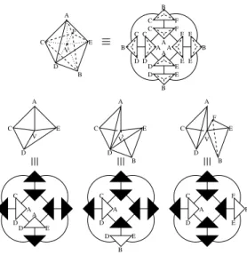
Let v be a point in S. We say that v is regular if it has a neighborhood in S which is topologically a disk. Otherwise v is singular. By definition (Sec. 1.1), S is 2-manifold if all its points are regular. In our context where S is a list of triangles of T , we only need to check that every vertex v of S is regular using the following neighborhood of v: the list of the S triangles which have vertex v [4]. Now we describe three 2-manifold tests.
A C V V V A A C C D D D B B E E E F
Figure 3: Regular and singular vertices. Left: v is regular since the edges opposite to v define a simple polygon acdea on the surface. Middle: v is singular since polygon dacdbedhas multiple vertex d. Right: v is singular since acda− befb is not connected.
2.3.1. Polygon-Based Vertex Test
Vertex v is regular if and only if [4] the edges opposite to v in the triangles of S having v as vertex form a simple polygon (Fig. 3). A simple polygon is topologically a circle, i.e. a list of segments which forms a closed path without self-intersection. This test was used in our previous work [38, 39].
2.3.2. Graph-Based Vertex Test
The test in Sec. 2.3.1 is adequate if the surface S is implemented as an adjacency graph of triangles. This is not the case here since S is embedded in a Delaunay T implemented as an adjacency graph of tetrahedra.
So we introduce a faster test to check that v is regular. Let gv be the
graph of the tetrahedra incident to v (gv is a sub-graph of T ). Appendix A
shows that the v-opposite edges above form a simple polygon if and only if the inside tetrahedra of gv are connected and the outside tetrahedra of gv
are connected (Fig. 4). Thus we check that v is regular thanks to a simple traversal of graph gvwhere the edges between inside and outside are removed. 2.3.3. Incremental Use of the Vertex Tests
Now we explain how to use the 2-manifold tests in Sec. 2.3.1 and 2.3.2. In our context, S = δO is estimated by a greedy method (Sec. 2.2). Assume that δO is a 2-manifold. We add A ⊆ F into O. Then we should check that (the new) δO is still a 2-manifold. We collect in list W all vertices of the tetrahedra in A which are in δO. The new δO is a 2-manifold if every vertex in W is regular. Otherwise, it is not and A is removed from O. The vertices of δO which are not in W do not need to be checked since the labels
outside-inside of their incident tetrahedra do not change by adding A. 2.3.4. Single Tetrahedron Test
In the special case where list A contains a single tetrahedron ∆, there is a test based on [4], which is faster than those in Sec. 2.3.3. In this case, we
A C V V V A A C C D D D B B A A D E D C A C D D E B C A D F E B A B D C E V E E E F F B F C C C C FF F B E E E E D D D D AAA A B B
Figure 4: Relation between topology and graph. Top: 8 tetrahedra incident to v and their adjacency graph gv. Bottom: three cases of tetrahedra labeling (inside is black, outside is
white). Middle: the resulting topology around v. Middle and bottom: v is regular if and only if the inside tetrahedra are connected and the outside tetrahedra are connected.
first check a condition on O and then add ∆ to O (if the condition is meet). This condition is detailed in Appendix B. It only requires to read once the lists of tetrahedra incident to the four ∆-vertices.
3. Surface Reconstruction Algorithm
Every sub-section describes a step of our method, except the last one which discusses bad (false positive) SfM points.
3.1. 3D Delaunay Triangulation T
Assume that SfM estimates the geometry of the whole image sequence. The geometry includes the sparse cloud of points{pi}, camera locations {cj}
and rays defined by visibility lists{Vi}. List Vi is the list of indices of images
which reconstruct the 3D point pi, and a ray is a line segment linking pi to
cj if j ∈ Vi. The size of Vi is greater than 2 (2 is the theoretical minimum
but it is insufficient for robustness).
Point pi has poor accuracy if it is reconstructed in degenerate
configura-tion [16]: if pi and all cj, j ∈ Vi are nearly collinear. This case occurs in part
from this part are close to the straight line. Thus, the point cloud is filtered as in [9]: pi is added in T if and only if there is {j, k} ⊆ Vi such that angle
\
cjpick meets ǫ≤ \cjpick ≤ π − ǫ using threshold ǫ > 0. 3.2. Ray Tracing
We set r = 0 and apply ray tracing to all rays. Since T is a graph (Sec. 2.1), tracing a ray cjpi is a walk in the graph, starting from a
tetra-hedron incident to pi, moving to another tetrahedron through the triangle
intersected by the line segment cjpi, and stopping to the tetrahedron which
contains cj (the inverse walk is also possible). Ray cjpi is traced if and only
if pi is a vertex of T . For every tetrahedron ∆ intersected by a ray, r(∆) is
increased by 1. We obtain function r and list F of the free-space tetrahedra.
3.3. 2-Manifold Extraction
According to Section 2.2, we use a greedy algorithm to approximate the list O which maximizes r(O) such that δO is a 2-manifold and O ⊆ F : O grows from ∅ by adding free-space tetrahedra such that δO remains 2-manifold. The result of this step is the final δO. We use r to define a priority for the free-space tetrahedra: the ∆s with the largest r(∆) are added in O before others. Due to the manifold constraint, we also require that the selected ∆ has (at least) one face in δO to avoid that the greedy algorithm gets stuck too easily in a bad solution
The tetrahedra in the neighborhood of O are stored in a heap (priority queue) for fast selection of the tetrahedron with the greatest r. Thus O usually grows from the most confident free-space tetrahedra (with large r) to the less confident ones (with small r).
Algorithm 1 presents our growing method in C style. The inputs are the initial O, list F , list Q0 of tetrahedra which includes the initial value of the
heap, and function r. Here we use O =∅ and Q0 =∅. The output is O. 3.4. Topology Extension
The outside region O computed in Sec. 3.3 has the ball topology since we add tetrahedra one-by-one [4]. This is problematic if the true outside does not have the ball topology, e.g. if the camera trajectory contains closed loop(s) around building(s). In the simplest case of one loop, the true outside has the toroid topology and the computed outside O can not close the loop (as shown by Fig. 5).
Algorithm 1 Outside Growing
01: Q=∅; // *** initialization of priority queue Q *** 02: if (O==∅) { // Sec. 3.3
03: let ∆∈ F be such that r(∆) is maximum; 04: Q← Q ∪ {∆};
05:} else for each ∆ ∈ Q0∩ F // Sec. 3.4
06: if (∆ /∈ O and ∆ has a 4-neighbor in O) 07: Q← Q ∪ {∆};
08: while (Q!=∅) { // *** region growing of O *** 09: pick from Q the ∆ which has the largest r(∆); 10: if (∆∈ O) continue;
11: O ← O ∪ {∆};
12: if (all vertices of ∆ are regular) {
13: for each 4-neighbor tetrahedron ∆′ of ∆
14: if (∆′ ∈ F and ∆′ ∈ O)/
15: Q← Q ∪ {∆′};
16: } else O ← O \ {∆}; 17:}
Figure 5: Close the loop. Left: adding one tetrahedron (dark) at once in O (light) can not close the loop due to singular vertex. Right: adding several tetrahedra at once can do it.
This problem is corrected as follows. Firstly, we find a vertex in δO such that all inside tetrahedra incident to this vertex are free-space. Secondly, these tetrahedra are collected in list A. Thirdly, we try to add A into O using a 2-manifold test in Sec. 2.3. At last, if the test is successful, we use the region growing in Sec. 3.3 where Q0 is the list of tetrahedra neighbors of
A. In practice, we go through the list of δO vertices several times to do this process.
3.5. Post-Processing
Although the surface S provided by the previous steps is a 2-manifold (S = δO), it has several weaknesses which are easily noticed during visual-ization. Now we examine these weaknesses and explain how to remove or reduce them using prior knowledge of the scene.
3.5.1. Peak Removal
A peak is a vertex pi on S such that the ring of its incident triangles in
S defines a solid angle w which is too small to be physically plausible, i.e. w < w0 where w0 is a threshold. Let L be the list of the tetrahedra in the
acute side of the peak ring. L is outside or inside. Now we reverse the L label: inside becomes outside, and vice versa. The removal of peak pi from S
is successful if all vertices of the L tetrahedra remain regular. Otherwise, the label of L is restored to its original value and we try to remove another peak. In practice, we go through the list of S vertices several times to detect and remove peaks. Note that this step ignores the free-space/matter labeling.
3.5.2. Surface Denoising
The S reconstruction noise is reduced thanks to a smoothing filter p′ =
p+ ∆p where p is a vertex of S and ∆p is a discrete Laplacian defined on S vertices [35]. The smoothed p′ is stored in a distinct array of p. We don’t
apply p← p′ to avoid the computation overhead due to vertex update in T . 3.5.3. Sky Removal
Up to now, S is closed and contains triangles which correspond to the sky (assuming outdoor image sequence). These triangles should be removed since they do not approximate a real surface. They also complicate the visualization of the 3D model from a bird’s-eye view. Firstly, the upward vertical direction u is robustly estimated assuming that the camera motion is (roughly) on a horizontal plane. Secondly, we consider open rectangles
defined by the finite edge cici+1and the two infinite edges (half lines) starting
from ci (or ci+1) with direction u. A triangle of S which is intersected by an
open rectangle is a sky triangle and is removed from S. Now S has hole in the sky. Lastly, the hole is increased by propagating its border from triangle to triangle while the angle between triangle normal (oriented from outside to
inside) and u is less than threshold β. 3.6. Bad (False Positive) SfM Points
SfM can reconstruct bad point p due to repetitive texture or image noise. Now we discuss the consequences and give solutions for this problem. If p is in the true matter of the scene, there are tetrahedra that should be matter which are labeled free-space due to bad ray of p. If these tetrahedra are in O, δO can be corrupted, e.g. a wall with a spurious concavity. In practice, the risk of bad p is low thanks to the SfM machinery (bundle adjustment, RANSAC, robust matching, interest point detectors).
Nevertheless, our method reduces this risk and can remove spurious con-cavities. First, the risk is reduced thanks to the choice of ǫ in the point selection step (Sec. 3.1): the larger ǫ, the more accurate points and their rays used by Ray Tracing (Sec. 3.2), the lower risk of spurious concavity. Second, the spurious concavities created by the manifold constraint in the growing steps (Sec. 3.3 and 3.4) can not be worse (larger) than those of the
free-space in the matter. Indeed, a concavity is a list of outside tetrahedra
which are included in free-space. Third, Appendix C explains how Peak Removal (Sec. 3.5.1) can remove spurious concavities.
4. Removal of Spurious Handles
Sec. 4.1 introduces spurious handles. Then two removal methods are presented in Sec. 4.2 and 4.3, which complete our methods in Sec. 3 (the removal methods are not presented in Sec. 3 for the paper clarity).
4.1. Definition of Spurious Handles
Topology Extension (Sec. 3.4) calculates a 2-manifold without genus con-straint and improves our solution of the optimization problem (Sec. 2.2), but it has one drawback: it can generate spurious handles. Fig. 6 shows an ex-ample in a real case: the oblique handle on the left connects a small wall to the ground. This handle is spurious: it does not exist on the true scene surface and it should be removed while maintaining the manifold property.
Figure 6: Spurious handle (left) and its removal (middle and right).
In the paper, we remove the handles which are both “visually critical” and due to “incomplete” outside growing in the free-space. “Visually critical” means that we ignore the handles that are too small to be easily noticeable by viewers (virtual pedestrians) located at all view points cj reconstructed
by SfM. “Incomplete” means that the handles only contains free-space tetra-hedra that are inside and which should be forced to outside. We use these conditions to localize the spurious handles and to obtain a final 2-manifold which meets the visibility constraints provided by the rays. For the remain-der of the paper, a “spurious handle that is visually critical and due to incomplete growing” is shortened to “spurious handle”.
Our spurious handle removal methods use Steiner vertices, i.e. extra points in T which are not in the original (SfM) input. The Steiner vertices do not have rays.
4.2. Method 1: Reduce Size of Tetrahedra
In [38], a simple method is used to reduce the risk of spurious handles. In the 3D Delaunay step (Sec. 3.1), Steiner points are added in T such that the long tetrahedra potentially involved in spurious handles are split in smaller tetrahedra. The Steiner points are added in the critical region for visualiza-tion: the immediate neighborhood of the camera trajectory. We randomly add a fixed and small number of Steiner vertices at the neighborhood of ev-ery camera location cj. A neighborhood is a ball centered at cj with radius
defined as a multiple (e.g. 10) of meanj||cj+1− cj||. 4.3. Method 2: Detect, Force and Repair
Another removal method [39] is applied after “Topology Extension” and before “Post-Processing”. Every sub-section describes a step of the method.
b a e d c a b c e d f
Figure 7: Spurious handle (left) and Edge Splitting (right) in the 2D case. Bold edges = manifold edges, simple edges= Delaunay edges, white region= outside, light gray= inside-freespace, dark gray= inside-matter. Left: edges ab, cd, ac are visually critical. Right: Steiner point f is inserted on cd, this splits triangle cde and adc.
4.3.1. Detect Visually Critical Edges
Let e be an edge with finite vertices ae and be. Let α > 0 be a threshold.
Edge e is “visually critical” if
1. every tetrahedron including e is free-space and 2. at least one inside tetrahedron includes e and
3. there is a view point cj such that angle \aecjbe is greater than α.
The first step is the calculation of all visually critical edges in list Lα. A
spurious handle has critical edges both on its border and its interior (Fig. 7). The larger α, the smaller size of Lα and also the greater lengths of the
edges in Lα. We use this to select a moderated number of handles and
apply on every selected handle a processing, whose time computation per tetrahedron/vertex is greater than those in Sec. 3.3 and 3.4.
4.3.2. Force Tetrahedra Outside
This step needs a mesh operator called “Edge Splitting”. It splits an edge of T by adding a Steiner vertex on the edge, and every tetrahedron including the edge is also split in two tetrahedra whose labels (free-space,
matter, inside, outside) are the same as the original tetrahedra. Thus, the
resulting triangulation T is not 100% Delaunay after this step, but our surface δO which separates outside and inside tetrahedra is still a 2-manifold (the set of surface points is unchanged).
Now we split every Lαedge by a Steiner vertex on its middle (one example
in Fig. 7). This changes the graph of tetrahedra and provides new tetrahedra for the next step, which is a local region growing of O in F . For each vertex vi
on (split) critical edges, we define the list of tetrahedra Liincident to viwhich
are free-space and inside. Then a first round of (Force,Repair) is applied to the list Li. Function “Force” adds tetrahedra in O without checking that δO
is a 2-manifold, and function “Repair” (Sec. 4.3.3) tries to grow O such that δO becomes a 2-manifold. If it fails, another round of (Force,Repair) is tried for every tetrahedron of Li. Algorithm 2 presents our method in C style.
Algorithm 2 Force Tetrahedra Outside
01: for each vertex vi of the (split) edges of every e ∈ Lα {
02: let Li be the list of tetrahedra incident to vi;
03: G = (Li∩ F ) \ O;
04: O ← O ∪ G; // Force 05: if (!Repair)
06: for each tetrahedron ∆∈ Li
07: if (∆∈ F and ∆ /∈ O) { 08: G ={∆}; 09: O ← O ∪ G; // Force 10: Repair; 11: } 12:}
4.3.3. Repair δO by local growing of O
The repair step is a local growing of O in F such that the number n of sin-gular vertices of surface δO decreases and every resin-gular vertex is maintained regular. At the beginning, n > 0 is due to the addition of G in O (Force). Then a free-space and inside tetrahedron ∆ is chosen in the neighborhood of G, and it is added to O. If n increases, we remove ∆ from O and try another tetrahedron. We continue until every ∆ candidate increases n. If the final n is 0, the local region growing succeeds. Otherwise it fails and O is restored to its value before the Force step.
The inputs are O, G and g0 (an upper bound to limit the local growing
complexity). The output is a boolean which asserts that Repair is successful or failed. Repair can also modify O. Algorithm 3 presents function Repair in C style. Note that this algorithm looks like the one in Sec. 3.3. The main differences are (1) the 2-manifold tests are replaced by non-increase tests of the number of singular vertices and (2) the process can fail.
5. Starting the Complexity Analysis
Here we evaluate the time complexities of the 2-manifold tests (Sec. 5.2) and region growing (Sec. 5.3) using notations and data structures in Sec. 5.1.
Algorithm 3 Repair
01: let Y be the list of vertices of the tetrahedra in G; 02: let n be the number of singular vertices in Y ; 03: // **** initialization of priority queue Q **** 04: Q=∅;
05: for each tetrahedron ∆ in G
06: for each 4-neighbor tetrahedron ∆′ of ∆
07: if(∆′ ∈ F and ∆′ ∈ O)/
08: Q← Q ∪ {∆′};
09: // **** region growing of O **** 10: while (Q!=∅) {
11: pick from Q the ∆ which has the largest r(∆); 12: if (∆∈ O) continue;
13: let b0
i be true iff the i-th vertex of ∆ is singular
14: n0 =P 4 i=1b
0
i; // number of singular ∆-vertices
15: O ← O ∪ {∆}; 16: let b1
i be true iff the i-th vertex of ∆ is singular
17: n1 =
P4
i=1b 1
i; // number of singular ∆-vertices
18: if (n0 ≥ n1 && b01 ≥ b 1 1 && b 0 2 ≥ b 1 2 && b 0 3 ≥ b 1 3 && b 0 4 ≥ b 1 4) { 19: G← G ∪ {∆}; // G is used latter 20: n← n + n1− n0; // fast n update 21: if(the size of G is g0)
22: break; // too large computation: stop 23: for each 4-neighbor tetrahedron ∆′ of ∆
24: if (∆′ ∈ F and ∆′ ∈ O)/
25: Q← Q ∪ {∆′};
26: } else O ← O \ {∆}; // failure of ∆ addition 27:}
28: // **** check the result **** 29: if (n) {
30: O ← O \ G; 31: return 0; 32:} else return 1;
Then Sec. 5.4 discusses the worst case complexities of these steps and others. We use the standard “big o” notation O; x is bounded if x = O(1).
5.1. Notations and Data Structures
The 3D Delaunay triangulation T is the labeled graph defined in Sec. 2.1. We note|L| the number of elements of list L; |T | is the number of tetrahedra. Let v be the number of tetrahedra vertices. We assume that every tetrahe-dron ∆ stores a label outside-inside, the number r(∆) of intersected rays, the list of 4 vertices, and the list of 4 neighbor tetrahedra. The tetrahedra and their vertices are referenced by integers in the lists above. There is a table of vertices and a table of tetrahedra. Note that ∆∈ F if and only if r(∆) > 0. Let d be the maximum vertex degree, i.e. the number of tetrahedra incident to every finite vertex (every vertex except v∞) is less or equal to d.
5.2. Complexity of the 2-Manifold Tests
In Sec. 2.3.3, we add A to O if and only if δO remains 2-manifold, i.e. if every vertex of W is regular. According to Sec. 3.3 and 3.4, A has a single tetrahedron or several tetrahedra sharing a surface vertex. This vertex can not be v∞ since all v∞-incident tetrahedra are matter and every surface
vertex is incident to a free-space tetrahedron. Thus, |A| ≤ d. Since W is the list of the vertices of the tetrahedra in A, its complexity isO(d). Furthermore, the complexity to check that a vertex is regular using the Graph-Based Test in Sec. 2.3.2 is O(d). Thus the time complexity of the 2-manifold test for list A is O(d2
). If A has a single tetrahedron, both graph-based method (Sec. 2.3.2) and single tetrahedron method (Appendix B) are O(d).
5.3. Complexity of One Region Growing
Here we estimate the time complexity of Algorithm 1. Let q0 be the
number of tetrahedra in list Q0. Let g be the number of grown tetrahedra, i.e. the difference between the number of tetrahedra in the output O and
the number of tetrahedra in the input O of this algorithm. A tetrahedron ∆ is definitely added at most one time into O. In this case, at most four tetrahedra are added to Q. There is no other addition to Q, except at the initialization of Q where there are at most O(q0) additions to Q. Thus, the
number of “while” iterations is O(g + q0).
Now the time complexity of one iteration is estimated. Picking the best tetrahedron in heap Q isO(log(g+q0)). The other instructions in one “while”
If we start from O =∅, we should add the complexity of Q initialization: the time complexity of one region growing is O(|T | + g(d + log(g))). If we start from O 6= ∅, this time complexity is O((g + q0)(d + log(g + q0))). 5.4. Loose Results
The number of tetrahedra is|T | = O(v2) and the maximum vertex degree
is d = O(v) since T has v vertices [3, 34]; the worst case exists but it is rare. Furthermore, a theoretical study starting from these numbers provides time complexities that are not tight enough to be interesting. Here are two examples. First, the time complexity in the worst case to trace a single ray is O(v2
). Indeed, one line segment can intersect all tetrahedra [34], but this is almost impossible in practice. A second example is the region growing which is O(v3
) in the worst case (use d = O(v) and g + q0 = O(v2) in Sec. 5.3),
but it is quite smaller in practice. So we will use neither |T | = O(v2
) nor d =O(v) in the complexity analysis below.
6. Tight Time Complexity
Sec. 6.1 introduces two new assumptions: the bounded density of the SfM points and the addition in T of a Cartesian grid of Steiner vertices. Sec. 6.2 lists all our assumptions and Sec. 6.3 provides the worst case time complexities for the steps of our method.
6.1. Additional Point Assumptions and their Consequences
We assume that the density of reconstructed points in 3D is bounded: there are p > 0 and q > 0 such that every p-ball contains at most q points. A p-ball is a ball with radius p. This could be justified as follows: (1) only interest points are reconstructed and (2) the scene surface has texture such that the interest points, which are detected due to grey-level 2D variations in their neighborhood, have a bounded density (e.g. no fractal-like texture). We also use a bounding box of the reconstructed points, which is com-puted from the point coordinates. This box has Delaunay mesh T with two kinds of vertices: the reconstructed vertices (Sec. 3.1) and Steiner vertices located at the corners of a Cartesian grid. The adding of Steiner vertices (i.e. extra points) is a standard method in Computational Geometry to generate meshes with good properties, e.g. to guarantee a linear-size 3D Delaunay triangulation with bounded vertex degree [3]. Every Steiner vertex has an
empty visibility list. In practice, the number s of Steiner vertices is quite smaller than the number m of reconstructed vertices (v = m + s≈ m).
Thanks to the bounded density of the SfM points and the Cartesian grid of Steiner vertices, Appendix D shows that the tetrahedron density is also bounded, i.e. there are p′ > 0 and q′ > 0 such that every p′-ball intersects
at most q′ tetrahedra. The proof has two steps: first the tetrahedron
diam-eter is bounded by the diagonal length l of a grid voxel, second we use the bounded density of the points in the p′+ l-ball which includes all tetrahedra
intersecting the p′-ball. If the p′-ball is centered at a finite vertex, we see
that the maximum vertex degree d is bounded.
6.2. List of Properties and Assumptions
This list is used in the complexity proofs.
H0: T has m reconstructed and s Steiner vertices where s < m H1: the tetrahedron density is bounded
H2: the maximum vertex degree d is bounded
H3: the access to the 4 neighbors of a tetrahedron is O(1) H4: the size of visibility list Vi is bounded
H5: the distance between two consecutive view points is bounded.
H0-2 are in Sec. 6.1. H3 is in Sec. 5.1. In practice, the distance between the locations of two successive images is bounded (H5) and we assume that the track length (of interest point in successive images) is also bounded (H4).
6.3. Worst Case Time Complexities
Tab. 1 gives the time complexities of the steps of our method. Here we briefly summarize these results. The detailed proofs are in Appendix E.
Step “3D Delaunay Triangulation” has the largest complexity: O(m2).
This is due to the computation of the Delaunay triangulation in 3D [14]. Fortunately, the experimental complexity is almost linear in m [10].
Step “Ray-Tracing” isO(m) since the ray length is bounded (using ǫ > 0, H4 and H5) and thanks to H1-3.
Step “2-Manifold Extraction” is O(m log m). Indeed, there are O(m) tetrahedra (since T has O(m) vertices (H0) and d is bounded (H2)) and we obtain the result thanks to Sec. 5.3 and H2.
Step “Topology Extension” is alsoO(m log m). This is essentially due to the fact that the successive outside growings of this step are disjoint in the
3D Delaunay Triangulation DT O(m2
) Ray-Tracing RT O(m) Manifold Extraction ME O(m log m)
Topology Extension TE O(m log m) Handle Removal (Sec. 4.2) HR1 N/A (see text) Handle Removal (Sec. 4.3) HR2 O(cm)
Post Processing PP O(cm)
Table 1: Worst case time complexities and shortened names of all steps.
Step “Post-Processing” is O(cm), where c is the number of camera lo-cations ck. More precisely, Peak Removal and Surface Denoising areO(m),
Sky Removal is O(cm). In practice, c is quite smaller than the number m of reconstructed vertices (c < m/85 in our experiments).
Step “Handle Removal” in Sec. 4.2 has no “O” additional complexity. Indeed, it adds to T a number of Steiner vertices which is linear to c, and the complexities of all steps of the methods do not change since c < m.
Step “Handle Removal” in Sec. 4.3 isO(cm + wg0log g0), where w is the
number of critical edges. Term cm is due to the detection of the critical edges; term wg0log g0 is due to the force and repair operations (region growings
whose sizes are bounded by g0). In practice, the main term is wg0log g0
where g0 = 10d and w is smaller than m (w < m/4.6 in our experiments).
We obtain complexity O(cm) using w = O(m) (H2) and g0 =O(1).
7. Experiments
Sec. 7.1 provides an overview of the results (both SfM and surface recon-struction) in the case of a still image sequence. Then we experiment and discuss the manifold constraint in Sec. 7.2, varying densities of reconstructed and Steiner points in Sec. 7.3 and 7.4, comparison with the Poisson surface reconstruction [21] in Sec. 7.5, handle removal in Sec. 7.6. Last, Sec. 7.7 gives quantitative experiments for a synthetic image sequence and Sec. 7.8 shows results for a 1.4km long video sequence.
We use equiangular catadioptric cameras, which are hand/helmet-held. The view field is 360◦ in the horizontal plane and about 50◦− 60◦ above and
Figure 8: Overview of the results. Left: top view of the 136k points and 343 poses reconstructed by SfM and images of the sequence. Right: top and oblique views of the resulting surface (152k triangles), including triangle normals (gray) and trajectory (black).
low cost. The calculation times are given for an Intel Core 2 Duo E8500 at 3.16GHz. Suffix k multiplies numbers by 1000.
7.1. Overview of the Results
Except in Sec. 7.7 and 7.8, we use a still jpeg image sequence taken by the 0-360 mirror mounted with the Nikon Coolpix 8700 thanks to an additional adapter ring. We take 343 images during a complete walk around a church. Fig. 8 (left) shows top view of our SfM; it also estimates radial distortion parameters using a central model [24]. There are 136k 3D points and 872k Harris (inlier) points. The final RMS error is 0.74 pixels. A 2D point is considered as an outlier if the reprojection error is greater than 2 pixels.
Fig. 8 (right) shows the surface estimated using ǫ = 10◦ (Delaunay Step), without the Steiner vertices of the tight time complexity (Sec. 6), with the second Handle Removal method (HR2) and α = 5◦, and using post-processing
thresholds: w0 = π/2 steradians (Peak Removal), β = 45◦ (Sky Removal).
The parameter setting in this Section is the default setting of our paper. The VRML model is computed in 35s. It has 152k triangles, which are few for a scene like this. The lines “still” in Tab. 2 provides information for this
type length radius c SfM |T | |F ||T | |Oinit| |F | |Oend| |F | still 103m 574pix. 343 136k 500k 0.47 0.88 0.92 video 1.4km 297pix. 2504 385k 1335k 0.51 0.87 0.92 type |δO| DT RT ME TE HR2 PP total
still 152k 7.6s 2.9s 2.5s 2.9s 16.8s 2.5s 35s video 416k 18.7s 6.9s 6.7s 5.9s 120s 7.7s 166s
Table 2: Overview of our two sequences. Top: type, trajectory length, radius of large image circle, numbers of (key)frames and SfM points and tetrahedra, ratio of free-space tetrahedra, ratios of outside tetrahedra after Manifold Extraction and at the end. Bottom: number of triangles in the final VRML model, times for every step (shortening in Tab. 1).
sequence, including the computation times for every step, number of images, trajectory length, and performance of the outside growing in free-space (ratio between the numbers of free-space and outside tetrahedra). More details are given on several steps in the next Sections.
The joint video (supplementary content) has three parts: catadioptric images (input) and the corresponding panoramic images, walkthough in the 3D model from pedestrian’s-eye views (the sky is not removed to obtain an immersive 3D model), full turn around the 3D model from bird’s-eye view (the sky is removed). Both textures and triangle normals are shown in colors.
7.2. 2-Manifold Constraint
Here are additional informations on the 2-manifold constraint in the ex-periment of Sec. 7.1. First, there are several methods to test that a surface is manifold (Sec. 2.3). We use the Single Tetrahedron Test for the 2-Manifold Extraction step (adding the tetrahedra one-by-one in O), and the Graph-Based Test for the Topology Extension step (adding the tetrahedra several-at-once in O). In our implementation, the Polygon-Based Test is slower: if we use it, it multiplies the computation time of the 2-Manifold Extraction step by 1.4 and that of the Topology Extension step by 1.9. We also check that the different tests provide the same surface.
Now, we study the advantage of the 2-manifold constraint. We start from two closed surfaces: δF (non-manifold) and δO (manifold) generated by the 2-Manifold Extraction step. 24.6% of the δF vertices are singular. Then the denoising step is used, and we obtain four surfaces: denoised manifold, non-denoised manifold, non-denoised non-manifold, non-non-denoised non-manifold. For
Figure 9: 2-manifold constraint and surface denoising. With (top and middle) and without (bottom) the manifold constraint. Without (left) and with (right) surface denoising.
the remainder of Sec. 7.2, the further steps of our method are not applied. Fig. 9 shows that the manifold constraint helps surface denoising: the denoised manifold surface is smoother than the denoised non-manifold sur-face. The use of several denoising does not change this observation. Fig. 9 also shows that the texturing of the denoised 2-manifold is better than the texturing of the non-denoised 2-manifold.
7.3. Density of Reconstructed Points
Since our goal is the 2-manifold estimation from a small number of SfM points (and their visibility), it would be interesting to experiment on the same data as in Sec. 7.1, but with a yet smaller number of points. Thus we reduce the size of the images by several coefficients, and for each resulting sequence, we apply the whole process (both SfM and surface estimations) with the same parameter settings. This reduces the number of reconstructed
rc SfM m |T |/v d |δO| t 1 136k 81k 6.19 296 152k 35 1.5 65k 40k 6.21 620 76k 20 2 37k 23k 6.22 386 44k 12 2.5 23k 14k 6.23 501 28k 9.8
Table 3: Numbers for calculations on reduced sequences: reduction coefficient, number of reconstructed points, number of Delaunay vertices, ratio between the numbers of tetrahe-dra and vertices, vertex degree, number of triangles, surface computation time in seconds.
points as if we use a different camera to reconstruct the same scene. Image reduction also increases the image noise impact on the 3D result. We think that this experiment is more interesting than the surface calculations from random selections of the SfM points in Sec. 7.1.
Tab. 3 provides numbers for reduction coefficients rc ∈ {1, 1.5, 2, 2.5}. The number of reconstructed points is roughly linear to 1/(rc)2, the ratio
between the numbers of tetrahedra and vertices of the Delaunay is almost constant, and the calculation times are very small for large rc (a few seconds). We also see that relations |T | = O(v2) and d =
O(v) are not tight enough to be used in the proofs of time complexities. Fig. 10 shows the surfaces for different rc values. We see the progressive reduction of the level of details.
7.4. Density of Steiner Vertices
Here we study the effects of the Steiner vertices located at the corners of the Cartesian grid introduced in Sec. 6. The length of voxel edges of the grid is a multiple sz of the camera step between two consecutive images (the length is sz meanj||cj+1− cj||).
Fig. 11 shows views for sz ∈ {2, 5, 10, 20}. The smaller sz, the greater decrease of surface quality. The negative effect of the Steiner vertices is essentially in the areas where the density of reconstructed vertices is low (sky and parts of ground in our example). In the sky, there are too much tetrahedra for a fixed number of rays, then small matter tetrahedra appears if sz is small. Thus sz should not be too small.
Tab. 4 shows the experimental computation times for large enough sz (the grid is unused if sz = ∞). We see that the grid does not really have complexity advantage in practice, and we conclude that the grid essentially has a theoretical interest: it guaranties the worst case complexities derived
Figure 10: Surfaces for several densities of reconstructed points, defined by coefficient rc. From top to bottom: texture and normals for rc = 1, 1, 1.5, 2, 2.5.
Figure 11: Effect of grids of Steiner vertices. From left to right: sz = 2, 5, 10, 20.
sz s/m |T |/v d DT RT ME TE HR2 10 0.079 6.11 386 9.0 2.7 2.4 2.2 15.1 20 0.016 6.16 550 7.7 3.0 2.5 2.9 15.8 ∞ 0 6.19 296 7.6 2.9 2.5 2.9 16.8
Table 4: Numbers for several grids: edge length coefficient, ratio between the numbers of Steiner vertices and reconstructed vertices, ratio between numbers of tetrahedra and all vertices, vertex degree, time in seconds of steps DT...HR2 (shortening defined in Tab. 1).
in Sec. 6. The fact that the smallest d in Tab. 4 is obtained without the grid might be surprising, but this is not in contradiction to the fact that every finite grid size sz guaranties an upper bound for d (Sec. 6.1). Note that d can be smaller than d(sz =∞), e.g. d(sz = 5) = 264.
7.5. Poisson Surface Reconstruction
Our method is also compared to the Poisson Surface Reconstruction [21]. Remember that this method starts from a set of points and their oriented normals. We use parameter depth = 12 to obtain a large enough resolution (the mesh size is moderated thanks to an octree-based sampling).
There are several surfaces depending on the method used to compute the oriented normal ni of reconstructed point pi:
• Sray: ni is the mean of directions of all pi’s rays
• S6nn: niis the normal of the plane Π minimizing the sum of the squared
point-plane distances between Π and the 6-nearest neighbors of pi
• Sman: ni is a weighted sum of normals of the pi-incident triangles
Figure 12: Comparison of Poisson’s and ours surfaces. From left to right: Sray, S6nn,
Sman, Sours(normal) and Sours(texture) viewed from the same viewpoint.
And let Sours be the surface of our method.
In the four cases, the point filtering of Sec. 3.1 is applied and there is no Sky Removal step. Note that Sman is obtained by a combination of two
methods: ours and Poisson. Furthermore, the weight is the incident triangle angle at pi [5], and pi is not used by Sman if its normal can not be computed
due to the pi-tetrahedra labeling.
Fig. 12 shows views of the four surfaces. The better accuracy of normal computation, the better quality of the Poisson surface: Sman is better than
S6nn, which is better than Sray. The quality of Sours is between those of S6nn
and Sman, although Sman is oversmoothed compared to Sours. Regarding the
processing time, Sours has 154k triangles computed in 35s and Sman has 178k
triangles computed in 35+93s, which is about 3.5 times of Sours.
7.6. Handle Removal
Fig. 13 compares the two handle removal methods. HR1(ns) adds ran-domly a given number ns of Steiner points in the ball neighborhood of every camera pose (Sec. 4.2). The radius coefficient is 10. HR2 detects, forces and repairs the spurious handles (Sec. 4.3). We compare HR2 to HR1(ns) with several values of ns∈ {0, 1, 5, 10} (handles are not removed if ns = 0). The right column shows the largest spurious handles of the surface if ns = 0. These handles are reduced by HR1(1) and are removed by HR2 and HR1(ns), ns∈ {5, 10}. However, HR1(ns), ns ∈ {1, 5, 10} are not able to remove spu-rious handles at other locations (two examples are shown in the two columns on the right). Furthermore, we notice that ns should not be too large for the same reasons as sz should not be too small in Sec. 7.4. HR2 gives the best results and removes the large handles at the locations viewed by Fig. 13 (and others). Note that the sky is not removed in these experiments since we would like to examine the Handle Removal step only. Indeed, Sky Removal
Figure 13: Comparison of two handle removal methods: HR1 (bottom) and HR2 (top and middle). Each column shows the results for given number of Steiner points per camera pose for HR1 (from left to right: 0, 1, 5, 10).
also removes spurious handles in a special case: if they are above the camera poses (they are intersected by the open rectangles of Sec. 3.5.3).
Remember that the main parameter of HR2 is the angle α, which selects the minimal size of critical edges where the computations are done. We found that the α default value (5◦) is a good compromise: (1) HR2 misses visually
noticeable handles if α is larger than 5 and (2) the calculation times increases while the improvement is negligible if α is smaller than 5. 1.5% of the 581k Delaunay edges are critical edges using α = 5.
7.7. Quantitative Evaluation on a Synthetic Scene
The synthetic scene is manually generated from real images taken in a city. The trajectory is a 230 m long closed loop around a building including several shops. The images are generated by ray-tracing and taking into account the ray reflection on the catadioptric mirror. The large circle, which contains the scene projection in the image, has a 600 pixel radius. Fig. 14 (left) shows two images of the synthetic sequence. SfM [24] reconstructs 600 camera poses and a sparse cloud of 257k 3D points from the sequence.
Now we explain how to estimate the reconstruction error. Let Z be the similarity transformation which minimizes E(Z) =P599
i=0||Z(ci)−c g i||
Figure 14: Two omnidirectional images, sparse SfM point cloud and camera trajectory, top view of the estimated and ground truth surfaces (the colors encode the triangle normal).
ci and cgi are the estimated locations and the ground truth locations of the
camera, respectively (ci is the camera center and cgi is the mirror apex). We
use Z to map the estimated geometry (poses and point cloud) in the ground truth coordinate system. Our error is based on ray tracing. Let q be a pixel. Let pe be the intersection of the estimated surface and the back-projected ray
of q by the estimated camera pose. Let pg be the intersection of the ground
truth surface and the back-projected ray of q by the ground truth camera pose. In both cases, if there are several intersections, we take the intersection which is the closest to the camera pose. Then we use error e(q) = ||pe−pg||.
If pg does not exist or e(q) > µ0 (where µ0 = 2 m), we assume that the point
matching (pe, pg) is outlier (e.g. for the pixels of the sky).
The pose-registration provides pE(Z)/600 = 5.1cm. Then we uni-formly sample pixels in the sequence and examine the distribution of e(q) for 6000000 pixels. 75.7% of sampled points are inliers, the error median of inliers is 8cm, the 90% quantile of inliers is 55cm. Lastly, the same ex-periment (both SfM and surface estimations) is re-done for the same images down-sampled by 2. We found pE(Z)/600 = 56cm, which implies that the SfM drift is larger than in the previous case. 73.9% of sampled points are inliers, the error median of inliers is 64.3cm, the 90% quantile of inliers is 103cm. Fig. 14 shows the sparse point cloud by SfM and the surface.
7.8. Video as Input
Here the catadioptric camera is the 0-360 mirror mounted with the Canon Legria HFS10. We take an AVCHD video biking in a city. The trajectory length is about 1.4km long and the camera is mounted on a helmet.
Fig. 15 (top) shows a top view of the SfM result. First, a SfM method similar to [30] in the central case is applied. 2504 keyframes are selected
Figure 15: Top: top view of the SfM result, five images of the video sequence, and the catadioptric camera. Bottom: views of the VRML model (textures and triangle normals).
from 24700 frames such that about 600 Harris points are matched in three consecutive keyframes. Second, we use the loop closure method in [25] (the SfM drift is not corrected at both sequence ends). We obtain 385k 3D points reconstructed from 2230k Harris (inlier) points in 2504 keyframes.
Fig. 15 (bottom) shows views of the VRML model with the parameters in Sec. 7.1. The 416k triangles of the surface are estimated in 166s. The lines “video” in Tab. 2 provides information for this sequence, including the computation times for every step. The most costly step is Handle Removal; 3% of the 1548k Delaunay edges are critical edges.
The mean number of points reconstructed per meter is 275 (ratio be-tween SfM and length in Tab. 2). Thus the scene model is very simplified and compact. The thin details such as electric posts, threes with low den-sity foliage, window concavities in facades, are not modeled. Note that this number (275) is quite smaller than that of the “still” sequence (1320). Both image resolution and number of points contribute to the surface quality.
8. Conclusion
In this paper, a 2-manifold surface is reconstructed from the Structure-from-Motion output: a sparse cloud of reconstructed Harris points and their visibilities in the images. The potential adjacencies between the points are encoded in a 3D Delaunay triangulation, then the point visibilities are used to label the tetrahedra, last a 2-manifold is extracted thanks to a greedy method and the use of Steiner vertices. The time complexity is also studied. Furthermore, the experiments show the interest of the manifold constraint (neglected in the previous work using the same sparse SfM data), results using several densities of reconstructed/Steiner vertices, comparisons to the Poisson surface reconstruction, comparisons between variants of our method, quantitative evaluation, both still and video (catadioptric) image sequences. The current system is able to reconstruct the main components of envi-ronments (ground, building, dense vegetation ...), but the main limitation is due to the lack of points to reconstruct thin scene details. Future work can improve the surface quality while staying in our sparse feature scheme and maintaining a low computational cost: reconstruct and integrate the image contours in the 3D Delaunay triangulation, improve the interest point matching (especially in the video case), design a dedicated surface denois-ing method for sparse SfM point clouds, investigate other cost functions r. Otherwise, the accuracy could be improved by a dense stereo refinement.
a c d b e f d c e f b g h i k l m a n j v
Figure A.16: Duality of planar graphes. Left: the height v-incident tetrahedra whose union is an octahedron, and border (bold edges) between inside and outside tetrahedra. Middle: planar graph G and bold edges F . Right: planar graph G∗ and bold edges F∗. The dual
of G (octahedron) is G∗ (cube). The dual of F ={ac, cd, de, ea} is F∗={jg, jn, im, ih}.
Appendix A. Sketch Proof of the Graph-Based Test
Here we use theory on planar graphs and duality in [33] to show that the Graph- and Edge-based tests in Sec. 2.3 are equivalent.
First, we introduce notations G and G∗. Let v be a vertex on surface δO.
Let V∗ be the list of v-incident tetrahedra of the Delaunay T . Let E∗ be the
list of triangles between adjacent tetrahedra in V∗. Graph G∗ = (V∗, E∗)
has vertices V∗ and edges E∗, and G∗ = g
v. Let V be the list of vertices of
the tetrahedra of V∗, except v. Let E be the list of edges of the tetrahedra
of V∗ without endvertex v. Graph G = (V, E) has vertices V and edges E.
Fig. A.16 shows an example: there are height v-incident tetrahedra whose union is an octahedron centered at v, G has the vertices and edges of the octahedron, G∗ has the vertices and edges of a cube. Note that G∗ is also
the adjacency graph of the v-opposite triangles in the v-incident tetrahedra. Second we detail the duality between G and G∗. Graph G is planar since
it lies on the border of a v-star-shaped volume which is homeomorphic to a 2-sphere. Remember that a planar graph is embedded in R2
, it cuts R2
into regions called faces such that every edge has two faces (one on the left and one on the right). The dual graph of G is defined as follows: its vertices are the faces of G, its edges connect the left and right faces of an edge in G. Now we see that G∗ is the dual graph of G.
Third we explicit the duality between edges due to the inside-outside labeling. We have a nontrivial bipartition of V∗: V∗
I (inside tetrahedra) and
V∗
O (outside tetrahedra). This implicitly defines a bipartition of inside and
outside (v-opposite) triangles. Let F∗ be the edges of graph G∗ having an
endvertex in V∗
I and an endvertex in VO∗. Let F be the edges of graph G
having an inside triangle and an outside triangle as its two faces. The edges F∗ of graph G∗ are the duals of edges F of graph G (Fig. A.16).
Last we show that Graph-based and Edge-based tests give the same result. According to the Graph-based test, v is regular iff (if and only if) V∗
I and VO∗
are connected in the graph (V∗, E∗\ F∗), i.e. iff F∗ is a minimal edge-cut of
G∗. According to the Edge-based test, v is regular iff F is a cycle in graph
G. Now we use proposition 7 in [33]: “Let G = (V, E) be a connected plane multigraph. A set F included in E is a cycle in G if and only if F∗ is a
minimal edge-cut in G∗”. We obtain the result. Note that a multigraph is a
graph allowing loop edges and parallel edges, that our graphes have not.
Appendix B. Single Tetrahedron Test
Assume that δO is a 2-manifold. In Sec. 2.3.4, we would like to add one tetrahedron ∆ in O such that δO remains a 2-manifold using the structures in Sec. 5.1. Let f be the number of ∆ facets (i.e. triangles) which are included in δO. If f = 0, ∆ will be added to O if and only if the ∆ vertices do not have incident tetrahedron in O. If f = 1, ∆ will be added to O if and only if the ∆ vertex, which is not in the ∆ facet included in δO, does not have incident tetrahedron in O. If f = 2, ∆ will be added to O if and only if the ∆ edge, which is not an edge of the two ∆ facets included in δO, does not have incident tetrahedron in O. If f ∈ {3, 4}, ∆ will be added to O.
The complexity of this step is needed in Sec. 5.2. Cases f ∈ {3, 4} are O(1). Since the computation of the list Lvof tetrahedra incident to a (finite)
vertex v is a traversal of graph gv, it isO(d). Then cases f ∈ {0, 1} are O(d).
Case f = 2 requires the computation of the list Leof tetrahedra which include
an edge e. Let v1 and v2 be the endvertices of e. Since ∆′ ∈ Le if and only
if ∆′ ∈ L
v1 and ∆
′ has vertex v
2, case f = 2 is alsoO(d).
In practice, we greatly accelerate these computations and others by pre-calculating for every vertex the list (stored as a table) of its incident tetra-hedra. This is done in O(|T |) from the data structure in Sec. 5.1.
Appendix C. Peak Removal can Remove Spurious Concavity Fig. C.17 explains how Peak Removal (Sec. 3.5.1) can remove a spurious concavity due to bad point p (Sec. 3.6). Here p carves a peak due to its rays, the peak apex is p and the acute side of the peak is the spurious concavity. The larger density of the good points, the smaller the angle of the peak, the better is the success rate of the spurious concavity removal.
Figure C.17: Peak Removal can remove spurious concavity (2D case). Outside is white, inside is gray. Points and camera locations are small black squares and large disks, respec-tively. The density of good points on the surface is high (top) or low (bottom). Left: no bad point. Middle: one bad point adds a spurious concavity due to its two rays. Right: Peak Removal removes the concavity (which is a peak) if it has a small angle.
Appendix D. Proof of the Bounded Density of the Tetrahedra Since T is Delaunay, every tetrahedron has a circumscribing sphere such that the interior does not contain any Delaunay vertex [4]. These vertices include the Steiner vertices of the grid introduced in Sec. 6.1. Then Appendix D.1 shows the intuitive result that the tetrahedron diameter is less than (or equal to) the diagonal length of a grid voxel. Last we finish the proof thanks to Appendix D.2.
Appendix D.1. Bounded Diameter of Tetrahedron
To make the proof easier, the grid is increased by an additional layer of Steiner vertices as shown in Fig D.18. Let A = {−1, 0, 1, 2}. Without loss of generality, the grid contains vertices A3
= A× A × A, point p is in the cube [0, 1]3, the length of the cube diagonal is √3. Let c be the center of a
circumscribing sphere S of a tetrahedron which has vertex p. Here we show that ||c − p|| ≤√3/2 (then the tetrahedron diameter is less than √3).
Assume (reductio ad absurdum) that c /∈ [−1, 2]3. We show that
min
s∈A3||c − s|| < ||c − p||.
(D.1)
Using coordinates of vectors c, s and p, Eq. D.1 means that min sx∈A (cx− sx)2+ min sy∈A (cy− sy)2+ min sz∈A (cz− sz)2 (D.2) is less than (cx− px) 2 + (cy− py) 2 + (cz− pz) 2 . (D.3)
Figure D.18: Delaunay mesh T (in the 2D case) for tight complexity analysis. Steiner and reconstructed points are small and large black squares, respectively. The dotted circles are circumcircles of triangles. The surrounded points by small circle are the border of the bounding box. This box is increased by an additional layer of Steiner vertices.
Using u ∈ {x, y, z}, we introduce
fu = (cu− pu)2− min su∈A
(cu− su)2. (D.4)
It can be shown that
pu ∈ [0, 1] and cu ∈ [−1, 2] ⇒ fu ≥ − min su∈A (cu− su)2 ≥ −1/4 pu ∈ [0, 1] and cu ≤ −1 ⇒ fu = (cu− pu)2 − (cu+ 1)2 ≥ 1 pu ∈ [0, 1] and 2 ≤ cu ⇒ fu = (cu− pu)2 − (cu− 2)2 ≥ 1. (D.5) Since c /∈ [−1, 2]3
, there is u ∈ {x, y, z} such that cu ∈ [−1, 2]. Thus f/ x+
fy+ fz ≥ 1 − 1/4 − 1/4 > 0 and Eq. D.1 is met.
However, ||c − p|| is the S radius and Eq. D.1 means that the interior of S contains a vertex s of the grid. This is not possible in a 3D Delaunay triangulation [4]. Thus assumption c /∈ [−1, 2]3 is wrong.
Since c∈ [−1, 2]3
, c is in a cube of A3
grid. So there is a vertex s∈ A3
such that ||s − c||2
≤ (1/2)2
+ (1/2)2
+ (1/2)2
, i.e. ||s − c|| ≤ √3/2. Since the interior ofS does not contains s, we see that ||c − p|| ≤ ||s − c|| ≤ √3/2.
Appendix D.2. From Bounded Diameter to Bounded Density of Tetrahedra
Let l be the diagonal length of a grid voxel. Let p′ > 0 and L(z) be the
list of tetrahedra which intersect the p′-ball centered at point z. Thanks to
the triangular inequality, the tetrahedra of L(z) are in the p′+ l-ball centered
at z. In R3, we can cover the p′ + l-ball with a finite number b of p-balls
most q vertices. Thus the p′ + l-ball contains at most bq vertices. Since a
tetrahedron is a 4-tuple of vertices, we see that the number of tetrahedra in L(z) is bounded. We conclude that the tetrahedron density is bounded.
Appendix E. Proofs of Complexities
Here are the proofs for results in Sec. 6.3 using assumptions in Sec. 6.2.
Appendix E.1. “Ray-Tracing” Complexity
Firstly, we estimate the complexity of tracing one ray (line segment) cjpi.
The ray is covered by a number of p′-balls which is linear to the euclidean
distance ||cj− pi||. Since every p′-ball intersects at most q′ tetrahedra (H1),
cjpi intersects a number of tetrahedra which is O(||cj − pi||). Furthermore,
cjpi-tracing is a walk (Sec. 3.2) in graph T restricted to these tetrahedra and
started from pi, which is a T vertex. Now we see that cjpi-tracing has time
complexity O(||cj − pi||) thanks to H3.
Secondly, we show that ray length ||cj − pi|| is bounded. Let h be the
orthogonal projection of cj into the line crossing ck and pi. This implies
||h − cj|| ≤ ||ck− cj|| and sin( \cjpick) =||h − cj||/||pi− cj||. Furthermore,
reconstructed point pi is added to T if it meets the ray-angle criterion π−ǫ ≥
\ cjpick ≥ ǫ > 0 (Sec. 3.1). We obtain ||pi− cj|| = ||h − c j|| sinc\jpick ≤ ||ck− cj|| sin ǫ . (E.1) Now, H4 and H5 imply that ||cj− ck|| is bounded if j ∈ Vi and k ∈ Vi. Thus,
||pi− cj|| is also bounded and cjpi-tracing is O(1).
Lastly, the time complexity isO(m) since there are m reconstructed ver-tices (H0), every vertex has O(1) rays (H4), and tracing one ray is O(1).
Appendix E.2. “Topology Extension” Complexity
Remember that Topology Extension alternates two steps:
1. switching from inside to outside tetrahedra around a surface vertex 2. region growing in F starting from the neighborhood of these tetrahedra. Step 2 only occurs if step 1 is successful. If it is not successful, step 1 includes the reverse switching (from outside to inside). This process is tried a finite number of times for every surface vertex.