Kinematics parameters estimation for an AFM/Robot integrated micro-force measurement system.

HAL Id: hal-00544571

https://hal.archives-ouvertes.fr/hal-00544571

Submitted on 8 Dec 2010

HAL is a multi-disciplinary open access

archive for the deposit and dissemination of

sci-entific research documents, whether they are

pub-lished or not. The documents may come from

teaching and research institutions in France or

abroad, or from public or private research centers.

L’archive ouverte pluridisciplinaire HAL, est

destinée au dépôt et à la diffusion de documents

scientifiques de niveau recherche, publiés ou non,

émanant des établissements d’enseignement et de

recherche français ou étrangers, des laboratoires

publics ou privés.

Kinematics parameters estimation for an AFM/Robot

integrated micro-force measurement system.

Wei Dong, David Rostoucher, Michaël Gauthier

To cite this version:

Wei Dong, David Rostoucher, Michaël Gauthier.

Kinematics parameters estimation for an

AFM/Robot integrated micro-force measurement system.. IEEE/RSJ International Conference on

Intelligent Robots and Systems, IROS’10., Oct 2010, Taipei, Taiwan. pp.6143-6148. �hal-00544571�

Abstract—This paper introduces a novel atomic force

microscope (AFM) and parallel robot integrated micro-force measurement system whose objective is the measurement of adhesion force between planar micro-objects. This paper is mainly focused on the kinematics parameters estimation between the objects to be measured, the parallel robot and the AFM system in order to position both objects during measurement. A substrate is placed on the end-platform of the parallel robot system, on which three markers are utilized as the reference information to the kinematics parameters estimation. The markers are identified by the AFM scanning in order to identify the kinematics parameters of the whole system. Based on the classic Gauss-Newton algorithm, the position and orientation can be solved. Finally, the effectiveness of the proposed method is demonstrated through the experiments on the prototype of the micro-force measurement system. The parameters estimation methodology outlined is generic and also can be extended to a variety of applications in calibration of micro-robots.

I. INTRODUCTION

ITH the recent advances in micro and nanotechnology, the current commercial markets of 3D microelectronic components and hybrid micro-electro-mechanical system (MEMS) products have been growing rapidly. The size of the dies used in 3D micro-system (die to die packaging) is always reducing and reaching the critical size (typ. 100-200 µm) where adhesion cannot be neglected compared to the weight. Consequently a series of operations such as pick-and-place, alignment, insertion, and release are disturbed by adhesion and cannot currently be carried out automatically. One of the main challenges for those operations is that the surface contact between two objects always generates adhesion or interaction force [1-3], which will influence the assembly precision and even make it failure. So the study of interaction forces between planar objects is significant for theory investigation and actual applications. It is known that there are some classic force models within the micro-scale [4-6] focused on simple geometries (e.g. sphere/plan), but the study of planar object interactions is still a hot research issue where experiments require a 5 or 6 Degrees of Freedom (DOF) positioning. The project NANOROL is based on the consideration above. Its objective is to provide a generic micro-force measurement

This work as a part of the project NANOROL was supported by the French National Research Agency (ANR) under Grant ANR PSIROB07-184846.

Authors are with FEMTO-ST, Institute, AS2M dept., UMR CNRS - ENSMM - UFC, 24 rue Savary, 25000 Besançon, France - Tel: +33 (0) 381402810 Fax: +33 (0) 381402809 e-mail: [email protected].

platform, in which a 6 DOF high precision parallel robot system is used as the object positioner, and an AFM system is used simultaneously as the holder of the other object and micro-force measurement device (shown in Fig. 1).

Fig. 1. The 3-D model of the micro-force measurement system – NANOROL.

In order to position both objects relatively the kinematics relationship between the measured object and the micro force measurement system should be well estimated in advance. However, it is very difficult to place the objects very precisely on the robot end-platform or the AFM probe respectively. So it is necessary to calibrate the position and orientation between the AFM system and the robot system before the actual measurement implementation. In this paper, the transformation between the robot end-platform and the AFM system will be estimated, which is very close to the classic calibration of the hand-eye system. In robotics research, the hand-eye calibration is a well known topic, in which a vision sensor (eye) is utilized to calibrate the transformation between the sensor and the end-effecter (hand) of the robot system. The main work of hand-eye calibration is focused on how to solve

the unknown extrinsic parameter X in the homogeneous

equation AX = XB. Since the late 1980’s, there have been numerous solutions proposed for hand-eye calibration [7-11]. More recently some new research is introduced to improve the solution accuracy or calculation efficiency [12-16]. The vision sensor used in a general hand-eye calibration is a three-dimensional camera which can provide more information during the calibration process. That means the

homogeneous matrix B can be derived directly using the

information from the camera. However, an AFM system, the measurement device used in micro-force measurement project

Kinematics Parameters Estimation for an AFM/Robot Integrated

Micro-Force Measurement System

Wei Dong, David Rostoucher, Michaël Gauthier Member, IEEE.

W

AFM Robot Substrate AFM probe Substrate holder

can only provide one-dimensional signal or two-dimensional signal (plus tilting deflection), which is only relative but not absolute information. Some research provides case-by-case ideas for parameter estimation or kinematics calibration on micro-manipulation systems [17-18], but no generic method is proposed in this field.

In this research, a substrate with reference markers is adopted in the parameters estimation process, which is rigidly mounted on the end-platform of the parallel robot. Via scanning the reference markers by the AFM, the relative position and orientation between the parallel robot system and substrate can be formulated. We assume that the relative position between the object placed on the substrate and the marker can be determined before using for example SEM microscopy. The method we proposed is experimentally validated on the micro-force measurement system. The methodology can be generalized to generic AFM-based system for a variety of applications.

II. AFM-BASED CALIBRATION STRATEGY

A. Problem Description

Our goal is to measure the micro-force between the surfaces of two micro-objects. One of the micro-objects is mounted on the end-platform of parallel robot, and the other one is glued on the probe of AFM. The parallel robot works as the positioner of one micro-object, and the AFM works as the holder of the other micro-object and also the micro-force sensor. To perform this measurement, it is a prerequisite that the two objects should be positioned very well. The kinematics parameters estimation between the parallel robot system and AFM system is consequently necessary.

Fig. 2 illustrates the coordinate systems defined in the micro-force measurement system, the world frame (FW), the

robot frame (F_R), the substrate frame (F_S) and the AFM frame (FA), which are assigned for the discussion. Concerning the

parameters estimation task, the transformations R W T (from FR to FW), T (from RS FS to FR) and A W T (from FA to FW) need to be identified respectively.

However, as aforementioned discussion, the AFM will be used as a one-dimensional sensor and only can provide relative measurement signal. So it is not trivial to determine the kinematics transformations relationship via directly measuring the motion of the end-platform when the robot system changes the position and orientation for several times. On the other hand, an extra sensor (for example a micro-vision system) should be avoided being involved, which will make the estimation process more complicated. So in the actual implementation, only the AFM will be used in order to simplify the whole process, and a standard substrate with reference markers will be employed as a necessary measurement accessory.

The parallel robot used in the project is a commercial product, which can provide six DOFs motion. Since the robot kinematics calibration is performed by the robot vendor and the precision can be guaranteed, the parallel robot system itself does not need to be calibrated. However, it is well known

that a parallel robot system always provides virtual-axis motion, so the coordinate system of the parallel robot is still needed to be identified. In order to simplify the discussion, the world frame is set to share the same coordinate system with the robot frame when the parallel robot system is maintained on its zero point with zero posture. So the transformation between the robot system and the world frame T is easily _WR derived when the robot system changes its position and orientation. The transformation matrix can be written according the feedback information from the kinematics software package provided by the robot vendor. So during the estimation process the matrix T is a known one, which _WR depends on the motion of the robot system. The substrate with the object is manually mounted on the end-platform of the robot system and the AFM system is also fixed on a rigid based with approximate relative location with respect to the

world frame. So the transformation matrices S

R

T and A

W

T are needed to be precisely identified respectively.

Fig. 2. The coordinate systems definition for the kinematics parameters estimation.

B. Calibration Strategy

The homogeneous transformation from the substrate frame

to the robot frame is given by homogeneous matrix S

R

T or a combination form of rotation matrix RRS and a translation

vector S R

t .

If let vector ª_¬θ θ θ_{x y z} x y zº_{¼ be the relative} T position and posture between the substrate frame and the robot frame, the transformation matrix T can be expressed by: _RS

c c c s s s c c s c s s s c s s s c c s s c c c s c s c c 0 0 0 1 z y z y x z x z y x z x z y z y x z x z y x z x S R y y x y x x y T z θ θ θ θ θ θ θ θ θ θ θ θ θ θ θ θ θ θ θ θ θ θ θ θ θ θ θ θ θ − + ª º « _{+ −} » « » = «− » « » ¬ ¼

where c

( )

• ands

( )

• is the operators of cosine and sine

respectively. So that means the homogeneous matrix S

R

T can

be determined via identifying the unknown parameters

T x y z x y z θ θ θ ª º ¬ ¼ in the matrix. Substrate Frame AFM Frame World Frame Robot Frame

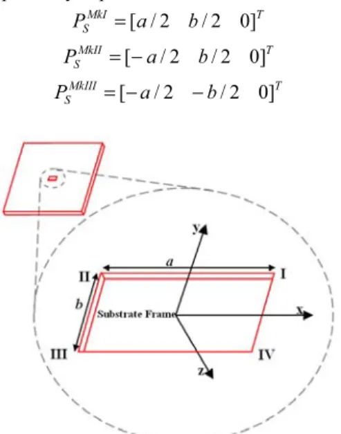
The substrate (Fig. 3) used in the calibration, is fabricated with four reference markers which are the corners of a square hole. So each marker on the substrate can be expressed as a vector in the substrate frame, for example, marker I, II and III can be respectively expressed as.

T MkI S a b P =[ /2 /2 0] T MkII S a b P =[− /2 /2 0] T MkIII S a b P =[− /2 − /2 0]

Fig. 3. The sketch of the substrate used in the calibration implementation of the micro force measurement system.

1) Estimation of R_RS

Three markers on the substrate will contact the AFM probe tip respectively, which is realized by AFM scanning the corresponding corner on the substrate. During this process, the parallel robot system should move linearly with fixed zero orientation. When the specific marker is detected by the AFM, the corresponding position vector of the parallel robot system

[

]

T

i i i

X Y Z should be recorded. Since robot system moves

with zero orientation, the transformation between robot frame and world frame can be expressed as below when marker i (i=I, II or III) is detected. 1 0 0 0 1 0 0 0 1 0 0 0 1 i i R Wi i X Y T Z ª º « » « » =_{« »} « » ¬ ¼

The process of contact between the markers and the AFM tip means that different points (reference markers) are sent to the same point (AFM tip) in the world frame, which can be formulated as below, where i=I, II or III.

AFM Mki R S Mki W W Wi R S

P =P =T ⋅T ⋅P

Here we reduce the dimension of vectors AFM

W

P and Mki

W

P to

three dimensions via eliminating the last perspective element. So for different three markers’ detection, the equation above can be rewritten as a three-dimensional equation,

[ ]3 1

0

Mki Mkj R S Mki R S Mkj W W Wi R S Wj R S

P −P =T ⋅T ⋅P −T ⋅T ⋅P = _× (1)

where i, j = I, II or III and i ำ j. So two independent

three-dimensional equations can be formulated, which can be

rewritten as six algebraic equations. As discussion above,

R Wi

T is a known matrix, so in the six algebraic equations there will be six unknown parameters which come from the

matrix S

R

T . However, when the equations (1) are expanded, it will be found the three parameters of the translation are eliminated and only three parameters of orientation are involved in equations. That means three unknown parameter should be solved from six independent equations, that is, a typical redundant calculation problem, which will be discussed in the following section. So, the rotation matrix

S R

R is solved via the method adopted. 2) Estimation of S

R

t and A W

t

Based on the solution of substrate orientation with respect to the robot system, the translation vector S

R

t also can be

solved via the similar operations. During this process, the three markers will be sent to the AFM probe tip again with a fixed orientation of the robot system. Just as mentioned above, the marker’s detection is also performed via AFM scanning. For the scanning, the parallel robot system also should move linearly, but the fixed orientation

[

θ_X θ_Y θ_Z

]

T should be recorded. When the marker is detected by AFM, the corresponding position of the robot system

[

Xi Yi Zi

]

Twill

also be recorded. So for the i th (i=I, II or III) detection, the transformation between robot frame and world frame, R

Wi

T can be expressed using

[

θ_Xi θ_Yi θ_Zi X_i Y_i Z_i

]

T.

The process of sending the same marker (for example marker I) to AFM tip means that the same point is sent for three times to the same point (AFM tip) in the world frame but the robot orientations are different, which can be formulated as below (i=1, 2 and 3).

AFM MkI R S MkI W Wi Wi R S

P =P =T ⋅T ⋅P

Here we also reduce the dimension of vectors AFM

W

P and

Mki W

P to three dimensions via eliminating the last perspective element. So for three markers detection, the equation above can be rewritten as a three-dimensional equation,

[ ]3 1

0

Mki Mkj R S Mki R S Mkj W W Wi R S Wj R S

P −P =T ⋅T ⋅P −T ⋅T ⋅P = _× (2)

where i, j = I, II or III and i ำ j. So two independent

three-dimensional equations can be formulated, which also can be rewritten as the form of six algebraic equations. R

Wi

T is a

known matrix for each time marker detection, so in the six algebraic equations there will be six unknown parameters

which come from the matrix S

R

T . In addition, the three orientation parameters have been solved above, so in the expanded equations (2), it will be found only three parameters about the translation involved in equations. The redundant equations can be solved via following the method, so the translation vector t is solved too. _RS

After the identification of matrix S R

T , we can utilize any marker detection data to calculate the translation vector A

W

which is the relative position of the AFM frame with respect to the world frame. It has been discussed above that any marker detection is performed based on the contact between the marker AFM tip point. So for example, we can use the data obtained during calibration of S

R

R to calculate the translation vector A

W

t , which can be formulated as below.

4 1 4 1 4 1 A AFM R S MkI W W WI R S t P T T P × × × ª º =ª º =ª ⋅ ⋅ º ¬ ¼ ¬ ¼ ¬ ¼ C. Algorithm

As mentioned above, during the first two steps of the calibration, the problem of redundant equations is encountered. In fact, it is the case that the number of the nonlinear equations is more than the number of the unknown parameters. So we have to find a set of solution to satisfy all the equations involved in the implementation, which is an optimization process. In addition, the equations generated during the orientation identification are nonlinear equations with cosine and sine operations. While a variety of methods are used in nonlinear equations solving or optimization implementation, in this research we employ a relatively straightforward and frequently used method, Gauss-Newton algorithm, to solve the nonlinear equations. The numerical solution based on Gauss-Newton method can be utilized directly in Matlab Optimization Toolbox.

III. EXPERIMENTALVALIDATION

A. Experiment setup

Fig. 4 shows the setup for the experiment of the kinematics parameter estimation. The robot integrated in the micro-force measurement system is a six degree-of-freedoms commercial parallel robot (product series: SpaceFab 3000 BS, MICOS, Germany), which can provide decades millimeters motion range (50mm×12mm×100mm) and sub-micrometers precision (0.2ȝm translation resolution and 0.0005o rotation resolution) [19]. The AFM (product model: SMENA, NT-MDT, Russia) employed in the micro-force measurement system, a compact and portable facility [20], will work as a force sensor in the future experiments, but during the period of kinematics parameters estimation it will work as a position sensor to detect the reference markers. In addition, a single degree-of-freedom piezoelectric actuated stage (P-611.ZS, PI, Germany) with nanometer level resolution [21] is fixed on the end-platform of the parallel robot system via a rigid holder, which provides high precision motion between the substrate and the AFM tip during the preload process. The parallel robot system and AFM system are fixed respectively on an anti-vibration table, which can effectively reduce the mechanical influence from the outside environment.

B. Standard substrate preparation

The substrate used in the experiment system is fabricated from silicon. The substrate is glued on the glass plate which is rigidly fixed on the end-platform of the piezoelectric stage. As the important parameters, the nominal dimension of the square hole is 3.6mm×0.8mm. The scanning electron microscope

picture of the substrate is shown in Fig. 5.

Fig. 4. The picture of experiment setup for the kinematics parameters estimation experiment.

Fig. 5. The SEM picture of the substrate used in the kinematics parameters estimation experiment.

C. Experiments

The detection of reference markers is a critical step for the system parameters estimation. In order to reduce the time measurement, we choose to minimize the number of scanning trajectories. In spite of scanning the corner using the AFM, only several points on each edges of the rectangle are scanned. So edges can be reconstructed and the identification of the corner can be calculated through the interaction of two adjacent edges. The edges of the square hole are relatively convenient to be identified, which can be realized by two curves scanning along the edge direction with a random spacing. Fig. 6 shows the camera view of the AFM cantilever and the edges to be scanned in the experiments.

0.8

3.6 mm

Parallel robot AFM head

Camera

Auxiliary light source PI stage & substrate holder AFM cantilever Substrate AFM cantilever Laser spot Edge to be scanned Cantilever holder

Fig. 6. The camera view of the substrate to be scanned and the AFM cantilever.

Before the curve scanning, an approaching motion will be implemented by a coarse motion and a fine motion, respectively. The parallel robot is utilized to make the substrate to approach the AFM tip in a relatively large motion range. After the substrate is very close to the AFM tip within micrometer level, the motion of the parallel robot is stopped and the piezoelectric stage is activated to continue to move the substrate towards the AFM tip until 50% of the AFM signal (about 2ȝm) is reached. After that, the scanning motion will be implemented in which the robot will move along X or Y axis respectively. The corresponding scanning curve is shown in Fig. 7. The blue curves are generated by the AFM scanning data, and red asterisk are the identified knee points which are determined based on the yellow lines. So the edge can be identified through the two knee points, which is shown in last sub-plot in Fig. 7. -3.48 -3.46 -3.44 -3.42 -15.973 -15.972 -15.971 X Axis Z A xi s -3.48 -3.46 -3.44 -3.42 -3.4 -15.966 -15.965 -15.964 X Axis Z Ax is -3.5 -3.45 -3.4 -3.35 -1 0 1 -15.98 -15.97 -15.96 X Axis Y Axis Z Ax is

Fig. 7. An example of the substrate edge identification through the scanning curves. (Blue lines: scanning data; red asterisks: identified knee points; pink line: identified edge)

The reference markers can be identified based on the results of the edges identification. Fig. 8 and 9 show the measurement curves, the identified edges and the identified corners. It is worthy to be mentioned that the four identified edges in the figures do not reflect the location of the physical square hole. In fact, the coordinate values of the points on the edges mean how the robot system needs to move when the corresponding points contact the AFM tip. Fig.8 shows the identification results when the orientation of the robot system is fixed to zero. According to the measurement data, if the markers I, II and III can contact the AFM tip respectively, the relative motion of the robot system are shown below

[

]

[

]

[

]

T MkIII S T MkII S T MkI S P P P 960 . 15 248 . 0 162 . 0 970 . 15 218 . 0 450 . 3 963 . 15 594 . 0 440 . 3 − − = − − − = − − =

Fig. 9 shows the measurement data and identification results, when the orientation of the robot system is set to 0.5o, -0.5o and 0.5o respectively. The motion of robot system is

listed below, when the markers I, II and III contact the AFM tip respectively.

[

]

[

]

[

]

T MkIII S T MkII S T MkI S P P P 219 . 16 293 . 0 407 . 0 260 . 16 282 . 0 203 . 3 249 . 16 531 . 0 200 . 3 − − = − − − = − − = -4 -3 -2 -1 0 1 -0.5 0 0.5 1 -15.98 -15.97 -15.96 -15.95 -15.94 X Axis Y Axis Z A xi s

Fig. 8. The measurement data and the edges identification result when the orientation of the robot system is fixed to zero. (Red lines: scanning data; blue lines: identified edges; black asterisks: identified corners)

-4 -3 -2 -1 0 1 -0.5 0 0.5 1 -16.28 -16.26 -16.24 -16.22 -16.2 X Axis Y Axis Z A xi s

Fig. 9. The measurement data and the edges identification result when the orientation of the robot system is fixed to 0.5o_{, -0.5}o _{and 0.5}o _{respectively.}

(Red lines: scanning data; blue lines: identified edges; black asterisks: identified corners)

According to the strategy mentioned in section II and the measurement data above, the kinematics parameters can be estimated as below. » » » » ¼ º « « « « ¬ ª − − − − = » ¼ º « ¬ ª = × 1 0 0 0 755 . 3 000 . 1 001 . 0 003 . 0 960 . 29 001 . 0 000 . 1 009 . 0 639 . 1 003 . 0 009 . 0 000 . 1 1 0₁₃ S R S R S R t R T

[

]

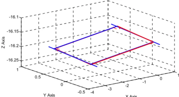
T A W t = 0.009 30.126 −19.714

In order to validate the estimation results, one more experiment is carried out, in which the orientation of the robot system is set to 0.4o -0.4o and 0.4o. The markers identification scanning experiment was repeated, whose results are shown in Fig. 10 (blue lines indicate the identified edges). On the other hand, based on the estimated parameters and the established model, the location of the marker points of the substrate also can be calculated, which is also shown in Fig.10 (red lines indicate the calculated edges). It can be seen the experiment

result and the calculation result match very well, in which the maximum error is maintained within the micrometer level.

-4 -3 -2 -1 0 1 -0.5 0 0.5 1 -16.25 -16.2 -16.15 -16.1 X Axis Y Axis Z A xi s

Fig. 10. The measurement data and the edges identification result when the orientation of the robot system is fixed to 0.4o_{, -0.4}o _{and 0.4}o _{respectively.}

(Blue lines: identified edges based on experiments; red lines: identified edges based on parameters estimation)

IV. CONCLUSION AND FUTURE WORKS

With the lack of effective experimental equipments, research on interaction and adhesion forces between planar micro-objects has been limited only to theoretical formulations or simulation. In this paper, an AFM/robot integrated system is introduced for micro-force measurement of plane/plane contact. As a necessary step, kinematics parameters estimation becomes a critical issue, which is focused and presented in this paper. A substrate with standard markers is employed as the pattern reference in the whole parameters estimation process, which utilizes the knowledge from the classical hand/eye calibration in robotics. Via a series of markers detection by AFM, the kinematics relationship involved in micro-force measurement system can be identified. Finally, the proposed parameters estimation method is validated through the experiments, which can be extended as a generic method to other AFM-based applications.

The proposed NANOROL system as an open research platform for the micro-force measurement is especially suitable for relatively complicated plane/plane contact study, which is the goal of the project. In the near future, a series of micro-force measurement of plane/plane contact, such as adhesion force, friction force and interaction force will be implemented on this system.

REFERENCES

[1] A. Mendez-Vilas, M. L. Gonzalez-Martin, L. Labajos-Broncano and M. J. Neuvo, “Experimental analysis of the influence of surface topography on the adhesion force as measured by an AFM,” Journal of Adhesion Science and technology, vol.16, no. 13, pp. 1737–1747, 2002.

[2] S. C. Chen and J. F. Lin, “Detailed modeling of the adhesion force between an AFM tip and a smooth flat surface under different humidity levels,” Journal of Micromechanics and Microengineering, vol. 18, 115006 (2008)

[3] K. Rabenorosoa, C. Clévy, P. Lutz, M. Gauthier and P. Rougeot, “Measurement of pull-off force for planar contact at the microscale,” Micro & Nano Letters, vol. 4, no. 3, pp. 148–154, 2009

[4] K. L. Johnson, K. Kendall, and A. D. Roberts, “Surface energy and the contract of elastic solids,” Proceedings of Royal Society A., vol.324, pp. 301–313, 1971.

[5] B. V. Derjaguin, V. M. Muller and YU. P. Toporov, “Effect of contact deformations on the adhesion of particles,” Journal of Colloid and

Interface Science, vol. 53, no. 2, pp. 314–326, November 1975.

[6] V. M. Muller, V. S. Yushchenko, and B. V. Derjaguin, “On the influence of molecular forces on the deformation of an elastic sphere and its sticking to a rigid plane,” Journal of Colloid and Interface

Science, vol. 77, no. 1, pp. 91–101, September 1980.

[7] R. Y. Tsai and R. K. Lenz, “Real time versatile robotics hand/eye calibration using 3D machine vision,” IEEE Transaction on Robotics

and Automation, vol. 1, pp. 554–561, June 1988.

[8] Y. C. Shiu and S. Ahmad, “Calibration of wrist-mounted robotic sensors by solving homogeneous transform equations of the form AX=XB,” IEEE Transaction on Robotics and Automation, vol. 5, no. 1, pp. 16–29, February 1989.

[9] J. Chou and M. Kamel, “Finding the position and orientation of a sensor on a robot manipulator using quaternions,” International

Journal of Robotics Research, vol. 10, no. 3, pp. 240–254, June 1991.

[10] H. Zhuang and Z. S. Roth, “Comments on ‘Calibration of wrist-mounted robotic sensors by solving homogeneous transform equations of the form AX=XB’,” IEEE Transaction on Robotics and

Automation, vol. 7, no. 6, pp. 877–878, December 1991.

[11] C. -C. Wang, “Extrinsic calibration of a vision sensor mounted on a robot,” IEEE Transaction on Robotics and Automation, vol. 8, no. 2, pp. 161–175, April 1992.

[12] L. -H. Robert, N. -D. Guilherme and C. -K. Avinash, “An iterative approach to the hand-eye and base-world calibration problem,” in

IEEE International Conference on Robotics and Automation (ICRA2001), Seoul, Korea, May 2001, pp. 2171–2176.

[13] H. Malm and A. Heyden, “Simplified intrinsic camera calibration and hand-eye calibration for robot vision,” in IEEE/RSJ International

Conference on Intelligent Robots and systems (IROS 2003), Las Vegas,

USA, October 2003, pp. 1037–1043.

[14] K. H. Strobl and G. Hirzinger, “Optimal hand-eye calibration,” in

IEEE/RSJ International Conference on Intelligent Robots and systems (IROS 2006), Beijing, China, October 2006, pp. 4647–4653.

[15] R. -R Jorge, H. -G. Silena and B. -C. Eduardo, “Geometric hand/eye calibration for an endoscopic neurosurgery system,” in IEEE

International Conference on Robotics and Automation (ICRA2008),

Pasadena, USA, May 2008, pp. 1418–1423.

[16] A. Jordt, N. T. Siebel and G. Sommer, “Automatic high-precision self-calibration of camera-robot systems,” in IEEE International

Conference on Robotics and Automation (ICRA2009), Kobe, Japan,

May 2009, pp. 1244–1249.

[17] W. Yashiro, I. Shiraki and K. Miki, “A probe-positioning method with two-dimensional calibration pattern for micro-multi-point probes,” Review of Scientific Instruments, vol. 74, no. 5, pp. 345–358, May 2003.

[18] H. Bilen, M. A. Hocaoglu, E. A. Baran, M. Unel and D. Gozuacik, “Novel parameter estimation schemes in microsystems,” in IEEE International Conference on Robotics and Automation (ICRA2009), Kobe, Japan, May 2009, pp. 2394–2399.

[19] http://www.micos-online.com/web2/en/1,3,010,sf3000bs.html [20] http://www.ntmdt.com/device/smena

[21] http://www.physikinstrumente.com/en/products/prspecs.php?sortnr=2 01730