CNS: a GPU-based framework for simulating cortically-organized networks

Computer Science and Artificial Intelligence Laboratory

Technical Report

MIT-CSAIL-TR-2010-013

CBCL-286

February 26, 2010

CNS: a GPU-based framework for

simulating cortically-organized networks

Jim Mutch, Ulf Knoblich, and Tomaso Poggio

CNS: a GPU-based framework for simulating cortically-organized networks

Jim Mutch

_{, Ulf Knoblich, and Tomaso Poggio}

Center for Biological and Computational Learning

McGovern Institute for Brain Research

Massachusetts Institute of Technology

Cambridge, MA

[email protected], [email protected], [email protected]

Abstract

Computational models whose organization is inspired by the cortex are increasing in both number and popularity. Current instances of such models include convolutional net-works, HMAX, Hierarchical Temporal Memory, and deep belief networks. These models present two practical chal-lenges. First, they are computationally intensive. Second, while the operations performed by individual cells, or units, are typically simple, the code needed to keep track of net-work connectivity can quickly become complicated, leading to programs that are difficult to write and to modify. Mas-sively parallel commodity computing hardware has recently become available in the form of general-purpose GPUs. This helps address the first problem but exacerbates the sec-ond. GPU programming adds an extra layer of difficulty, further discouraging exploration.

To address these concerns, we have created a program-ming framework called CNS (’Cortical Network Simula-tor’). CNS models are automatically compiled and run on a GPU, typically 80-100x faster than on a single CPU, with-out the user having to learn any GPU programming. A novel scheme for the parametric specification of network connectivity allows the user to focus on writing just the code executed by a single cell. We hope that the ability to rapidly define and run cortically-inspired models will facilitate re-search in the cortical modeling community. CNS is avail-able1under the GNU General Public License.

1. Introduction

1.1. Definitions

For the purpose of this paper, we define a ’cortical’ model to be a network model which consists of some number of

∗_{Author to whom correspondence should be addressed.}

1_{Software and a full programming manual are available at}

http://cbcl.mit.edu/jmutch/cns.

N-dimensional ’layers’ of cells, where each layer encodes some N-D feature space. It is common for at least some of the dimensions to be topographically mapped, meaning that physical proximity in the layer corresponds to proxim-ity in the feature space. N, and the feature space, can be the same or different from layer to layer. All the cells in a layer must be of the same type, i.e., each maintains its own val-ues of the same set of variables, using the same algorithm. Connectivity between cells may be completely arbitrary, but often consists of a repeating pattern.

This class of models includes, but is by no means limited to:

• Convolutional networks [5,4]. • HMAX [9,8].

• Hierarchical Temporal Memory [1]. • Deep belief networks [2].

• Detailed spiking models of cortex.

Some of these are ’static’ models, requiring only a single pass through the network for a given input. Others have dynamics that require iteration over many time steps.

1.2. Motivation

Cortical models commonly contain a large number of units

and are therefore computationally expensive. However,

they are highly amenable to parallelization. The layered structure of cortical models maps very well to the architec-ture of modern GPUs, which are optimized to perform the same operation at every point in an array of data. GPUs have evolved from graphics accelerator cards, where the ar-ray elements are pixels. Over the last few years the APIs for these cards have opened up to encourage the accelera-tion of non-graphical algorithms that can benefit from the same architecture. Current GPUs have hundreds of paral-lel processors and can typically run suitable algorithms 80-100x faster than a single CPU. However, these performance

gains are not free. A GPU’s processors all still share a com-mon memory, which becomes the bottleneck of the system. To achieve optimal performance, GPU programmers must code their algorithms so that the processors access memory in coordinated patterns. This adds another layer of diffi-culty to models that can already be somewhat challenging to program.

Individual cells in cortical models typically perform fairly simple functions. Difficulties in programming these models usually arise in keeping track of the connectivity between cells. There are two common approaches:

• Enumerate every synapse. With this approach, one can represent any network architecture, but for net-works having regular patterns of connectivity, it is ex-tremely wasteful. Memory usage increases drastically, and because memory access is the bottleneck in multi-processing systems, so does multi-processing time.

• Matrix operations. This is a common abstraction that works for some simple hierarchical models. Layer n is

generated from layer n− 1 via some matrix operation

such as N-D convolution. This is very space-efficient and easy to implement in a language such as MAT-LAB. It is also fairly straightforward to implement on a GPU, and to program arbitrary response functions in place of the dot product implied by convolution. However, in more complex situations this abstraction becomes limiting. Actual cortical areas typically re-ceive convergent input from multiple pathways that have been processed differently. Operations may have been carried out at different resolutions, or the number of processing steps may have been different. Thus, the indices of cells in two different input layers no longer have the same meaning, and it is difficult to define a matrix operation that combines them. Most work in cortical modeling has simply focused on the subset of models for which these difficulties do not arise. Of the two barriers to exploration of the cortical model space – programming time and run time – GPU program-ming alone can only address the latter, and at the expense of the former. A framework is needed that can address both issues.

1.3. Overview of CNS

CNS is a rapid development environment for cortical mod-els. Models are compiled and run automatically on NVIDIA GPUs, often running 80-100x faster than on a single CPU, without the user having to learn any GPU programming.

Most aspects of a model are defined via MATLAB scripts, including:

• The number of layers.

• The dimension, size, and cell type of each layer. • The variables associated with each cell type, and their

initial values.

• The connectivity between cells.

The process of running models, loading input data, and pulling back results is also controlled via MATLAB. Vari-ables are referred to by name – the user does not need to be concerned with where they are stored in GPU memory.

There are two options for specifying connectivity. As in many other simulators, synapses may be explicitly enumer-ated: a given cell can list any number of presynaptic cells, which can be in any layer. For models having regular pat-terns of connectivity, CNS uses a scheme in which each cell explicitly retains its grid position (the center of its recep-tive field) in a real-valued feature space which is meaningful across layers. For example, in a vision model, the dimen-sions of this common feature space would probably include retinal position, and even cells several steps removed from the input would still know their center coordinates in reti-nal space. Under this scheme, cells can infer their inputs based on proximity in the common feature space. By appro-priate relative arrangement of the coordinate grids for each layer, any of the standard connectivity patterns (e.g., valid and full convolution, sub- and super-sampling, etc.) can be achieved, as well as many others. Once defined in this way, connectivity is handled by the framework. An individual cell can make requests of the framework, for example, it can request the indices of its n nearest neighbors in layer z. This division of labor allows programmers to focus mainly on the code being executed by a single cell.

A ’kernel’ is the code each cell executes during an itera-tion of the network. Cells of the same type share the same kernel. Kernels run on the GPU and are the only parts of a CNS model that must be written in C/C++. Even when writing a kernel, however, the programmer remains isolated from the complexities of the GPU. A kernel is written from the point of view of a single cell, so the programmer is not responsible for any thread scheduling. Nor is the program-mer required to know where variables are stored in GPU memory. CNS provides named macros that the kernel can call to, among other things:

• Read and write the current cell’s variables.

• Find input cells via proximity in the feature space, as described above.

• Read the values of other cells’ variables.

During model development, CNS can be thought of as a compiler, in that programmers do not need to read or mod-ify any of CNS’s code. By way of comparison, the 3-D convolutional network package with backpropagation

300 lines, while CNS itself is about 10,000 lines as of this writing.

CNS is licensed under the GNU General Public License. The software and programmer’s manual are available at http://cbcl.mit.edu/jmutch/cns.

1.4. Structure of this paper

The remaining sections of this paper are as follows: • Section2introduces three example packages written

in CNS.

• Section3discusses some CNS concepts in more detail, using the example packages for illustration.

• Section4describes the process of developing and run-ning a CNS model.

• Section5provides some internal details on how CNS maps models to the GPU architecture.

• Section6lists some limitations of CNS. • Section7outlines future work on CNS.

This paper is intended as a high-level introduction to CNS. Exact syntax is not covered beyond a few examples. For a complete description of all CNS syntax and options, see the

programmer’s manual [6].

2. Example packages

In CNS, a ’package’ is a collection of cell types that is used to construct models. For example, the ’HH’ package de-scribed below implements several types of Hodgkin-Huxley cells. Once you have a package, you can then build net-works consisting of those types of cells. The same package can be used to define many specific models, having different numbers of layers, of different sizes, with different connec-tivity, etc.

In this section we briefly describe three packages that we have developed with CNS. Subsequent sections will refer back to these examples to illustrate various CNS concepts.

2.1. ’HH’ package: Hodgkin-Huxley spiking

mod-els

The Hodgkin-Huxley (HH) package is used to build models made up of 2-D layers of spiking neurons, similar to the

cortical laminae. Figure1shows part of three layers of such

a model:

• IN: the input layer. Each cell has its own list of prepro-grammed spike times.

• F1: a layer of fast-spiking inhibitory cells, each receiv-ing input from a local region of IN.

• P1: a layer of pyramidal cells, each receiving input from a local region of IN and F1 (latter connections not shown).

IN

(input)

F1

(wb)

P1

(ga)

Y x X

Y x X

Y x X

Dimension

Names:

Layer Name:

(type)

Figure 1. Schematic of part of a model made up of Hodgkin-Huxley spiking neurons (see section2.1), implementing monosy-naptic excitation with disymonosy-naptic inhibition. IN: input layer. F1: fast-spiking inhibitory cells (Wang-Buzsaki model). P1: pyrami-dal cells (Golomb-Amitai model). IN-P1 connections, and other layers, are not shown. The full model contained 10,000 cells.

0 0.2 0.4 0.6 −60 −40 −20 0 Time (s) Membrane Potential (mV)

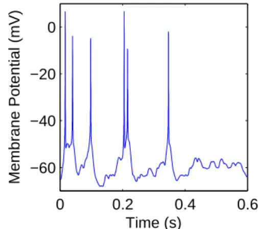
Figure 2. Voltage trace output for one cell in a Hodgkin-Huxley model (see section2.1).

In these models, cells in a layer are assigned to grid posi-tions in a 2-D feature space, but with some gaussian noise added. Connectivity is also noisy; for example, each F1 cell receives input from a local region of IN cells, but with the probability of a connection decreasing with distance from the center of the region. Thus, connectivity in these models is defined using the explicit synapses method: each cell in a model lists its presynaptic cells.

Models built with this package are dynamic. Each cell maintains its own set of Hodgkin-Huxley state variables. Each iteration of the network represents a small time step, during which each cell polls its presynaptic cells to see which ones are spiking and updates its state variables ac-cording to a set of differential equations. CNS can track the

values of selected state variables as they change; figure2

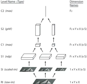
1 x Y x X (x S) 1 x Y x X F1 x Y x X (x S) F1 x Y x X (x S) F2 x Y x X (x S) F2 S1 (ndp) C1 (max) S2 (grbf) C2 (max)

Level Name (Type) Dimension

Names

SI (scaled-im)

RI (raw-im)

Figure 3. An example of an HMAX model (see section2.2). Each step is performed at multiple scales, only three of which are shown here.

For a model with 10,000 neurons and 330,000 synapses, CNS was able to process 5,000 time steps per second on a GTX 285 GPU.

2.2. ’FH’ package: HMAX-like feature hierarchies

[9,8] class. HMAX models the initial feedforward stage of

object recognition in the ventral visual pathway. It extend

the idea of simple and complex cells [3] to form a

hierar-chy in which alternating template matching and max pool-ing operations progressively build up both feature

selectiv-ity and invariance to position and scale. Figure3illustrates

one such model [8] as it is expressed in CNS.

HMAX is scale invariant: each stage of processing is carried out at multiple scales. Thus, each stage of the model is actually represented by many CNS layers, one for each

scale. For the model in figure3, the stages are:

• SI: Many different resolutions of the original image, produced by bicubic interpolation.

• S1: Applies gabor filters of several orientations at

ev-ery position and scale. Each scale is now of size

F1× Y × X, where F1is the number of orientations. • C1: Independently for each orientation, computes the

maximum response over a local area of position and scale. Also subsamples by a factor of 5. Note that the operation of pooling over multiple scales would be difficult to define as a matrix operation. Here it is done using CNS’s common coordinate scheme (see section3.6).

• S2: Computes the response to many stored templates at every position and scale. Now in each scale we have F2×Y ×X units, where F2is the number of templates. • C2: For each template, finds the maximum response over all positions and scales. This results in a feature vector which can be fed into a classifier.

These models are computed in a single bottom-up pass for a given input image. The gabor filters in S1 and the stored templates in S2 are shared by all the cells in those layers

(and are not shown in figure3).

The FH package replaces an older CPU-based library

called FHLib [7] which was used for the experiments in [8].

For one large model, CNS outperformed FHLib by a factor of 97x on a GTX 285 GPU.

2.3. ’CN’ package: convolutional networks for 3-D

image segmentation

The ’CN’ package is a CNS reimplementation of the code

used in [4]. It is used to train and run convolutional

net-works that perform segmentation in 3-D electron micro-scope images of brain tissue. These networks are similar

to those of Lecun [5] except that the filters have three

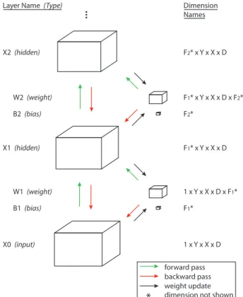
spa-tial dimensions and there is no subsampling. The model architecture is illustrated in figure4.

Each Xilayer is four-dimensional, containing the value

of Fidifferent features at each position in a 3-D cube. (For

the input image X0 there is only one feature: the pixel

value.) The features are different in each stage. Each Wi

can be viewed as Fifour-dimensional filters which, via

con-volution over Xi

−1 (and then adding the appropriate bias

from Bi), produce layer Xi. Note that convolution only

occurs over the three spatial dimensions; for the feature

di-mension, Xi₋1and the filter are the same size.

The goal of the training phase is to learn all the Wi and

Bi layers. This is done via the backpropagation algorithm

in three passes (mathematics in [4]):

• Forward pass: starting with the input in X0, compute

the outputs of each Xilayer from bottom to top.

• Backward pass: starting with the desired output in Xn,

compute the error term (’sensitivity’) for each Xifrom

top to bottom.

• Weight update: update each Wiand Bilayer.

Note that unlike the filters and features in FH models (sec-tion2.2), here the weights and biases need to change during a network iteration. Thus, we treat them as layers, and they have their own kernels which perform the update at the ap-propriate time.

Once the network has been trained, only the forward pass is needed to perform segmentation.

X2 (hidden) X1 (hidden) X0 (input) W2 (weight) B2 (bias) W1 (weight) B1 (bias) F2* x Y x X x D F1* x Y x X x D 1 x Y x X x D F1* x Y x X x D x F2* 1 x Y x X x D x F1* F2* F1*

Layer Name (Type) Dimension

Names

*

forward pass backward pass weight update dimension not shown

...

Figure 4. The first three stages of a convolutional network for seg-menting 3-D images (see section2.3).

The CNS implementation of this class of models ran about 100x faster than the previous code, based on timing using a single CPU. Ongoing development of these models continues under CNS.

3. CNS concepts

In this section we run through the key concepts of CNS,

using the packages in section2as examples.

3.1. Layers and groups of layers

The basic architectural unit of a CNS model is the layer, which is an N-dimensional array of cells that are all of the

same type (see section3.3). Practically speaking, a model

can have up to several hundred layers. Note that layers do not have to be arranged in any kind of hierarchy or directed acyclic graph (DAG).

Multiple layers of the same type can be designated as a group. The main purpose of this is to allow them to share some common data. For example, in the FH package, all the S1 layers (of different scales) are designated as a group so they can share the same set of precomputed gabor filters.

3.2. Execution order

By default, a single network iteration consists of computing all cells in all layers exactly once, in parallel. HH models work like this. Internally, of course, everything isn’t com-puted exactly at once. A double-buffering system is em-ployed to guarantee that during iteration t, all the values a

kernel reads from other cells come from iteration t− 1.

For some models, it wouldn’t make sense to compute all the layers at the same time. For example, cells in FH mod-els do not have states that evolve over time. There is no

point in computing layer n until layer n− 1 has been

com-puted. In this case, a network iteration is broken into steps,

with layers assigned different step numbers. In figure3, for

example, all the SI layers are assigned step 1, the S1 layers step 2, the C1 layers step 3, etc.

CN models are similar to FH, except that a single iter-ation consists of a forward pass, a backward pass, and a

weight update. The Xilayers get computed at two different

points in one iteration, i.e., they each have two different step numbers, and perform a different computation in each.

Note that there is no unit of execution smaller than a sin-gle layer.

3.3. Cell types

• The dimensionality (N) a layer of cells of that type must have. For example, all the layers in HH

mod-els are 2-D, but in CN modmod-els the Xi layers are 4-D,

the Wilayers are 5-D, and the Bilayers are 1-D.

• The constants and variables (fields) associated with each cell. (Fields can also have layer scope, synapse

scope, etc.; see section3.4.)

• The kernel used to update a cell during a network

iter-ation (see section3.5).

Just like a class in object-oriented programming, a cell type can be a subtype of a parent type. All the cell types in a package form a type hierarchy (not to be confused with a model having hierarchical structure). Every package must have a ’base’ type which is the root of the type hierarchy. A cell type inherits the following properties from its parent type:

• The dimensionality of a layer. Note that this cannot be overridden.

• All fields.

• The kernel. This can be overridden.

Cell types can be abstract, which means they exist only to declare a common set of properties that are then inherited

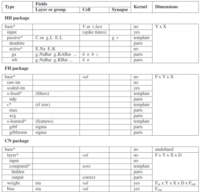
Type Fields Kernel Dimensions Layer or group Cell Synapse

HH package

base* V m t last no Y x X

input (spike times) yes

passive* C m g L E L g r template

dendrite parts

active* E Na E K no

ga g NaBar g KABar ... h n b z parts

wb g NaBar g KBar ... h n parts

FH package

base* val no F x Y x X

raw-im no

scaled-im yes

s-fixed* (filters) template

ndp parts

c* (rf size) template

max parts

avg parts

s-learned* (features) template

grbf sigma parts

grbfnorm sigma parts

CN package

base* no undefined

layer* val no F x Y x X x D

input no

computed* sens template

hidden parts

output correct parts

weight eta val yes Finx Y x X x D x Fout

bias eta val yes Fout

Table 1. Cell types for the example packages. Indentation in the ’type’ column denotes inheritance, and * denotes an abstract type. Italicized fields are read-write, i.e., variable. Note that a cell type inherits all its parent type’s fields.

by subtypes. In many packages, the ’base’ type will be ab-stract. You cannot create layers of cells of an abstract type; you must use a non-abstract subtype.

Table1 shows the type hierarchy for all three example

packages.

3.4. Fields and scope

In CNS, a named numeric quantity associated with a cell is called a field. For example, in HH models, membrane volt-age (V m) is a field, and each cell maintains its own value of the membrane voltage. For cells, fields are analogous to the data members of a class or structure in object-oriented programming. Each cell type inherits its parent type’s fields and may also define its own fields. The definition of a field includes:

• Field name. Used to identify the field, both in the MATLAB interface and inside kernels.

• Data type: either single-precision floating point or 32-bit signed integer.

• Scalar or vector.

• Read-only or read-write. Read-only fields (constants) cannot change their values during a model iteration on the GPU, but they can be changed between iterations from within MATLAB. Read-write fields (variables) may be changed during a model iteration, but only for the current cell, i.e., each cell is responsible for updat-ing its own variables.

is initialized. May be overridden at model initialization time. If no default value is defined, then one must be given at model initialization time.

• Scope: see below.

One key way in which CNS fields are not like data members in object-oriented programming is that you can also define their scope. A field can have:

• Cell scope. Each cell maintains its own value of the field. (If the field is a vector, each cell maintains its own vector value. This applies to all the scopes listed here.)

• Synapse scope. Available when using

explicit-synapses connectivity (section3.6). A separate value

of the field is maintained for each synapse. This can obviously take a lot of memory.

• Layer scope. Each layer will have one value of the field that applies to the whole layer. Such fields are always read-only.

• Group scope. One (read-only) value of the field is maintained for an entire group of layers (see sec-tion3.1).

• Model scope. One (read-only) value of the field is maintained for an entire network model.

Table1 shows many of the fields defined by the example

packages.

One more kind of field is also available. In some models it is desirable for many cells to have access to the same large multidimensional array of static data. One way of doing this would be to use the same approach the CN package uses

to share Wi and Bi values, which is to make such arrays

into layers of their own. In CN models, Wiand Bi are not

static, so this is the only option. In the FH model shown

in figure3, however, the S1 stage’s gabor filters and the S2

stage’s stored features are static during a network iteration, so it would be nice to not have to complicate the network structure by making them separate layers. CNS allows static arrays like this to be defined as fields having layer, group, or model scope.

3.5. Kernels

A kernel is a function that updates a cell’s variables during a network iteration. As with methods in object-oriented pro-gramming, a kernel is written from the point of view of a single cell. Unlike object-oriented programming, however, each cell type has exactly one kernel.

Kernels are written using a limited subset of C++ (mostly just C), supplemented by macros generated by CNS. You may provide an arbitrary block of C/C++ code, subject to these conditions:

• Only statements that are permissible in function scope (inside a function body) are allowed.

• The only standard library functions available are those in the ’math’ library.

• No dynamic memory allocation is permitted.

Access to fields and other properties you have defined for the various cell types is done via macros that CNS provides. This spares you from having to worry about how data is laid

out in GPU memory, etc. Figure5shows part of a kernel

from the CN package; all the red symbols are macros gen-erated by CNS, based on the definitions for cell types in that package.

When you are writing a kernel, you can ask CNS to list all the macros available to you. CNS provides macros to:

• Read and write fields. (For example, the READ *

macros,WRITE VAL,ZP,ZW, andZBin figure5.)

• Retrieve current cell coordinates. (For example,

THIS Fin figure5.)

• Find receptive fields. (For example, the* RF NEAR

macros in figure5.)

• Retrieve layer dimension sizes. (For example, the

* SIZEmacros in figure5.)

• Loop through explicit synapses, if any.

• Retrieve the current iteration number and other miscel-lanea.

Closely related kernels are often very similar. For example, one might want to define a cell type having a kernel like the

one in figure5, but with the dot product operation, or

per-haps the sigmoid nonlinearity, replaced by something else. To avoid having many kernels that are slightly-modified copies of one another, CNS allows you to write a template kernel for an abstract parent type. The template kernel will contain most of the logic, leaving ’blanks’ for the specific operations. Then the various subtype kernels provide differ-ent code snippets (parts) that ’fill in’ those blanks for each subtype. This feature is used in all three example packages;

see the ’kernel’ column in table1.

3.6. Connectivity

As discussed in sections1.2and1.3, CNS has two ways to

specify cell-to-cell connectivity:

• HH models use the explicit synapses method: each cell lists each of its presynaptic cells. This is necessary because cells in HH models do not occupy regular grid positions in a common feature space.

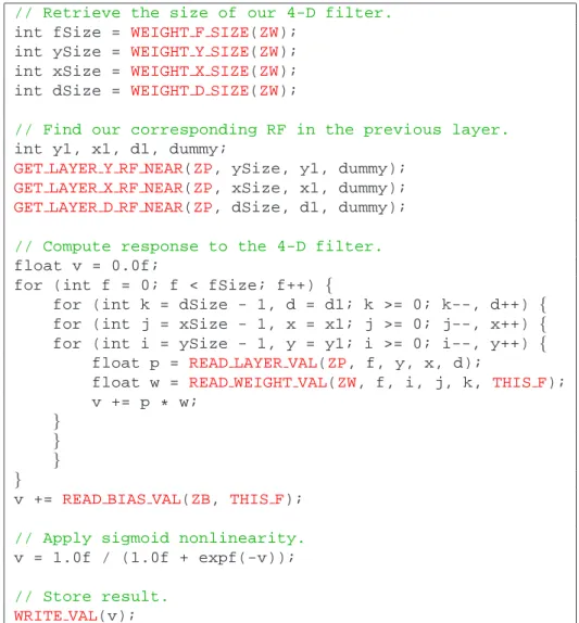
// Retrieve the size of our 4-D filter.

int fSize = WEIGHT F SIZE(ZW);

int ySize = WEIGHT Y SIZE(ZW);

int xSize = WEIGHT X SIZE(ZW);

int dSize = WEIGHT D SIZE(ZW);

// Find our corresponding RF in the previous layer.

int y1, x1, d1, dummy;

GET LAYER Y RF NEAR(ZP, ySize, y1, dummy);

GET LAYER X RF NEAR(ZP, xSize, x1, dummy);

GET LAYER D RF NEAR(ZP, dSize, d1, dummy);

// Compute response to the 4-D filter.

float v = 0.0f;

for (int f = 0; f < fSize; f++) {

for (int k = dSize - 1, d = d1; k >= 0; k--, d++) {

for (int j = xSize - 1, x = x1; j >= 0; j--, x++) {

for (int i = ySize - 1, y = y1; i >= 0; i--, y++) {

float p = READ LAYER VAL(ZP, f, y, x, d);

float w = READ WEIGHT VAL(ZW, f, i, j, k, THIS F);

v += p * w;

} } } }

v += READ BIAS VAL(ZB, THIS F);

// Apply sigmoid nonlinearity.

v = 1.0f / (1.0f + expf(-v));

// Store result.

WRITE VAL(v);

Figure 5. Part of a kernel from the CN package. This code performs the forward pass. It computes the value of a single cell in an Xilayer

by overlaying the appropriate 4-D weight array from Wionto the cell’s 4-D receptive field in X_i−1, computing the dot product, adding the

appropriate bias from Bi, and applying a sigmoid nonlinearity. Symbols inREDare macros generated by CNS; everything else is standard

C/C++. See section3.5for details.

• FH and CN models use the common coordinates method. Here we expand a bit on that topic.

In FH models, the dimensions Y and X correspond to reti-nal position and are meaningful across all layers. In CN,

the same holds in the Xilayers for spatial dimensions Y, X,

and D (depth). Thus, cells in both packages are assigned to real-valued grid positions in these common dimensions.

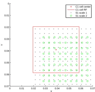
Figure6 illustrates how these coordinates are used to

per-form an operation (pooling over scales that are not an inte-ger multiple of one another in an FH model) that is difficult to define without them.

Note that this is just one instance of a general problem which can arise in several ways, and which CNS’s common coordinate system was designed to solve: how does one de-fine ’local’ operations like convolution over multiple layers

having different sizes, resolutions, etc.? Networks having multiple pathways that converge will almost always have this issue, since the different pathways probably involve dif-ferent amounts of convolution (with edge loss) and/or sub-sampling. And of course, convergence occurs throughout cortex.

Part of defining a network model in CNS is setting up

these grid positions for the different layers. There is a

function (cns mapdim) that handles all the standard cases:

valid, same, and invalid convolutions, subsampling, super-sampling, etc. Once grid positions have been assigned, con-nectivity is handled by CNS - in kernel code, you simply call a macro requesting, for example, the nearest n neigh-bors in some layer z, or every cell within radius r.

Not all dimensions in a model need to have a common coordinate system. For example, the non-spatial

dimen-0 0.01 0.02 0.03 0.04 0.05 0.06 0.07 0 0.01 0.02 0.03 0.04 0.05 0.06 0.07 X Y C1 cell center C1 cell RF S1 scale 1 S1 scale 2

Figure 6. Common coordinate positions for several layers of an FH model. The C1 cell shown is a corner cell of a layer that has been arranged to perform a 10x10 valid convolution over the layer representing the first S1 scale. The second S1 scale’s cells do not line up with either of the other two layers shown; however, it is still possible to define a pooling operation over both S1 layers – the C1 cell just takes a max over any cell in its receptive field.

sions in FH and CN models do not have the notion of lo-cality, so for them this scheme is not used.

4. Working with CNS

In this section we provide a quick overview of the process of developing and running CNS models.

Before you can build a network model, you must define your cell types. This is done by creating a package, which is a collection of related cell types, or by acquiring and pos-sibly modifying an existing package. For example, if you wanted to build a network of Hodgkin-Huxley spiking cells, you would probably want to start with the existing HH pack-age. The properties of cell types and their associated fields

and kernels are described in sections3.3,3.4, and3.5. Most

of these definitions are made in MATLAB ’.m’ files, with kernels in C/C++ ’.h’ files. All such files for a single pack-age are stored together in a packpack-age directory. Before you can use a package, it must be compiled into an executable

using thecns buildcommand. This actually produces

two executables, one that runs models on a GPU and an-other that runs models on a CPU. The latter option can be useful for development and debugging.

Once you have a compiled package, you can use it to build and run any number of different network models,

hav-ing different numbers and sizes of layers, with different con-nectivity, etc. The process of building and running a net-work model is as follows. All steps are carried out from within MATLAB using a few CNS commands.

1. Define the structure of your network: the number of layers, their sizes and types, cell-to-cell connectivity, and the initial values of fields. This is all defined in a MATLAB struct which you create. The helper func-tioncns mapdimcan assist you in setting up a

com-mon coordinate system (section3.6).

2. Initialize the model on the GPU (or CPU). This can take a few seconds.

3. Run the model for any number of iterations.

• For dynamic models (e.g. HH models) this may involve loading some input data and then letting the model iterate for awhile. Variables can be tracked as they change, or if you just want their final values, you can pull them out when all iter-ations are complete.

• Other models (e.g. FH models) process their in-put in a single iteration. For these models you simply load your input data, perform a single it-eration, and pull out any output data. For batch operations (e.g., processing many images with an FH model) you would perform those three oper-ations inside a loop.

4. Deallocate the model, freeing resources.

5. GPU details

While there are some circumstances in which model choices have performance consequences – these are documented in

the programmer’s manual [6] – users in general do not need

to understand GPU programming in order to use CNS. Here we provide a few details on how CNS works

behind the scenes. This section is intended for those

familiar with GPU programming concepts; an exposition of GPU programming and architecture is beyond the scope of this paper.

Dimension mapping. The user sees layers as N-dimensional arrays, and this abstraction is consistent throughout CNS: both MATLAB functions and kernel macros view layers as N-D. However, internally layers are stored as 2-D. This is done because some fields need to be stored in GPU textures (see below). Textures can be 2-D or 3-D, but for 3-D textures the size limits are prohibitively small as of this writing. It is also more difficult to do texture packing in 3-D. Thus, CNS uses only 2-D textures.

All translation between N-D and 2-D is handled by CNS. The user’s only involvement in this process occurs when defining a cell type. The user must choose the internal dimension (Y or X) to which each external dimension is mapped. Current GPU limits on texture size will influence these decisions. When two or more external dimensions are mapped to the same internal dimension, the user must

also specify the nesting order. This choice has

perfor-mance consequences. Storage will only be contiguous

for the innermost dimension, so kernels involving nested loops should iterate over the innermost dimension in the

innermost loop. (This is done in figure5.) CNS

automati-cally pads the innermost Y dimension to the warp size so that warps will perform coalesced reads as often as possible.

Types of GPU memory. CNS automatically maps each

field to the appropriate kind of GPU memory based on the field’s definition:

• Small, shared constants having layer, group, or model scope are stored in the constant cache. The constant cache is also used to store internal metadata such as layer sizes.

• Fields that have cell scope and that will be read by other cells are stored in textures. One texture is used for all the layers having that field; texture packing is done automatically.

• Everything else goes into global memory. • Shared memory is not used.

Blocks and threads. All layers having the same cell type

are evaluated in a single kernel call (unless the user has

as-signed them to different step numbers; see section3.2). The

decomposition into blocks and threads is done automati-cally. Each cell gets its own thread. Each layer becomes one or more thread blocks; an individual thread block will contain threads from a single layer only. Blocks are 2-D and aligned in the same way as memory (see above) to maxi-mize the number of coalesced reads and the benefits of tex-ture caching.

6. Limitations

6.1. Inherent Limitations

The following limitations are inherent in CNS’s role as a rapid development framework for expressing arbitrary mod-els having a cortical organization:

• CNS implements a generic, automatic process for mapping cortical models to the GPU architecture. For any given specific model, it will always be possible for a sufficiently skilled programmer to write custom

GPU code that runs faster by taking advantage of opti-mization techniques peculiar to that model. However, custom GPU code is much harder to write and mod-ify. The speedups we are seeing under CNS relative to a single CPU (80-100x) are on the order of what is typically reported in the literature for direct GPU im-plementations of various algorithms. Our testing so far suggests that, at worst, a CNS model will be no more than 2x slower than a carefully-written custom GPU implementation of that specific model.

• Models must run inside a single GPU. Host-GPU com-munication is relatively slow, and CNS makes no as-sumptions about the sparsity of long-range vs. local connectivity, nor about the frequency of cell-to-cell communication. A less general framework in which such assumptions could be made might be able to au-tomatically decompose models into pieces that could run on separate GPUs without incurring prohibitive

data transfer delays. CNS cannot do this, so any

such decomposition must be done by the user, outside CNS. Barring a dramatic improvement in the speed of host-GPU communication, this limitation cannot be re-moved, although it might be possible to implement au-tomatic solutions for a subset of cortical models. The largest GPU memory is currently 4GB. NVIDIA’s upcoming Fermi architecture will have a 1TB address space, but it is not known how much memory the cards will actually have.

6.2. Current Limitations

These limitations could potentially be removed, some more easily than others:

• Only NVIDIA cards are supported. This could be over-come by converting CNS to use the new OpenCL API instead of CUDA.

• You cannot define fields that store 64-bit quantities, such as double-precision floating point numbers. Al-lowing fields of different sizes would somewhat com-plicate the current CNS code. Note that temporary variables used inside kernels can be 64-bit now. • CNS is MATLAB-dependent. Since most of CNS is

written in MATLAB, porting it would be a big job. • Limitations on the size of the 2-D textures (currently

64K x 32K) used to store some fields can sometimes complicate model definition. This is beyond our con-trol; however, given the current industry push to open up GPUs for general-purpose computing, it does not seem unreasonable that this limit might be removed in future cards.

7. Future work

With CNS stable, our main focus is now on specific pack-age and model development. Likely future improvements to CNS itself include:

• Taking advantage of NVIDIA’s new Fermi architec-ture. The two changes most relevant to CNS are the ability to run more than one kernel concurrently and the option to enable 48K of L1 cache.

• Investigating the feasibility of moving to OpenCL. This would allow us to use non-NVIDIA cards.

Acknowledgements

We thank the early adopters of CNS for their helpful feed-back: Hueihan Jhuang, Sharat Chikkerur, Srini Turaga, Kannan Venkataraju, Matt Greene, and Viren Jain.

This report describes research done at the Center for Bi-ological and Computational Learning, which is in the Mc-Govern Institute for Brain Research at MIT, as well as in the Department of Brain and Cognitive Sciences, and which is affiliated with the Computer Science and Artificial Intelli-gence Laboratory (CSAIL).

This research was sponsored by grants from DARPA and the National Science Foundation. Additional support was provided by: Adobe, Honda Research Institute USA, King Abdullah University Science and Technology grant to B. DeVore, NEC, Sony and especially by the Eugene McDer-mott Foundation. We thank Honda especially for their sup-port of Jim Mutch. J.M. was also supsup-ported by the Natu-ral Sciences and Engineering Research Council of Canada (NSERC) and the MIT Department of Brain and Cognitive Sciences’ Singleton Fellowship program. U.K. was sup-ported by the McGovern Institute for Brain Research.

References

[1] D. George and J. Hawkins. A hierarchical bayesian model of invariant pattern recognition in the visual cortex. In IJCNN, 2005.1

[2] G. Hinton, S. Osindero, and Y. Teh. A fast learning algo-rithm for deep belief nets. Neural Computation, 18:1527– 1554, 2006.1

[3] D. Hubel and T. Wiesel. Receptive fields of single neurones in the cat’s striate cortex. Journal of Physiology, 148:574–591, 1959.4

[4] V. Jain, J. Murray, F. Roth, S. Turaga, V. Zhigulin, K. Brig-gman, M. Helmstaedter, W. Denk, and S. Seung. Supervised learning of image restoration with convolutional networks. In

ICCV, 2007.1,4

[5] Y. LeCun and Y. Bengio. Convolutional networks for images, speech, and time-series. In M. Arbib, editor, The Handbook

of Brain Theory and Neural Networks. MIT Press, 1995.1,4

[6] J. Mutch. CNS website.

http://cbcl.mit.edu/jmutch/cns.3,9

[7] J. Mutch. FHLib website.

http://www.mit.edu/∼_{jmutch/fhlib.4}

[8] J. Mutch and D. G. Lowe. Object class recognition and lo-calization using sparse features with limited receptive fields.

International Journal of Computer Vision (IJCV), 80(1):45–

57, October 2008.1,4

[9] T. Serre, A. Oliva, and T. Poggio. A feedforward architecture accounts for rapid categorization. Proceedings of the National