HAL Id: hal-02969930
https://hal.archives-ouvertes.fr/hal-02969930
Submitted on 19 Oct 2020
HAL is a multi-disciplinary open access
archive for the deposit and dissemination of
sci-entific research documents, whether they are
pub-lished or not. The documents may come from
teaching and research institutions in France or
abroad, or from public or private research centers.
L’archive ouverte pluridisciplinaire HAL, est
destinée au dépôt et à la diffusion de documents
scientifiques de niveau recherche, publiés ou non,
émanant des établissements d’enseignement et de
recherche français ou étrangers, des laboratoires
publics ou privés.
Marielle Saunois, Ann Stavert, Ben Poulter, Philippe Bousquet, Josep
Canadell, Robert Jackson, Peter Raymond, Edward Dlugokencky, Sander
Houweling, Prabir Patra, et al.
To cite this version:
Marielle Saunois, Ann Stavert, Ben Poulter, Philippe Bousquet, Josep Canadell, et al.. The Global
Methane Budget 2000–2017. Earth System Science Data, Copernicus Publications, 2020, 12 (3),
pp.1561-1623. �10.5194/essd-12-1561-2020�. �hal-02969930�
https://doi.org/10.5194/essd-12-1561-2020 © Author(s) 2020. This work is distributed under the Creative Commons Attribution 4.0 License.
The Global Methane Budget 2000–2017
Marielle Saunois1, Ann R. Stavert2, Ben Poulter3, Philippe Bousquet1, Josep G. Canadell2, Robert B. Jackson4, Peter A. Raymond5, Edward J. Dlugokencky6, Sander Houweling7,8, Prabir K. Patra9,10, Philippe Ciais1, Vivek K. Arora11, David Bastviken12, Peter Bergamaschi13, Donald R. Blake14, Gordon Brailsford15, Lori Bruhwiler6, Kimberly M. Carlson16,17, Mark Carrol70,
Simona Castaldi18,19,20, Naveen Chandra9, Cyril Crevoisier21, Patrick M. Crill22, Kristofer Covey23, Charles L. Curry24,71, Giuseppe Etiope25,26, Christian Frankenberg27,28, Nicola Gedney29, Michaela I. Hegglin30, Lena Höglund-Isaksson31, Gustaf Hugelius32, Misa Ishizawa33, Akihiko Ito33,
Greet Janssens-Maenhout13, Katherine M. Jensen34, Fortunat Joos35, Thomas Kleinen36, Paul B. Krummel37, Ray L. Langenfelds37, Goulven G. Laruelle38, Licheng Liu39, Toshinobu Machida33,
Shamil Maksyutov33, Kyle C. McDonald34, Joe McNorton40, Paul A. Miller41, Joe R. Melton42, Isamu Morino33, Jurek Müller35, Fabiola Murguia-Flores43, Vaishali Naik44, Yosuke Niwa33,45,
Sergio Noce20, Simon O’Doherty46, Robert J. Parker47, Changhui Peng48, Shushi Peng49, Glen P. Peters50, Catherine Prigent51, Ronald Prinn52, Michel Ramonet1, Pierre Regnier38,
William J. Riley53, Judith A. Rosentreter54, Arjo Segers55, Isobel J. Simpson14, Hao Shi56, Steven J. Smith57,58, L. Paul Steele37, Brett F. Thornton22, Hanqin Tian56, Yasunori Tohjima72, Francesco N. Tubiello59, Aki Tsuruta60, Nicolas Viovy1, Apostolos Voulgarakis61,62, Thomas S. Weber63,
Michiel van Weele64, Guido R. van der Werf8, Ray F. Weiss65, Doug Worthy66, Debra Wunch67, Yi Yin1,27, Yukio Yoshida33, Wenxin Zhang41, Zhen Zhang68, Yuanhong Zhao1, Bo Zheng1, Qing Zhu53,
Qiuan Zhu69, and Qianlai Zhuang39
1Laboratoire des Sciences du Climat et de l’Environnement, LSCE-IPSL (CEA-CNRS-UVSQ), Université Paris-Saclay 91191 Gif-sur-Yvette, France
2Global Carbon Project, CSIRO Oceans and Atmosphere, Aspendale, VIC 3195 & Canberra, ACT 2601, Australia
3NASA Goddard Space Flight Center, Biospheric Science Laboratory, Greenbelt, MD 20771, USA 4Department of Earth System Science, Woods Institute for the Environment, and Precourt Institute for Energy,
Stanford University, Stanford, CA 94305-2210, USA
5Yale School of the Environment, Yale University, New Haven, CT 06511, USA 6NOAA Global Monitoring Laboratory, 325 Broadway, Boulder, CO 80305, USA
7SRON Netherlands Institute for Space Research, Sorbonnelaan 2, 3584 CA Utrecht, the Netherlands 8Vrije Universiteit Amsterdam, Department of Earth Sciences, Earth and Climate Cluster,
VU Amsterdam, Amsterdam, the Netherlands
9Research Institute for Global Change, JAMSTEC, 3173-25 Showa-machi, Kanazawa, Yokohama, 236-0001, Japan
10Center for Environmental Remote Sensing, Chiba University, Chiba, Japan
11Canadian Centre for Climate Modelling and Analysis, Climate Research Division, Environment and Climate Change Canada, Victoria, BC, V8W 2Y2, Canada
12Department of Thematic Studies – Environmental Change, Linköping University, 581 83 Linköping, Sweden 13European Commission Joint Research Centre, Via E. Fermi 2749, 21027 Ispra (Va), Italy
14Department of Chemistry, University of California Irvine, 570 Rowland Hall, Irvine, CA 92697, USA 15National Institute of Water and Atmospheric Research, 301 Evans Bay Parade, Wellington, New Zealand
16Department of Environmental Studies, New York University, New York, NY 10003, USA 17Department of Natural Resources and Environmental Management,
18Dipartimento di Scienze Ambientali, Biologiche e Farmaceutiche, Università degli Studi della Campania Luigi Vanvitelli, via Vivaldi 43, 81100 Caserta, Italy
19Department of Landscape Design and Sustainable Ecosystems, RUDN University, Moscow, Russia 20Impacts on Agriculture, Forests, and Ecosystem Services Division, Centro Euro-Mediterraneo sui
Cambiamenti Climatici, Via Augusto Imperatore 16, 73100 Lecce, Italy
21Laboratoire de Météorologie Dynamique, LMD-IPSL, Ecole Polytechnique, 91120 Palaiseau, France 22Department of Geological Sciences and Bolin Centre for Climate Research,
Stockholm University, Svante Arrhenius väg 8, 106 91 Stockholm, Sweden
23Environmental Studies and Sciences Program, Skidmore College, Saratoga Springs, NY 12866, USA 24Pacific Climate Impacts Consortium, University of Victoria, University House 1, P.O. Box 1700 STN CSC
Victoria, BC V8W 2Y2, Canada
25Istituto Nazionale di Geofisica e Vulcanologia, Sezione Roma 2, via V. Murata 605 00143 Rome, Italy 26Faculty of Environmental Science and Engineering, Babes Bolyai University, Cluj-Napoca, Romania
27Division of Geological and Planetary Sciences, California Institute of Technology, Pasadena, CA 91125, USA
28Jet Propulsion Laboratory, California Institute of Technology, Pasadena, CA 91125, USA 29Met Office Hadley Centre, Joint Centre for Hydrometeorological Research, Maclean Building,
Wallingford OX10 8BB, UK
30Department of Meteorology, University of Reading, Earley Gate, Reading RG6 6BB, UK 31Air Quality and Greenhouse Gases Program (AIR), International Institute for Applied Systems Analysis
(IIASA), 2361 Laxenburg, Austria
32Department of Physical Geography and Bolin Centre for Climate Research, Stockholm University, 106 91 Stockholm, Sweden
33Center for Global Environmental Research, National Institute for Environmental Studies (NIES), Onogawa 16-2, Tsukuba, Ibaraki 305-8506, Japan
34Department of Earth and Atmospheric Sciences, City College of New York, City University of New York, New York, NY 10031, USA
35Climate and Environmental Physics, Physics Institute and Oeschger Centre for Climate Change Research, University of Bern, Sidlerstr. 5, 3012 Bern, Switzerland
36Max Planck Institute for Meteorology, Bundesstr. 53, 20146 Hamburg, Germany 37Climate Science Centre, CSIRO Oceans and Atmosphere, Aspendale, Victoria 3195, Australia 38Department Geoscience, Environment & Society, Université Libre de Bruxelles, 1050-Brussels, Belgium
39Department of Earth, Atmospheric, Planetary Sciences, Department of Agronomy, Purdue University, West Lafayette, IN 47907, USA
40Research Department, European Centre for Medium-Range Weather Forecasts, Reading, UK 41Department of Physical Geography and Ecosystem Science, Lund University,
Sölvegatan 12, 223 62, Lund, Sweden
42Climate Research Division, Environment and Climate Change Canada, Victoria, BC, V8W 2Y2, Canada 43School of Geographical Sciences, University of Bristol, Bristol, BS8 1SS, UK
44NOAA/Geophysical Fluid Dynamics Laboratory (GFDL), 201 Forrestal Rd., Princeton, NJ 08540, USA 45Meteorological Research Institute (MRI), Nagamine 1-1, Tsukuba, Ibaraki 305-0052, Japan
46School of Chemistry, University of Bristol, Cantock’s Close, Clifton, Bristol BS8 1TS, UK 47National Centre for Earth Observation, University of Leicester, Leicester, LE1 7RH, UK 48Department of Biology Sciences, Institute of Environment Science, University of Quebec at Montreal,
Montreal, QC H3C 3P8, Canada
49Sino-French Institute for Earth System Science, College of Urban and Environmental Sciences, Peking University, Beijing 100871, China
50CICERO Center for International Climate Research, Pb. 1129 Blindern, 0318 Oslo, Norway 51Observatoire de Paris, Université PSL, Sorbonne Université, CNRS, LERMA, Paris, France 52Department of Earth, Atmospheric and Planetary Sciences, Massachusetts Institute of Technology (MIT),
Building 54-1312, Cambridge, MA 02139, USA
53Climate and Ecosystem Sciences Division, Lawrence Berkeley National Lab, 1 Cyclotron Road, Berkeley, CA 94720, USA
54Centre for Coastal Biogeochemistry, School of Environment, Science and Engineering, Southern Cross University, Lismore, NSW 2480, Australia
55TNO, Dep. of Climate Air & Sustainability, P.O. Box 80015, NL-3508-TA, Utrecht, the Netherlands 56International Center for Climate and Global Change Research, School of Forestry and Wildlife Sciences,
Auburn University, 602 Duncan Drive, Auburn, AL 36849, USA
57Joint Global Change Research Institute, Pacific Northwest National Lab, College Park, MD 20740, USA 58Department of Atmospheric and Oceanic Science, University of Maryland, College Park, MD 20740, USA
59Statistics Division, Food and Agriculture Organization of the United Nations (FAO), Viale delle Terme di Caracalla, 00153 Rome, Italy
60Finnish Meteorological Institute, P.O. Box 503, 00101, Helsinki, Finland 61Department of Physics, Imperial College London, London SW7 2AZ, UK 62School of Environmental Engineering, Technical University of Crete, Chania, Greece
63Department of Earth and Environmental Sciences, University of Rochester, Rochester, NY 14627, USA 64KNMI, P.O. Box 201, 3730 AE, De Bilt, the Netherlands
65Scripps Institution of Oceanography (SIO), University of California San Diego, La Jolla, CA 92093, USA 66Environment and Climate Change Canada, 4905, rue Dufferin, Toronto, Canada
67Department of Physics, University of Toronto, 60 St. George Street, Toronto, Ontario, Canada 68Department of Geographical Sciences, University of Maryland, College Park, MD 20740, USA
69College of Hydrology and Water Resources, Hohai University, Nanjing, 210098, China 70NASA Goddard Space Flight Center, Computational and Information Science and Technology Office,
Greenbelt, MD 20771, USA
71School of Earth and Ocean Sciences, University of Victoria, P.O. Box 1700 STN CSC, Victoria, V8W 2Y2 BC, Canada
72Center for Environmental Measurement and Analysis, National Institute for Environmental Studies (NIES), Onogawa16-2, Tsukuba, Ibaraki 305-8506, Japan
Correspondence:Marielle Saunois ([email protected])
Received: 22 July 2019 – Discussion started: 19 August 2019 Revised: 20 May 2020 – Accepted: 29 May 2020 – Published: 15 July 2020
Abstract. Understanding and quantifying the global methane (CH4) budget is important for assessing realistic pathways to mitigate climate change. Atmospheric emissions and concentrations of CH4continue to increase, making CH4 the second most important human-influenced greenhouse gas in terms of climate forcing, after carbon dioxide (CO2). The relative importance of CH4 compared to CO2 depends on its shorter atmospheric lifetime, stronger warming potential, and variations in atmospheric growth rate over the past decade, the causes of which are still debated. Two major challenges in reducing uncertainties in the atmospheric growth rate arise from the variety of geographically overlapping CH4 sources and from the destruction of CH4 by short-lived hydroxyl radicals (OH). To address these challenges, we have established a consortium of multidisciplinary scientists under the umbrella of the Global Carbon Project to synthesize and stimulate new research aimed at improving and regularly updating the global methane budget. Following Saunois et al. (2016), we present here the second version of the living review paper dedicated to the decadal methane budget, integrating results of top-down studies (atmospheric observations within an atmospheric inverse-modelling framework) and bottom-up estimates (including process-based models for estimating land surface emissions and atmospheric chemistry, inventories of anthropogenic emissions, and data-driven extrapolations).
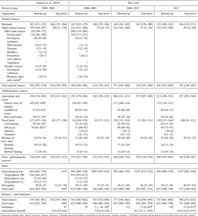
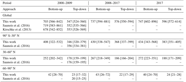
For the 2008–2017 decade, global methane emissions are estimated by atmospheric inversions (a top-down approach) to be 576 Tg CH4yr−1(range 550–594, corresponding to the minimum and maximum estimates of the model ensemble). Of this total, 359 Tg CH4yr−1or ∼ 60 % is attributed to anthropogenic sources, that is emis-sions caused by direct human activity (i.e. anthropogenic emisemis-sions; range 336–376 Tg CH4yr−1or 50 %–65 %). The mean annual total emission for the new decade (2008–2017) is 29 Tg CH4yr−1larger than our estimate for the previous decade (2000–2009), and 24 Tg CH4yr−1larger than the one reported in the previous budget for 2003–2012 (Saunois et al., 2016). Since 2012, global CH4emissions have been tracking the warmest scenarios assessed by the Intergovernmental Panel on Climate Change. Bottom-up methods suggest almost 30 % larger global emissions (737 Tg CH4yr−1, range 594–881) than top-down inversion methods. Indeed, bottom-up es-timates for natural sources such as natural wetlands, other inland water systems, and geological sources are higher than top-down estimates. The atmospheric constraints on the top-down budget suggest that at least some of these bottom-up emissions are overestimated. The latitudinal distribution of atmospheric observation-based emissions indicates a predominance of tropical emissions (∼ 65 % of the global budget, < 30◦N) compared to
mid-latitudes (∼ 30 %, 30–60◦N) and high northern latitudes (∼ 4 %, 60–90◦N). The most important source of uncertainty in the methane budget is attributable to natural emissions, especially those from wetlands and other inland waters.
Some of our global source estimates are smaller than those in previously published budgets (Saunois et al., 2016; Kirschke et al., 2013). In particular wetland emissions are about 35 Tg CH4yr−1lower due to improved partition wetlands and other inland waters. Emissions from geological sources and wild animals are also found to be smaller by 7 Tg CH4yr−1by 8 Tg CH4yr−1, respectively. However, the overall discrepancy between bottom-up and top-down estimates has been reduced by only 5 % compared to Saunois et al. (2016), due to a higher estimate of emissions from inland waters, highlighting the need for more detailed research on emissions factors. Priorities for improving the methane budget include (i) a global, high-resolution map of water-saturated soils and inundated areas emitting methane based on a robust classification of different types of emitting habitats; (ii) fur-ther development of process-based models for inland-water emissions; (iii) intensification of methane observa-tions at local scales (e.g., FLUXNET-CH4 measurements) and urban-scale monitoring to constrain bottom-up land surface models, and at regional scales (surface networks and satellites) to constrain atmospheric inversions; (iv) improvements of transport models and the representation of photochemical sinks in top-down inversions; and (v) development of a 3D variational inversion system using isotopic and/or co-emitted species such as ethane to improve source partitioning.
The data presented here can be downloaded from https://doi.org/10.18160/GCP-CH4-2019 (Saunois et al., 2020) and from the Global Carbon Project.
1 Introduction
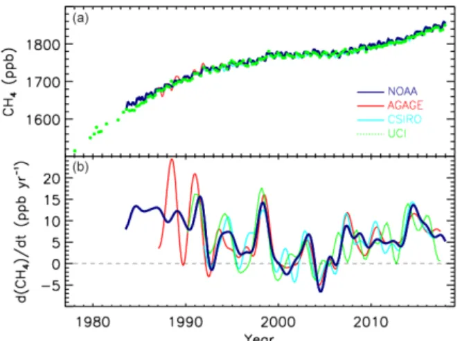
The surface dry air mole fraction of atmospheric methane (CH4) reached 1857 ppb in 2018 (Fig. 1), approximately 2.6 times greater than its estimated pre-industrial equilib-rium value in 1750. This increase is attributable in large part to increased anthropogenic emissions arising primar-ily from agriculture (e.g., livestock production, rice culti-vation, biomass burning), fossil fuel production and use, waste disposal, and alterations to natural methane fluxes due to increased atmospheric CO2 concentrations and cli-mate change (Ciais et al., 2013). Atmospheric CH4 is a stronger absorber of Earth’s emitted thermal infrared radi-ation than carbon dioxide (CO2), as assessed by its global warming potential (GWP) relative to CO2. For a 100-year time horizon and without considering climate feedbacks GWP(CH4) = 28 (IPCC AR5; Myhre et al., 2013). Although global anthropogenic emissions of CH4 are estimated at around 366 Tg CH4yr−1 (Saunois et al., 2016), represent-ing only 3 % of the global CO2 anthropogenic emissions in units of carbon mass flux, the increase in atmospheric CH4concentrations has contributed ∼ 23 % (∼ 0.62 W m−2) to the additional radiative forcing accumulated in the lower atmosphere since 1750 (Etminan et al., 2016). Changes in other chemical compounds (such as nitrogen oxides, NOx, or carbon monoxide, CO) also influence the forcing of at-mospheric CH4 through changes to its atmospheric life-time. From an emission perspective, the total radiative forc-ing attributable to anthropogenic CH4emissions is currently about 0.97 W m−2(Myhre et al., 2013). Emissions of CH4 contribute to the production of ozone, stratospheric water vapour, and CO2 and most importantly affect its own
life-time (Myhre et al., 2013; Shindell et al., 2012). CH4has a short lifetime in the atmosphere (about 9 years for the year 2010; Prather et al., 2012); hence a stabilization or reduction of CH4emissions leads rapidly, in a few decades, to a sta-bilization or reduction of its atmospheric concentration and therefore its radiative forcing. Reducing CH4 emissions is therefore recognized as an effective option for rapid climate change mitigation, especially on decadal timescales (Shin-dell et al., 2012), because of its shorter lifetime than CO2.
Of concern, the current anthropogenic methane emissions trajectory is estimated to lie between the two warmest IPCC-AR5 scenarios (Nisbet et al., 2016, 2019), i.e., RCP8.5 and RCP6.0, corresponding to temperature increases above 3◦C by the end of this century. This trajectory implies that large reductions of methane emissions are needed to meet the 1.5– 2◦C target of the Paris Agreement (Collins et al., 2013; Nis-bet et al., 2019). Moreover, CH4is a precursor of important air pollutants such as ozone, and, as such, its emissions are covered by two international conventions: the United Nations Framework Convention on Climate Change (UNFCCC) and the Convention on Long-Range Transboundary Air Pollution (CLRTAP), another motivation to reduce its emissions.
Changes in the magnitude and temporal variation (annual to inter-annual) in methane sources and sinks over the past decades are characterized by large uncertainties (Kirschke et al., 2013; Saunois et al., 2017; Turner et al., 2019). Also, the decadal budget suggests relative uncertainties (hereafter reported as min–max ranges) of 20 %–35 % for inventories of anthropogenic emissions in specific sectors (e.g., agri-culture, waste, fossil fuels), 50 % for biomass burning and natural wetland emissions, and reaching 100 % or more for other natural sources (e.g. inland waters, geological sources).
Figure 1. Globally averaged atmospheric CH4 (ppb) (a) and its
annual growth rate GATM (ppb yr−1) (b) from four
measure-ment programmes, National Oceanic and Atmospheric Adminis-tration (NOAA), Advanced Global Atmospheric Gases Experiment (AGAGE), Commonwealth Scientific and Industrial Research Or-ganisation (CSIRO), and University of California, Irvine (UCI). De-tailed descriptions of methods are given in the supplementary ma-terial of Kirschke et al. (2013).
The uncertainty in the chemical loss of methane by OH, the predominant sink of atmospheric methane, is estimated around 10 % (Prather et al., 2012) to 15 % (from bottom-up approaches in Saunois et al., 2016). This represents, for the top-down methods, the minimum relative uncertainty as-sociated with global methane emissions, as other methane sinks (atomic oxygen and chlorine oxidations, soil uptake) are much smaller and the atmospheric growth rate is well-defined (Dlugokencky et al., 2009). Globally, the contribu-tion of natural CH4emissions to total emissions can be quan-tified by combining lifetime estimates with reconstructed pre-industrial atmospheric methane concentrations from ice cores (e.g. Ehhalt et al., 2001). Regionally, uncertainties in emissions may reach 40 %–60 % (e.g. for South America, Africa, China, and India; see Saunois et al., 2016).
In order to verify future emission reductions, for exam-ple to help conduct Paris Agreement’s stocktake, sustained and long-term monitoring of the methane cycle is needed to reach more precise estimation of trends, and reduced un-certainties in anthropogenic emissions (Bergamaschi et al., 2018a; Pacala, 2010). Reducing uncertainties in individual methane sources and thus in the overall methane budget is challenging for at least four reasons. Firstly, methane is emit-ted by a variety of processes, including both natural and an-thropogenic sources, point and diffuse sources, and sources associated with three different emission classes (i.e., bio-genic, thermobio-genic, and pyrogenic). These multiple sources and processes require the integration of data from diverse sci-entific communities. The fact that anthropogenic emissions result from unintentional leakage from fossil fuel produc-tion or agriculture further complicates producproduc-tion of
accu-rate bottom-up emission estimates. Secondly, atmospheric methane is removed by chemical reactions in the atmosphere involving radicals (mainly OH) that have very short life-times (typically ∼ 1 s). The spatial and temporal distribu-tions of OH are highly variable. Although OH can be mea-sured locally, calculating global CH4loss through OH mea-surements would require high-resolution OH meamea-surements (typically half an hour to integrate cloud cover and 1 km spatially to consider OH high reactivity and heterogeneity). As a result, such a calculation is currently possible only through modelling. However, simulated OH concentrations from chemistry–climate models still show uncertain spatio-temporal distribution at regional to global scales (Zhao et al., 2019). Thirdly, only the net methane budget (sources minus sinks) is constrained by precise observations of atmospheric growth rates (Dlugokencky et al., 2009), leaving the sum of sources and the sum of sinks more uncertain. One simplifica-tion for CH4compared to CO2is that the oceanic contribu-tion to the global methane budget is small (∼ 1 %–3 %), mak-ing source estimation predominantly a continental problem (USEPA, 2010b). Finally, we lack observations to constrain (1) process models that produce estimates of wetland extent (Kleinen et al., 2012; Stocker et al., 2014) and wetland emis-sions (Melton et al., 2013; Poulter et al., 2017; Wania et al., 2013), (2) other inland water sources (Bastviken et al., 2011; Wik et al., 2016a), (3) inventories of anthropogenic emis-sions (Höglund-Isaksson, 2012, 2017; Janssens-Maenhout et al., 2019; USEPA, 2012), and (4) atmospheric inversions, which aim to estimate methane emissions from global to re-gional scales (Bergamaschi et al., 2013, 2018b; Houweling et al., 2014; Kirschke et al., 2013; Saunois et al., 2016; Spahni et al., 2011; Thompson et al., 2017; Tian et al., 2016).
The global methane budget inferred from atmospheric ob-servations by atmospheric inversions relies on regional con-straints from atmospheric sampling networks, which are rel-atively dense for northern mid-latitudes, with a number of high-precision and high-accuracy surface stations, but are sparser at tropical latitudes and in the Southern Hemisphere (Dlugokencky et al., 2011). Recently the atmospheric obser-vation density has increased in the tropics due to satellite-based platforms that provide column-average methane mix-ing ratios. Despite continuous improvements in the precision and accuracy of space-based measurements (e.g. Buchwitz et al., 2017), systematic errors greater than several parts per bil-lion on total column observations can still limit the usage of such data to constrain surface emissions (Alexe et al., 2015; Bousquet et al., 2018; Chevallier et al., 2017; Locatelli et al., 2015). The development of robust bias corrections on exist-ing data can help overcome this issue (e.g. Inoue et al., 2016) and satellite-based inversions have been suggested to reduce global and regional flux uncertainties compared to surface-based inversions (e.g. Fraser et al., 2013).
The Global Carbon Project (GCP) seeks to develop a complete picture of the carbon cycle by establishing com-mon, consistent scientific knowledge to support policy
de-bate and actions to mitigate greenhouse gas emissions to the atmosphere (https://www.globalcarbonproject.org/, last ac-cess: 24 June 2020). The objective of this paper is to analyse and synthesize the current knowledge of the global methane budget, by gathering results of observations and models in order to better understand and quantify the main robust fea-tures of this budget and its remaining uncertainties and to make recommendations. We combine results from a large en-semble of bottom-up approaches (e.g., process-based models for natural wetlands, data-driven approaches for other natural sources, inventories of anthropogenic emissions and biomass burning, and atmospheric chemistry models) and top-down approaches (including methane atmospheric observing net-works, atmospheric inversions inferring emissions, and sinks from the assimilation of atmospheric observations into mod-els of atmospheric transport and chemistry). The focus of this work is on decadal budgets and on the update of the previ-ous assessment made for the period 2003–2012 to the more recent 2008–2017 decade. More in-depth analysis of trends and year-to-year changes is left to future publications. The regional budget is further discussed in Stavert et al. (2020) and synthetised in Jackson et al., 2020. Our current paper is a living review, published at about 3-year intervals, to pro-vide an update and new synthesis of available observational, statistical, and model data for the overall CH4budget and its individual components.
Kirschke et al. (2013) were the first to conduct a CH4 bud-get synthesis and were followed by Saunois et al. (2016). Kirschke et al. (2013) reported decadal mean CH4emissions and sinks from 1980 to 2009 based on bottom-up and top-down approaches. Saunois et al. (2016) reported methane emissions for three time periods: (1) the last calendar decade (2000–2009), (2) the last available decade (2003–2012), and (3) the last available year (2012) at the time. Here, we up-date reporting methane emissions and sinks for 2000–2009 decade, for the most recent 2008–2017 decade where data are available, and for the year 2017, reducing the time lag between the last reported year and analysis. The methane budget is presented here at global and latitudinal scales, and data can be downloaded from https://doi.org/10.18160/GCP-CH4-2019 (Saunois et al., 2019).
Five sections follow this introduction. Section 2 presents the methodology used in the budget (units, definitions of source categories and regions, data analysis) and discusses the delay between the period of study of the budget and the release date. Section 3 presents the current knowledge about methane sources and sinks based on the ensemble of bottom-up approaches reported here (models, inventories, data-driven approaches). Section 4 reports atmospheric ob-servations and top-down atmospheric inversions gathered for this paper. Section 5, based on Sects. 3 and 4, provides the updated analysis of the global methane budget by comparing bottom-up and top-down estimates and highlighting differ-ences. Finally, Sect. 6 discusses future developments,
miss-ing components, and the most critical remainmiss-ing uncertain-ties based on our update to the global methane budget.
2 Methodology
2.1 Units used
Unless specified, fluxes are expressed in teragrams of CH4 per year (1 Tg CH4yr−1=1012g CH4yr−1), while atmo-spheric concentrations are expressed as dry air mole frac-tions, in parts per billion (ppb), with atmospheric methane annual increases, GATM, expressed in parts per billion per year. In the tables, we present mean values and ranges for the two decades 2000–2009 and 2008–2017, together with results for the most recent available year (2017). Results ob-tained from previous syntheses (i.e. Saunois et al., 2016) are also given for the decade 2000–2009. Following Saunois et al. (2016) and considering that the number of studies is of-ten relatively small for many individual source and sink esti-mates, uncertainties are reported as minimum and maximum values of the available studies, in brackets. In doing so, we acknowledge that we do not consider the uncertainty of the individual estimates, and we express uncertainty as the range of available mean estimates, i.e., differences across measure-ments and methodologies considered. These minimum and maximum values are those presented in Sect. 2.5 and exclude identified outliers.
The CH4emission estimates are provided with up to three digits, for consistency across all budget flux components and to ensure the accuracy of aggregated fluxes. Nonetheless, given the values of the uncertainties in the methane budget, we encourage the reader to consider not more than two digits as significant.
2.2 Period of the budget and availability of data
The bottom-up estimates rely on global anthropogenic inven-tories, land surface models for wetland emissions, and pub-lished literature for other natural sources. The global gridded anthropogenic inventories are updated irregularly, generally every 3 to 5 years. The last reported years of available inven-tories were 2012, 2014, or 2016 when we started this study. For this budget, in order to cover the reported period (2000– 2017), it was necessary to extrapolate some of these datasets as explained in Sect. 3.1.1. The surface land models were run over the full period 2000–2017 using dynamical wetland areas (Sect. 3.2.1).
For the top-down estimates, we use atmospheric inversions covering 2000–2017. The simulations run until mid-2018, but the last year of reported inversion results is 2017, which represents a 3-year lag with the present, a 2-year-shorter lag than for the last release (Saunois et al., 2016). Satellite obser-vations are linked to operational data chains and are gener-ally available days to weeks after the recording of the spectra. Surface observations can lag from months to years because
of the time for flask analyses and data checks in (mostly) non-operational chains. The final 6 months of inversions are generally ignored (spin down) because the estimated fluxes are not constrained by as many observations as the previous periods.
2.3 Definition of regions
Geographically, emissions are reported globally and for three latitudinal bands (90◦S–30◦N, 30–60◦N, 60–90◦N, only for gridded products). When extrapolating emission estimates forward in time (see Sect. 3.1.1), and for the regional budget presented by Stavert et al. (2020), a set of 19 regions (oceans and 18 continental regions; see Fig. S1 in the Supplement) were used. As anthropogenic emissions are often reported by country, we define these regions based on a country list (Table S1). This approach was compatible with all top-down and bottom-up approaches considered. The number of re-gions was chosen to be close to the widely used TransCom inter-comparison map (Gurney et al., 2004) but with subdi-visions to separate the contribution from important countries or regions for the methane cycle (China, South Asia, tropical America, tropical Africa, the United States, and Russia). The resulting region definition is the same as used for the GCP N2O budget (Tian et al., 2019).
2.4 Definition of source categories
Methane is emitted by different processes (i.e., biogenic, thermogenic, or pyrogenic) and can be of anthropogenic or natural origin. Biogenic methane is the final product of the decomposition of organic matter by methanogenic Archaea in anaerobic environments, such as water-saturated soils, swamps, rice paddies, marine sediments, landfills, sewage and wastewater treatment facilities, or inside animal diges-tive systems. Thermogenic methane is formed on geological timescales by the breakdown of buried organic matter due to heat and pressure deep in the Earth’s crust. Thermogenic methane reaches the atmosphere through marine and land ge-ological gas seeps. These methane emissions are increased by human activities, for instance the exploitation and distri-bution of fossil fuels. Pyrogenic methane is produced by the incomplete combustion of biomass and other organic mate-rial. Peat fires, biomass burning in deforested or degraded areas, wildfires, and biofuel burning are the largest sources of pyrogenic methane. Methane hydrates, ice-like cages of trapped methane found in continental shelves and slopes and below sub-sea and land permafrost, can be of either biogenic or thermogenic origin. Each of these three process categories has both anthropogenic and natural components.
In the following, we present the different methane sources depending on their anthropogenic or natural origin, which is relevant for climate policy. Here, “natural sources” re-fer to pre-agricultural emissions even if they are per-turbed by anthropogenic climate change, and “anthropogenic
sources” are caused by direct human activities since pre-industrial/pre-agricultural time (3000–2000 BCE; Nakazawa et al., 1993) including agriculture, waste management, and fossil-fuel-related activities. Natural emissions are split be-tween “wetland” and “other natural” emissions (e.g., non-wetland inland waters, wild animals, termites, land geologi-cal sources, oceanic geologigeologi-cal and biogenic sources, and ter-restrial permafrost). Anthropogenic emissions contain “agri-culture and waste emissions”, “fossil fuel emissions”, and “biomass and biofuel burning emissions”, assuming that all types of fires cause anthropogenic sources, although they are partly of natural origin (Fig. 6; see also Tables 3 and 6).
Our definition of natural and anthropogenic sources does not correspond exactly to the definition used by the UN-FCCC following the IPCC guidelines (IPCC, 2006), where, for pragmatic reasons, all emissions from managed land are reported as anthropogenic, which is not the case here. For instance, we consider all wetlands to be natural sions, despite some wetlands being managed and their emis-sions being partly reported in UNFCCC national communi-cations. The human-induced perturbation of climate, atmo-spheric CO2, and nitrogen and sulfur deposition may cause changes in the sources we classified as natural. Following our definition, emissions from wetlands, inland water, or thawing permafrost will be accountable in natural emissions, even though we acknowledge that climate change – a human perturbation – may cause increasing emissions from these sources. Methane emissions from reservoirs are considered natural even though reservoirs are human-made, and since the 2019 refinement to the IPCC guidelines (IPCC, 2006, 2019) emissions from reservoirs and other flooded lands are considered anthropogenic by the UNFCCC.
Following Saunois et al. (2016), we report anthropogenic and natural methane emissions for five main source cate-gories for both bottom-up and top-down approaches.
Bottom-up estimates of methane emissions for some pro-cesses are derived from process-oriented models (e.g., bio-geochemical models for wetlands, models for termites), in-ventory models (agriculture and waste emissions, fossil fuel emissions, biomass and biofuel burning emissions), satellite-based models (large scale biomass burning), or observation-based upscaling models for other sources (e.g., inland wa-ter, geological sources). From these bottom-up approaches, it is possible to provide estimates for more detailed source subcategories inside each main GCP category (see budget in Table 3). However, the total methane emission derived from the sum of independent bottom-up estimates remains uncon-strained.
For atmospheric inversions (top-down approach) the situ-ation is different. Atmospheric observsitu-ations provide a con-straint on the global total source and a reasonable concon-straint on the global sink derived from methyl chloroform (Montzka et al., 2011; Rigby et al., 2017). The inversions reported in this work solve either for a total methane flux (e.g. Pison et al., 2013) or for a limited number of source categories (e.g.
Bergamaschi et al., 2013). In most of the inverse systems the atmospheric oxidant concentrations are prescribed with pre-optimized or scaled OH fields, and thus the atmospheric sink is not solved. The assimilation of CH4observations alone, as reported in this synthesis, can help to separate sources with different locations or temporal variations but cannot fully separate individual sources as they often overlap in space and time in some regions. Top-down global and regional methane emissions per source category were obtained directly from gridded optimized fluxes, wherever an inversion had solved for the separate five main GCP categories. Alternatively, if an inversion only solved for total emissions (or for categories other than the main five described above), then the prior con-tribution of each source category at the spatial resolution of the inversion was scaled by the ratio of the total (or embed-ding category) optimized flux divided by the total (or em-bedding category) prior flux (Kirschke et al., 2013). In other words, the prior relative mix of sources at model resolution is kept while updating total emissions with atmospheric ob-servations. The soil uptake was provided separately in order to report total gross surface emissions instead of net fluxes (sources minus soil uptake).
In summary, bottom-up models and inventories are pre-sented for all source processes and for the five main cate-gories defined above globally. Top-down inversions are re-ported globally and only for the five main emission cate-gories.
2.5 Processing of emission maps and box-plot
representation of emission budgets
Common data analysis procedures have been applied to the different bottom-up models, inventories, and atmospheric in-versions whenever gridded products exist. Gridded emissions from atmospheric inversions and land surface models for wetland or biomass burning were provided at the monthly scale. Emissions from anthropogenic inventories are usually available as yearly estimates. These monthly or yearly fluxes were provided on a 1◦×1◦grid or re-gridded to 1◦×1◦, then converted into units of teragrams of methane per grid cell. In-versions with a resolution coarser than 1◦were downscaled to 1◦by each modelling group. Land fluxes in coastal pixels were reallocated to the neighbouring land pixel according to our 1◦land–sea mask, and vice versa for ocean fluxes. An-nual and decadal means used for this study were computed from the monthly or yearly gridded 1◦×1◦maps.
Budgets are presented as box plots with quartiles (25 %, median, 75 %), outliers, and minimum and maximum values without outliers. Outliers were determined as values below the first quartile minus 3 times the inter-quartile range, or values above the third quartile plus 3 times the inter-quartile range. Mean values reported in the tables are represented as “+” symbols in the corresponding figures.
3 Methane sources and sinks: bottom-up estimates
For each source category, a short description of the relevant processes, original datasets (measurements, models), and re-lated methodology is given. More detailed information can be found in original publication references and in the Sup-plement of this study.
3.1 Anthropogenic sources
3.1.1 Global inventories gathered
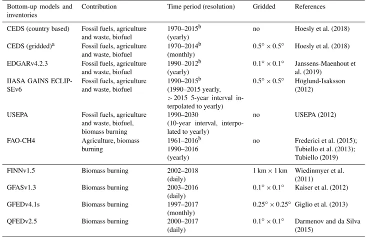
The main bottom-up global inventory datasets covering an-thropogenic emissions from all sectors (Table 1) are from the United States Environmental Protection Agency (USEPA, 2012), the Greenhouse gas and Air pollutant Interactions and Synergies (GAINS) model developed by the International Institute for Applied Systems Analysis (IIASA) (Gomez Sanabria et al., 2018; Höglund-Isaksson, 2012, 2017), and the Emissions Database for Global Atmospheric Research (EDGARv3.2.2; Janssens-Maenhout et al., 2019) compiled by the European Commission Joint Research Centre (EC-JRC) and Netherland’s Environmental Assessment Agency (PBL). We also used the Community Emissions Data System for historical emissions (CEDS) (Hoesly et al., 2018) devel-oped for climate modelling and the Food and Agriculture Or-ganization (FAO) dataset emission database (Tubiello, 2019), which only covers emissions from agriculture and land use (including peatland and biomass fires).
These inventory datasets report emissions from fossil fuel production, transmission, and distribution; livestock enteric fermentation; manure management and application; rice cul-tivation; solid waste; and wastewater. Since the level of detail provided by country and by sector varies among inventories, the data were reconciled into common categories according to Table S2. For example, agricultural and waste burning emissions treated as a separate category in EDGAR, GAINS, and FAO are included in the biofuel sector in the USEPA in-ventory and in the agricultural sector in CEDS. The GAINS, EDGAR, and FAO estimates of agricultural waste burning were excluded from this analysis (these amounted to 1– 3 Tg CH4yr−1) in recent decades to prevent any inadvertent overlap with separate estimates of biomass burning sions (e.g. GFEDv4.1s). In the inventories used here, emis-sions for a given region/country and a given sector are usu-ally calculated following IPCC methodology (IPCC, 2006), as the product of an activity factor and an emission factor for this activity. An abatement coefficient is used addition-ally, to account for any regulations implemented to control emissions (see e.g. Höglund-Isaksson et al., 2015). These datasets differ in their assumptions and data used for the cal-culation; however, they are not completely independent be-cause they follow the same IPCC guidelines (IPCC, 2006), and, at least for agriculture, use the same FAOSTAT ac-tivity data. While the USEPA inventory adopts emissions
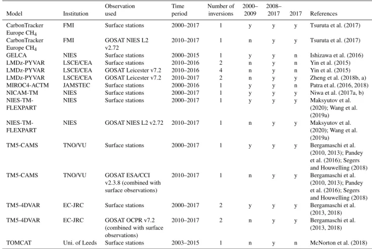
Table 1.Bottom-up models and inventories for anthropogenic and biomass burning estimates used in this study.aDue to its limited sectorial breakdown this dataset was used in Table 3 for the main categories only, replacing CEDS country-based estimates.bExtended to 2017 for this study as described in Sect. 3.1.1.
Bottom-up models and inventories
Contribution Time period (resolution) Gridded References
CEDS (country based) Fossil fuels, agriculture and waste, biofuel
1970–2015b (yearly)
no Hoesly et al. (2018) CEDS (gridded)a Fossil fuels, agriculture
and waste, biofuel
1970–2014b (monthly)
0.5◦×0.5◦ Hoesly et al. (2018) EDGARv4.2.3 Fossil fuels, agriculture
and waste, biofuel
1990–2012b (yearly)
0.1◦×0.1◦ Janssens-Maenhout et al. (2019)
IIASA GAINS ECLIP-SEv6
Fossil fuels, agriculture and waste, biofuel
1990–2015b (1990–2015 yearly, >2015 5-year interval in-terpolated to yearly)
0.5◦×0.5◦ Höglund-Isaksson (2012)
USEPA Fossil fuels, agriculture and waste, biofuel, biomass burning
1990–2030
(10-year interval, interpo-lated to yearly)
no USEPA (2012)
FAO-CH4 Agriculture, biomass burning 1961–2016b 1990–2016 (yearly) no Frederici et al. (2015); Tubiello et al. (2013); Tubiello (2019) FINNv1.5 Biomass burning 2002–2018
(daily)
1 km × 1 km Wiedinmyer et al. (2011)
GFASv1.3 Biomass burning 2003–2016 (daily)
0.1◦×0.1◦ Kaiser et al. (2012) GFEDv4.1s Biomass burning 1997–2017
(monthly)
0.25◦×0.25◦ Giglio et al. (2013) QFEDv2.5 Biomass burning 2000–2017
(daily)
0.1◦×0.1◦ Darmenov and da Silva (2015)
reported by the countries to the UNFCCC, other invento-ries (FAOSTAT, EDGAR, and the GAINS model) produce their own estimates using a consistent approach for all coun-tries. These other inventories compile country-specific ac-tivity data and emission factor information or, if not avail-able, adopt IPCC default factors (Höglund-Isaksson, 2012; Janssens-Maenhout et al., 2019; Tubiello, 2019). The CEDS takes a different approach starting from pre-existing default emission estimates; for methane, a combination of EDGAR and FAO estimates is used, scaled to match other individual or region-specific inventory values when available. This pro-cess maintains the spatial information in the default emission inventories while preserving consistency with country-level data. The FAOSTAT dataset (hereafter FAO-CH4) was used to provide estimates of methane emissions at the country level but is limited to agriculture (enteric fermentation, ma-nure management, rice cultivation, energy usage, burning of crop residues, and prescribed burning of savannahs) and land use (biomass burning). FAO-CH4 uses activity data mainly from the FAOSTAT crop and livestock production database, as reported by countries to the FAO (Tubiello et al., 2013), and applies mostly the Tier 1 IPCC methodology for emis-sions factors (IPCC, 2006), which depend on geographic
lo-cation and development status of the country. For manure, the necessary country-scale temperature was obtained from the FAO global agroecological zone database (GAEZv3.0, 2012). Although country emissions are reported annually to the UNFCCC by Annex I countries, and episodically by non-Annex I countries, data gaps of those national inventories do not allow the inclusion of these estimates in this analysis.
In this budget, we use the following versions of these databases (see Table 1):
– EDGARv4.3.2, which provides yearly gridded emis-sions by sectors from 1970 to 2012 (Janssens-Maenhout et al., 2019);
– GAINS model scenario ECLIPSE v6 (Gomez Sanabria et al., 2018; Höglund-Isaksson, 2012, 2017), which pro-vides both annual sectoral totals by country from 1990 to 2015 and a projection for 2020 (that assumes current emission legislation for the future) and an annual secto-rial gridded product from 1990 to 2015;
– USEPA (USEPA, 2012), which provides 5-year secto-rial totals by country from 1990 to 2020 (estimates from 2005 onward are a projection), with no gridded distribu-tion available;
– CEDS version 2017-05-18, which provides both grid-ded monthly and annual country-based emissions by sectors from 1970 to 2014 (Hoesly et al., 2018); – FAO-CH4 (database accessed in February 2019, FAO,
2019) containing annual country-level data for the pe-riod 1961–2016, for rice, manure, and enteric fermenta-tion and 1990–2016 for burning savannah, crop residue, and non-agricultural biomass burning.
In order to report emissions for the period 2000–2017, we extended and interpolated some of the datasets as ex-plained in Sect. 2.2. The USEPA dataset was linearly in-terpolated to provide yearly values. The FAO-CH4 dataset, ending in 2016, was extrapolated to 2017 using a linear fit based on 2014–2016 data. EDGARv4.3.2 was extrapo-lated to 2017 using the extended FAO-CH4 emissions for enteric fermentation, manure management, and rice cultiva-tion and using the BP statistical review of fossil fuel pro-duction and consumption (BP Statistical Review of World Energy, 2019) for emissions from the coal, oil, and gas sec-tors. In this extrapolated inventory, called EDGARv4.3.2EXT, methane emissions for year t are set equal to the 2012 (last year) EDGAR emissions (EEDGARv4.3.2) times the ra-tio between FAO-CH4 emissions (or BP statistics) of year t (EFAO-CH4(t )) and FAO-CH4 emissions (or BP statistics) of 2012 (EFAO-CH4(2012)). For each emission sector, region-specific emissions of EDGARv4.3.2EXT in year t are esti-mated following Eq. (1):
EEDGARv4.3.2ext(t ) =
EEDGARv4.3.2(2012) × EFAO-CH4(t )/EFAO-CH4(2012). (1) Transport, industrial, waste, and biofuel sources were lin-early extrapolated in EDGARv4.3.2EXT based on the last 3 years of data while other sources were kept constant at the 2012 level. To allow comparisons through 2017, the CEDS dataset has also been extrapolated in an identical method cre-ating CEDSEXT. However, in contrast to the EDGARv4.3.2 dataset, the CEDS dataset provides only a combined oil and gas sector; hence, we extended this sector using the sum of BP oil and gas emissions. The by-country GAINS dataset was linearly projected by sector for each country using the trend between the historical 2015 and projected 2020 val-ues. These by-country projections were aggregated to the 19 global regions (Sect. 2.3 and Fig. S1) and used to extrapo-late the GAINS gridded dataset in a similar manner to that described in Eq. (1). Although we only use the extended in-ventories, in the following the “EXT” suffix will be dropped for clarity.
3.1.2 Total anthropogenic emissions
In order to avoid double-counting and ensure consistency with each inventory, the range (min–max) and mean values of the total anthropogenic emissions were not calculated as the
sum of the mean and range of the three anthropogenic cate-gories (“agriculture and waste”, “fossil fuels”, and “biomass burning & biofuels”). Instead, we calculated separately the total anthropogenic emissions for each inventory by adding its values for agriculture and waste, fossil fuels, and biofuels with the range of available large-scale biomass burning emis-sions. This approach was used for the EGDARv4.3.2, CEDS, and GAINS inventories, but we kept the USEPA inventory as originally reported because it includes its own estimates of biomass burning emissions. FAO-CH4was only included in the range reported for the agriculture and waste category. For the latter, we calculated the range and mean value as the sum of the mean and range of the three anthropogenic subcat-egory estimates “enteric fermentation and manure”, “rice”, and “landfills and waste”. The values reported for the upper-level anthropogenic categories (agriculture and waste, fossil fuels, and biomass burning & biofuels) are therefore consis-tent with the sum of their subcategories, although there might be small percentage differences between the reported total anthropogenic emissions and the sum of the three upper-level categories. This approach provides a more accurate represen-tation of the range of emission estimates, avoiding an artifi-cial expansion of the uncertainty attributable to subtle differ-ences in the definition of sub-sector categorizations between inventories.
Based on the ensemble of databases detailed above, total anthropogenic emissions were 366 [349–393] Tg CH4yr−1 for the decade 2008–2017 (Table 3, including biomass and biofuel burning) and 334 [321–358] Tg CH4yr−1 for the decade 2000–2009. Our estimate for the preceding decade is statistically consistent with Saunois et al. (2016) (338 Tg CH4yr−1 [329–342]) and Kirschke et al. (2013) (331 Tg CH4yr−1 [304–368]) for the same period. The slightly larger range reported herein with respect to previ-ous estimates is mainly due to a larger range in the biomass burning estimates, as more biomass burning products are in-cluded in this update. The range associated with our esti-mates (∼ 10 %–12 %) is smaller than the range reported in Höglund-Isaksson et al. (2015) (∼ 20 %), perhaps because they analysed data from a wider range of inventories and projections, plus this study was referenced to one year only (2005) rather than averaged over a decade, as done here.
Figure 2a summarizes global methane emissions of an-thropogenic sources (including biomass and biofuel burn-ing) by different datasets between 2000 and 2050. The datasets consistently estimate total anthropogenic emissions of ∼ 300 Tg CH4yr−1 in 2000. The main discrepancy be-tween the inventories is their trend after 2005, with the lowest emissions projected by GAINS and the largest by CEDS. With the U.S. EPA being a projection from 2005 onward, its values and trends deviate from others. For the Sixth Assessment report of the IPCC, seven main Shared Socioeconomic Pathways (SSPs) were defined for future climate projections in the Coupled Model Intercomparison Project Phase 6 (CMIP6) (Gidden et al., 2019; O’Neill et
Figure 2.(a, b) Global anthropogenic methane emissions (including biomass burning) from historical inventories and future projections (Tg CH4yr−1). (a) Inventories and the unharmonized Shared Socioeconomic Pathways (Riahi et al., 2017), with highlighted scenarios
representing scenarios assessed in CMIP6 (O’Neill, et al., 2016). (b) The selected scenarios harmonized with historical emissions (CEDS) for CMIP6 activities (Gidden et al., 2019). USEPA and GAINS estimates have been linearly interpolated from the 5-year original products to yearly values. After 2005, USEPA original estimates are projections. (c) Global methane concentrations for NOAA surface site observations (black) and projections based on SSPs (Riahi et al., 2017) with concentrations estimated using MAGICC (Meinshausen et al., 2011).
al., 2016) ranging from 1.9 to 8.5 W m−2 radiative forc-ing by the year 2100 (as shown by the number in the SSP names). The trends in methane emissions from 2010 esti-mated by current inventories track the pathways with the highest radiative forcing in 2100 (based on the unharmo-nized scenarios developed by integrated assessment models, Fig. 2a). For the 1970–2015 period, historical emissions used in CMIP6 (Feng et al., 2019) combine anthropogenic emis-sions from CEDS (Hoesly et al., 2018) and a climatological value from the GFEDv4.1s biomass burning inventory (van Marle et al., 2017). The CEDS anthropogenic emissions es-timates, based on EDGARv4.2, are 10–20 Tg higher than the more recent EDGARv4.3.2 (van Marle et al., 2017). Har-monized scenarios used for CMIP6 activities start in 2015 at 388 Tg CH4yr−1. Since methane emissions continue to track scenarios that assume no or minimal climate policies,
it may indicate that climate policies, when present, have not yet produced sufficient results to change the emissions tra-jectory substantially (Nisbet et al., 2019). After 2015, the SSPs span a range of possible outcomes, but current emis-sions appear likely to follow the higher-emission trajectories over the next decade (Fig. 2b). This illustrates the challenge of methane mitigation that lies ahead to help reach the goals of the Paris Agreement. In addition, estimates of methane atmospheric concentrations from the unharmonized scenar-ios (Riahi et al., 2017) indicate that observations of global methane concentrations fall well within the range of scenar-ios (Fig. 2c). The methane concentrations are estimated using a simple exponential decay with inferred natural emissions (Meinshausen et al., 2011), and the emergence of any trend between observations and scenarios needs to be confirmed in the following years. In the future, it will be important to
monitor the trends from the year 2015 (the Paris Agreement) estimated in inventories and from atmospheric observations and compare them to various scenarios.
3.1.3 Fossil fuel production and use
Most anthropogenic methane emissions related to fossil fu-els come from the exploitation, transportation, and usage of coal, oil, and natural gas. Additional emissions reported in this category include small industrial contributions such as production of chemicals and metals, fossil fuel fires (e.g., un-derground coal mine fires and the Kuwait oil and gas fires), and transport (road and non-road transport). Methane emis-sions from the oil industry (e.g. refining) and production of charcoal are estimated to be a few teragrams of methane per year only and are included in the transformation industry sec-tor in the invensec-tory. Fossil fuel fires are included in the sub-category “oil & gas”. Emissions from industries and road and non-road transport are reported apart from the two main sub-categories oil & gas and “coal mining”, contrary to Saunois et al. (2016); each of these amounts to about 5 Tg CH4yr−1 (Table 3). The large range (0–12 Tg CH4yr−1) is attributable to difficulties in allocating some sectors to these sub-sectors consistently among the different inventories (see Table S2). The spatial distribution of methane emissions from fossil fuels is presented in Fig. 3 based on the mean gridded maps provided by CEDS, EDGARv4.3.2, and GAINS for the 2008–2017 decade; the USEPA lacks a gridded product.
Global mean emissions from fossil-fuel-related activi-ties, other industries, and transport are estimated from the four global inventories (Table 1) to be of 128 [113– 154] Tg CH4yr−1 for the 2008–2017 decade (Table 3), but with large differences in the rate of change during this period across inventories. The sector accounts on average for 35 % (range 30 %–42 %) of total global anthropogenic emissions.
Coal mining
During mining, methane is emitted primarily from ventila-tion shafts, where large volumes of air are pumped into the mine to keep the CH4mixing ratio below 0.5 % to avoid acci-dental ignition, and from dewatering operations. In countries of the Organization for Economic Co-operation and Devel-opment (OECD), methane released from ventilation shafts is in principle used as fuel, but in many countries, it is still emitted into the atmosphere or flared, despite the ef-forts for coal mine recovery under the UNFCCC Clean De-velopment Mechanisms (http://cdm.unfccc.int, last access: 29 June 2020). Methane also leaks occur during post-mining handling, processing, and transportation. Some CH4 is re-leased from coal waste piles and abandoned mines; while emissions from these sources were believed to be low (IPCC, 2000), recent work has estimated these to be 22 billion m3 (compared with 103 billion m3from functioning coal mines)
in 2010 with emissions projected to increase into the future (Kholod et al., 2020).
In 2017, almost 40 % (IEA, 2019b) of the world’s electric-ity was still produced from coal. This contribution grew in the 2000s at the rate of several per cent per year, driven by Asian economic growth where large reserves exist, but global coal consumption has declined since 2014. In 2018, the top 10 largest coal producing nations accounted for ∼ 90 % of total world methane emissions for coal mining; among them, the top three producers (China, United States, and India) pro-duced almost two-thirds (64 %) of the world’s coal (IEA, 2019a).
Global estimates of CH4emissions from coal mining show a large range of 29–61 Tg CH4yr−1 for 2008–2017, in part due to the lack of comprehensive data from all major produc-ing countries. The highest value of the range comes from the CEDS inventory while the lowest comes from the USEPA. CEDS seems to have overestimated coal mining emissions from China by almost a factor of 2, most likely due to its de-pendence on the EDGARv4.2 emission inventory. As high-lighted by Saunois et al. (2016), a county-based inventory of Chinese methane emissions also confirms the overestimate of about +38 % with total anthropogenic emissions estimated at 43 ± 6 Tg CH4yr−1(Peng et al., 2016). The EDGARv4.2 inventory follows the IPCC guidelines and uses a European averaged emission factor for CH4 from coal production to substitute missing data for China, which appear to be over-estimated by a factor of approximately 2. These differences highlight significant errors resulting from the use of emission factors, and applying Tier 1 approaches for coal mine emis-sions is not sufficiently accurate as stated by the IPCC guide-lines. The newly released version of EDGARv4.3.2 used here has revised China coal methane emission factors downwards and distributed them to more than 80 times more coal min-ing locations in China. Coal minmin-ing emission factors depend strongly on the type of coal extraction (underground min-ing emits up to 10 times more than surface minmin-ing), geolog-ical underground structure (region-specific), history (basin uplift), and quality of the coal (brown coal emits more than hard coal). Finally, coal mining is the main source explaining the differences between inventories globally (Fig. 2).
For the 2008–2017 decade, methane emissions from coal mining represent 33 % of total fossil-fuel-related emissions of methane (42 Tg CH4yr−1, range of 29–61). An addi-tional very small source corresponds to fossil fuel fires (mostly underground coal fires, ∼ 0.15 Tg yr−1 in 2012, EDGARv4.3.2).
Oil and natural gas systems
This subcategory includes emissions from both conventional and shale oil and gas exploitation. Natural gas is comprised primarily of methane, so both fugitive and planned emissions during the drilling of wells in gas fields, extraction, trans-portation, storage, gas distribution, end use, and incomplete
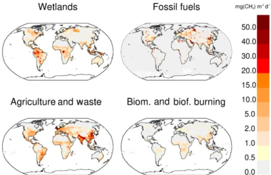
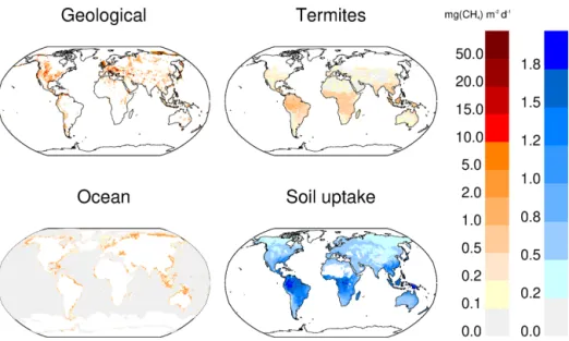
Figure 3.Methane emissions from four source categories: natural wetlands (excluding lakes, ponds, and rivers), biomass and biofuel burning, agriculture and waste, and fossil fuels for the 2008–2017 decade (mg CH4m−2d−1). The wetland emission map represents the mean daily
emission average over the 13 biogeochemical models listed in Table 2 and over the 2008–2017 decade. Fossil fuel and agriculture and waste emission maps are derived from the mean estimates of gridded CEDS, EGDARv4.3.2, and GAINS models. The biomass and biofuel burning map results from the mean of the biomass burning inventories listed in Table 1 added to the mean of the biofuel estimate from CEDS, EDGARv4.3.2, and GAINS models.
combustion of gas flares emit methane (Lamb et al., 2015; Shorter et al., 1996). Persistent fugitive emissions (e.g., due to leaky valves and compressors) should be distinguished from intermittent emissions due to maintenance (e.g. purg-ing and drainpurg-ing of pipes). Durpurg-ing transportation, fugitive emissions can occur in oil tankers, fuel trucks, and gas trans-mission pipelines, attributable to corrosion, manufacturing, and welding faults. According to Lelieveld et al. (2005), CH4 fugitive emissions from gas pipelines should be rel-atively low; however distribution networks in older cities may have higher rates, especially those with cast-iron and unprotected steel pipelines (Phillips et al., 2013). Measure-ment campaigns in cities within the United States and Eu-rope revealed that significant emissions occur in specific lo-cations (e.g. storage facilities, city gates, well and pipeline pressurization–depressurization points) along the distribu-tion networks (e.g. Jackson et al., 2014a; McKain et al., 2015; Wunch et al., 2016). However, methane emissions vary significantly from one city to another depending, in part, on the age of city infrastructure and the quality of its mainte-nance, making urban emissions difficult to scale up. In many facilities, such as gas and oil fields, refineries, and offshore platforms, venting of natural gas is now replaced by flar-ing with almost complete conversion to CO2; these two pro-cesses are usually considered together in inventories of oil and gas industries. Also, single-point failure of natural gas infrastructure can leak methane at a high rate for months, such as at the Aliso Canyon blowout in the Los Angeles,
CA, basin (Conley et al., 2016) or the recent shale gas well blowout in Ohio (Pandey et al., 2019), thus hampering emis-sion control strategies. Production of natural gas from the exploitation of hitherto unproductive rock formations, espe-cially shale, began in the 1970s in the United States on an experimental or small-scale basis, and then, from the early 2000s, exploitation started at large commercial scale. The shale gas contribution to total dry natural gas production in the United States reached 62 % in 2017, growing rapidly from 40 % in 2012, with only small volumes produced be-fore 2005 (EIA, 2019). The possibly larger emission fac-tors from the shale gas compared to the conventional ones have been widely debated (e.g. Cathles et al., 2012; Howarth, 2019; Lewan, 2020). However, the latest studies tend to infer similar emission factors in a narrow range of 1 %–3 % (Al-varez et al., 2018; Peischl et al., 2015; Zavala-Araiza et al., 2015), different from the widely spread rates of 3 %–17 % from previous studies (e.g. Caulton et al., 2014; Schneising et al., 2014).
Methane emissions from oil and natural gas systems vary greatly in different global inventories (72 to 97 Tg yr−1 in 2017, Table 3). The inventories generally rely on the same sources and magnitudes for activity data, with the de-rived differences therefore resulting primarily from different methodologies and parameters used, including emission fac-tors. Those factors are country- or even site-specific, and the few field measurements available often combine oil and gas activities (Brandt et al., 2014) and remain largely unknown
for most major oil- and gas-producing countries. Depend-ing on the country, the reported emission factors may vary by 2 orders of magnitude for oil production and by 1 order of magnitude for gas production (Table S5.1 of Höglund-Isaksson, 2017). The GAINS estimate of methane emis-sions from oil production, for instance, is twice as high as EDGARv4.3.2. For natural gas, the uncertainty is of a sim-ilar order of magnitude. During oil extraction, natural gas generated can be either recovered (re-injected or utilized as an energy source) or not recovered (flared or vented to the atmosphere). The recovery rates vary from one country to another (being much higher in the United States, Europe, and Canada than elsewhere) and from one type of oil to an-other: flaring is less common for heavy oil wells than for con-ventional ones (Höglund-Isaksson et al., 2015). Considering recovery rates could lead to 2-times-higher methane emis-sions accounting for country-specific rates of generation and recovery of associated gas than when using default values (Höglund-Isaksson, 2012). This difference in methodology explains, in part, why GAINS estimates are higher than those of EDGARv4.3.2.
Most studies (Alvarez et al., 2018; Brandt et al., 2014; Jackson et al., 2014b; Karion et al., 2013; Moore et al., 2014; Olivier and Janssens-Maenhout, 2014; Pétron et al., 2014; Zavala-Araiza et al., 2015), albeit not all (Allen et al., 2013; Cathles et al., 2012; Peischl et al., 2015), sug-gest that methane emissions from oil and gas industry are underestimated by inventories and agencies, including the USEPA. Zavala-Araiza et al. (2015) showed that a few high-emitting facilities, i.e., super-emitters, neglected in the inven-tories, dominated US emissions. These high-emitting points, located on the conventional part of the facility, could be avoided through better operating conditions and repair of malfunctions. As US production increases, absolute methane emissions almost certainly increase. US crude oil production also doubled over the last decade and natural gas production rose more than 50 % (EIA, 2019). However, global implica-tions of the rapidly growing shale gas activity in the United States remain to be determined precisely.
For the 2008–2017 decade, methane emissions from up-stream and downup-stream oil and natural gas sectors are esti-mated to represent about 63 % of total fossil CH4emissions (80 Tg CH4yr−1, range of 68–92 Tg CH4yr−1, Table 3), with a lower uncertainty range than for coal emissions for most countries.
3.1.4 Agriculture and waste sectors
This main category includes methane emissions related to livestock production (i.e., enteric fermentation in ruminant animals and manure management), rice cultivation, landfills, and wastewater handling. Of these, globally and in most countries, livestock is by far the largest source of CH4, fol-lowed by waste handling and rice cultivation. Conversely, field burning of agricultural residues is a minor source of
CH4 reported in emission inventories. The spatial distribu-tion of methane emissions from agriculture and waste han-dling is presented in Fig. 3 based on the mean gridded maps provided by CEDS, EDGARv4.3.2, and GAINS over the 2008–2017 decade.
Global emissions from agriculture and waste for the pe-riod 2008–2017 are estimated to be 206 Tg CH4yr−1(range 191–223, Table 3), representing 56 % of total anthropogenic emissions.
Livestock: enteric fermentation and manure management
Domestic ruminants such as cattle, buffalo, sheep, goats, and camels emit methane as a by-product of the anaerobic micro-bial activity in their digestive systems (Johnson et al., 2002). The very stable temperatures (about 39◦C) and pH (6.5–6.8) values within the rumen of domestic ruminants, along with a constant plant matter flow from grazing (cattle graze many hours per day), allow methanogenic Archaea residing within the rumen to produce methane. Methane is released from the rumen mainly through the mouth of multi-stomached rumi-nants (eructation, ∼ 87 % of emissions) or absorbed in the blood system. The methane produced in the intestines and partially transmitted through the rectum is only ∼ 13 %.
The total number of livestock continues to grow steadily. There are currently (2017) about 1.5 billion cattle globally, 1 billion sheep, and nearly as many goats (http://www.fao.org/ faostat/en/#data/GE, last access: 29 June 2020). Livestock numbers are linearly related to CH4 emissions in invento-ries using the Tier 1 IPCC approach such as FAOSTAT. In practice, some non-linearity may arise due to dependencies of emissions on total weight of the animals and their diet, which are better captured by Tier 2 and higher approaches. Cattle, due to their large population, large individual size, and particular digestive characteristics, account for the majority of enteric fermentation CH4emissions from livestock world-wide (Tubiello, 2019), particularly in intensive agricultural systems in wealthier and emerging economies, including the United States (USEPA, 2016). Methane emissions from en-teric fermentation also vary from one country to another as cattle may experience diverse living conditions that vary spa-tially and temporally, especially in the tropics (Chang et al., 2019).
Anaerobic conditions often characterize manure decompo-sition in a variety of manure management systems globally (e.g., liquid/slurry treated in lagoons, ponds, tanks, or pits), with the volatile solids in manure producing CH4. In contrast, when manure is handled as a solid (e.g., in stacks or dry lots) or deposited on pasture, range, or paddock lands, it tends to decompose aerobically and to produce little or no CH4. How-ever aerobic decomposition of manure tends to produce ni-trous oxide (N2O), which has a larger warming impact than CH4. Ambient temperature, moisture, energy contents of the feed, manure composition, and manure storage or residency time affect the amount of CH4produced. Despite these


![[PDF] Cours et exercices pour débuter avec Illustrator CS5 | Cours informatique](data:image/gif;base64,R0lGODlhAQABAIAAAP///wAAACH5BAEAAAAALAAAAAABAAEAAAICRAEAOw==)