Mid-Holocene climate change in Europe: a data-model comparison

(1)

HAL Id: hal-00330716

https://hal.archives-ouvertes.fr/hal-00330716

Submitted on 20 Nov 2006

HAL is a multi-disciplinary open access

archive for the deposit and dissemination of sci-entific research documents, whether they are pub-lished or not. The documents may come from teaching and research institutions in France or abroad, or from public or private research centers.

L’archive ouverte pluridisciplinaire HAL, est destinée au dépôt et à la diffusion de documents scientifiques de niveau recherche, publiés ou non, émanant des établissements d’enseignement et de recherche français ou étrangers, des laboratoires publics ou privés.

Mid-Holocene climate change in Europe: a data-model

comparison

S. Brewer, Joel Guiot, F. Torre

To cite this version:

S. Brewer, Joel Guiot, F. Torre. Mid-Holocene climate change in Europe: a data-model comparison. Climate of the Past Discussions, European Geosciences Union (EGU), 2006, 2 (6), pp.1155-1186. �hal-00330716�

(2)

CPD

2, 1155–1186, 2006 Mid-Holocene climate change in Europe: a data-model comparison S. Brewer et al. Title Page Abstract Introduction Conclusions References Tables Figures ◭ ◮ ◭ ◮ Back Close

Full Screen / Esc

Printer-friendly Version Interactive Discussion

Clim. Past Discuss., 2, 1155–1186, 2006 www.clim-past-discuss.net/2/1155/2006/ © Author(s) 2006. This work is licensed under a Creative Commons License.

Climate of the Past Discussions

Climate of the Past Discussions is the access reviewed discussion forum of Climate of the Past

Mid-Holocene climate change in Europe:

a data-model comparison

S. Brewer1, J. Guiot1, and F. Torre2 1

CEREGE, CNRS/Universit ´e Paul C ´ezanne UMR 6635, BP 80, 13545 Aix-en-Provence cedex 4, France

2

IMEP/Universit ´e Paul C ´ezanne UMR 6635, BP 80, 13545 Aix-en-Provence cedex 4, France Received: 17 October 2006 – Accepted: 1 November 2006 – Published: 20 November 2006 Correspondence to: S. Brewer (brewer@cerege.fr)

(3)

CPD

Full Screen / Esc

Abstract

We present here a comparison between the outputs of a set of 25 climate models run for the mid-Holocene period (6 ka BP) with a set of palaeo-climate reconstructions from over 400 fossil pollen sequences distributed across the European continent. Three cli-mate parameters were available (moisture availability, temperature of the coldest month 5

and growing degree days), which were then grouped together using cluster analysis to provide regions of homogenous climate change. Each model was then investigated to see if it reproduced 1) the same directions of change and 2) the correct location of these regions. A fuzzy logic distance was used to compare the output of the model with the data, which allowed uncertainties from both the model and data to be taken into 10

account. The initial comparison showed that the models were only capable of repro-ducing regions of little climate change, as the data-based reconstructions have a much larger range of changes due to their local nature. A correction for the model standard deviation was then applied to allow the comparison to proceed, and this second test shows that the majority of models simulate all the observed patterns of climatic change, 15

although most do not simulate the observed magnitude of change. The models were then compared by distance to data, and by the amount of correction required. The ma-jority of the models are grouped together both in distance and correction, suggesting that they are becoming more consistent. A test against a set of zero anomalies (no cli-mate change) shows that, whilst the models are unable to reproduce the exact patterns 20

of change, they all produce the correct direction of change for the mid-Holocene.

1 Introduction

In order to test the ability of models to simulate future climate change under changing environmental conditions, such as the atmospheric composition, they must be tested against known climatic datasets. In addition to testing against the current climate, we 25

also wish to know how well they will simulate climate under different forcing conditions. 1156

(4)

CPD

Full Screen / Esc

In the Paleoclimate Modeling Intercomparison project (PMIP) (Joussaume and Taylor, 1995), climatic simulations have been made for two periods, the mid-Holocene (6 ka BP) and the Last Glacial Maximum (LGM). The mid-Holocene period (6000 yr BP) was chosen as a key period for PMIP (Harrison et al., 1998) as it is a simple modelling experiment with a clear forcing (maximum summer insolation and minimum winter in-5

solation). The PMIP project has also focused on the production of datasets of past climate proxies that may be used to test these reconstructions, and a number of well-controlled continental scale datasets now exist (e.g. Wright Jr. et al., 1993; Prentice et al., 2000; Kim and Schneider, 2004).

A number of studies comparing model output and these proxies have been per-10

formed (e.g. Liao et al., 1994; Harrison et al., 1998; Masson et al., 1998; Prentice et al., 1998; Guiot et al., 1999; Joussaume et al., 1999; Bonfils et al., 2004). The first generation PMIP model (PMIP1) runs were tested by Masson et al. (1998) against a set of gridded climate reconstructions for the mid-Holocene in Europe (Cheddadi et al., 1997). The results showed that the majority of models showed an increase in winter 15

temperatures, in agreement with the proxy-based values. In contrast, few models were able to reproduce the observed summer cooling and increase in moisture availability in the south of Europe. As with other precedent studies, this work was based on vi-sual comparison between maps of climatic parameters. Vivi-sual comparisons will work well where the model-data differences are large enough to be easily identified or the 20

resolution of different models is similar, but where the differences are smaller or model resolution more varied, it becomes harder to make an objective assessment (Guiot et al., 1999).

Other studies have used the kappa statistic to compare maps of land cover derived from simulated paleoclimatic values with pollen data (Texier et al., 1997; Harrison et 25

al., 1998). Whilst this provides an objective measure of the difference between two im-ages, it will also be affected by model resolution and is unable to take into account any slight geographical shifts in the simulated climate patterns. For example, a model that is able to simulate an enhancement of the monsoon but in the wrong location should

(5)

CPD

Full Screen / Esc

perform better in such a test than a model that has no enhancement. Further, Bracon-not and Frankignoul (1993) have shown the importance of including both model and data uncertainty in any comparative study, which cannot be included in the classical kappa statistic.

An improved method should therefore take into account these two features: the un-5

certainties of both the proxy-derived variables and model outputs and situations where patterns of climatic change are correctly simulated in the model, but shifted geograph-ically or in time. Uncertainties may be included in data-model comparisons by using a fuzzy-logic approach, in which the values to be compared are defined as a number with a membership function (Guiot et al., 1999). So when comparing the simulated 10

and reconstructed temperature for a given point, the model temperature would be de-fined by the mean temperature change, and the limits of the membership function by the model standard deviation at that point. Similarly, the membership function of the proxy reconstruction may be defined by the mean reconstructed value and the esti-mated reconstruction errors. This method was first used by Guiot et al. (1999) for 15

testing the PMIP1 models. The study showed that the majority of models simulated a change in climate that was closer to the changes observed in the proxy data than a scenario of no change. However, no model was able to simulate the changes in all the parameters used. The method was subsequently modified by Bonfils et al. (2004) by replacing the pixel-to-pixel comparison by an approach based on clusters, allowing 20

a multi-variate comparison to be made on the basis of coherent patterns of climate change, rather than individual points. Applied to the same set of PMIP1 model outputs, the results showed that whilst some models were able to reproduce all clusters, and therefore all the observed patterns of climate change, they concluded that the models were unable to correctly simulate changes in atmospheric circulations as the changes 25

in mid-Holocene vegetation and ocean conditions were not taken into account, and that future studies with coupled models should improve the data-model fit. More re-cently, the method has been adapted for the comparison of long-time series of model simulations for the last 500 years (Brewer et al., 2006). In this last study, time

(6)

CPD

Full Screen / Esc

ries were available from both the model and the proxy data, adding an additional layer of complexity to the comparison, as changes in both space and time were taken into account. The results showed a good fit at low frequencies for one of the fully forced model runs, and allowed the observed changes to be interpreted in terms of changes in atmospheric circulation, notably during the Little Ice Age.

5

We present here an application of the method using output from the new generation of coupled PMIP models (PMIP2) for the mid-Holocene over Europe and a recent set of continental-scale climate reconstructions. The methods used follow those described by Bonfils et al. (2004), with some changes such as the inclusion of model variance in the distance estimations, and tests of the cluster stability. We first describe the clusters 10

obtained and the climatic information contained in each one, and then compare each model to the obtained patterns. As the study includes climate models of varying levels of complexity (atmosphere-only AGCM, coupled ocean-atmosphere OAGCM, coupled ocean-atmosphere-vegetation OAVGCM), we then examine the differences between model type.

15

2 Methods

2.1 Study area

In order to have a relatively high density of proxy sites, the comparison are made using pollen sites and model grid cells covering the western European continent between 15◦West and 50◦ East and between 30◦and 75◦ North.

20

2.2 Proxy data

A data set of palaeo-climate reconstructions from approximately 350 fossil pollen se-quences distributed across the European continent was used, taken from the recent study by Davis et al. (2003). To obtain a representative sample for the mid-Holocene,

(7)

CPD

Full Screen / Esc

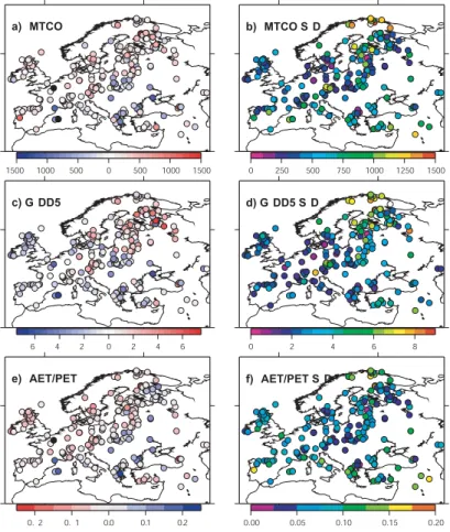
all samples dated to 6 ka BP ± 250 years were selected and then averaged for each site. As the aim of this comparison is to compare climatic changes, 6 ka BP anomalies were calculated by subtracting the reconstructed modern value for each site from the mid-Holocene value. A modern pollen sample was not available for all sites, and the final set of anomalies included 245 sites. We have selected the three bioclimatic pa-5

rameters that are the best reconstructed from fossil pollen assemblages for the com-parison (moisture availability, temperature of the coldest month and growing degree days). The distribution of the sites and the associated anomalies is shown in Fig. 1.

2.3 Models

The study includes output from a total of 25 GCM, comprised of 14 atmosphere-only 10

GCMs, 9 coupled OAGCMs and 2 coupled OAVGCMs. Details of each model and references are given in Table 1.

2.4 K-means cluster analysis

The aim of the cluster analysis is to group together sites showing similar direction and amplitude of climate change. For this we have a matrix consisting of a set of 245 vec-15

tors (one per site) by 3 variables (one per bioclimatic variable). The k-means algorithm was used for the cluster analysis (Hartigan and Wong, 1979). From the dataset, an initial set of k vectors are chosen and the remaining data points are randomly assigned to the closest vector. So k clusters are obtained and their centroid calculated. Then each data point is moved to the closest centroid and a new partition is obtained. This 20

is repeated until a complete pass through all the data points results in no data point moving from one cluster to another. At this point the clusters are considered stable and the clustering process ends.

The number of groups to be obtained is a priori unknown, and the choice is some-what arbitrary. In order to select an optimum number, we use the ratio of inter to 25

intra-group variance of an increasing number of groups, and consider a stopping rule 1160

(8)

CPD

Full Screen / Esc

when the gain was less than 0.05, resulting in the selection of five groups. We then test for the stability of these groups by examining a) if other possible sets of centroids may be obtained; and b) the amount by which the centroids of these groups vary. The k-means algorithm was run 1000 times using a different random start each time, and the standard deviation of the value attributed to the centroid was calculated (Table 2). 5

The standard deviation is relatively high and a closer examination shows that in 20% of the runs, a quite different configuration of groups is obtained, which have a higher intra-group variance. The standard deviation of the centroids obtained from the other 80% of the runs is substantially smaller (Table 2) and we consider that, given that the set of clusters used in the comparison belongs to this dominant solution, they may be 10

considered as stable. The geographical distribution of the selected clusters is shown in Fig. 2. For the comparison, each cluster is represented by its centroid and its extent on each climatic axis and Fig. 3 shows the extent of each cluster in terms of these parameters.

2.5 Hagaman distance 15

A description of the calculation of the Hagaman distance (Bardossy and Duckstein, 1995) used is given in Brewer et al. (2006). Here, we calculate, for each model gridpoint, the Hagaman distance to each of the five selected clusters. For each cli-matic parameter i that used to define the clusters, we obtain two triangular numbers (ri, ri–δri, ri+ηri) and (mi, mi–δmi, mi+ηmi). The first represents the proxy data

clus-20

ter, where is the position of the triangle apex (r_i) is the cluster centroid and the limits

r_i–δri and ri+ηri are defined by the 5th and 95th percentile, respectively. The second

triangular fuzzy number represents the model climate at gridpoint i. The apex (mi) is

the mean model value at that point and the limits m_i–δ_mi and m_i+η

mi are ±2 standard

deviations of the interannual variability of that grid-point. For comparison, the model 25

grid-point is then assigned to the closest of the five clusters. We retain a list of the distances to the assigned cluster for the comparison step.

(9)

CPD

Full Screen / Esc

2.6 Comparison statistics

Three results are available from the Hagaman distance measurements for the assess-ment of model performance. The performance of individual models is compared on the basis of the number of clusters reproduced by each model (Tables 2 and 3), and the spatial distribution of these clusters (Fig. 4). From the list of Hagaman distances 5

obtained, the median, 5th and 95th percentiles of the distances obtained are used for model intercomparison (Fig. 5). Finally, we use the ratio between the range of mean reconstructed and simulated anomalies to assess how well the models simulate the magnitude of change seen in the proxy data. This is calculated as the ratio of the stan-dard deviation of the simulated anomalies to the stanstan-dard deviation of reconstructed 10

anomalies, and is given in Table 1.

Finally, the ability of the model to predict the correct direction of mid-Holocene cli-mate changes was tested by comparing the simulated modern clicli-mate with the proxy data (i.e. using zero anomalies).

3 Results

15

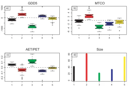
3.1 Description of clusters 3.1.1 Cluster 1

The first cluster is found predominantly in eastern Europe, although some sites are found in the centre of the continent. The sites cover a large latitudinal gradient, but, with the exception of a few sites in Greece, are not found at very low or high latitudes. The 20

sites are characterised by reduced GDD5 and increased moisture availability, and a mix of increased and decreased winter temperatures. The position of sites in this cluster suggests that it represents a zone of transition between the following two groups.

(10)

CPD

Full Screen / Esc

3.1.2 Cluster 2

This cluster is characterised by marked increases in GDD5 and coldest month temper-atures, and dryer conditions. The distribution is quite widespread, but is concentrated in the central and eastern regions, notably in the north-east. Such conditions are also found in a minority of Mediterranean sites.

5

3.1.3 Cluster 3

The third cluster has a restricted spatial distribution in which two sub-regions may be distinguished, one in the east and southeast and a second in the western part of the continent. This cluster shows, in contrast to cluster 2, decreased temperatures in both winter and summer, and increased moisture.

10

3.1.4 Cluster 4

With the exception of a few sites around the Black Sea and in Turkey, this cluster has a well-constrained distribution in sites close to the coast in the west of Europe. The sites are characterised by dryer conditions, together with increased GDD5 and decreased MTCO, suggesting a possible increase in seasonality.

15

3.1.5 Cluster 5

The final cluster has the most general geographic distribution of all groups, and is found across the continent. The cluster is comprised of sites that show little climatic change from today, with a slight cooling in winter.

3.2 Simulated clusters 20

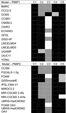
The main results of the comparison exercise for the models are summarised in Tables 2 and 3. Whilst most simulations appear to show a good agreement with the proxy data,

(11)

CPD

Full Screen / Esc

with between 3 and 5 of the clusters obtained, the majority of models are dominated by the first and fifth clusters. These two clusters show the smallest amount of change from the modern climate, and this result highlights the fact that the models simulate a smaller range of climate changes than those seen in the data. The standard deviation ratios obtained show that this difference in range may be as great as one fifth of the proxy data 5

range. As we wish to establish if a model is able to simulate the same direction and magnitude of change seen in the data, we have used these ratios to artificially inflate the model anomalies, and reassigned the model grid-points to clusters in a second comparison test. The distribution of clusters obtained is shown in Fig. 4 for both the PMIP1 and PMIP2 models. These results show that all models are able to simulate 10

the direction of change of four of the five clusters, and 9 PMIP1 models and 7 PMIP2 models are able to simulate the direction of change of all five clusters.

3.3 Variance and distances

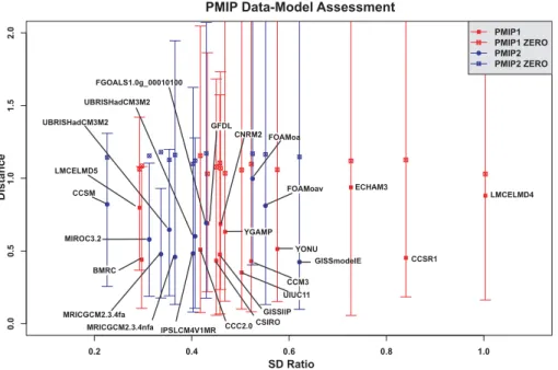
In order to compare between the different simulations, we have plotted each model as a function of the distances obtained between its simulated climate and the proxy clusters, 15

and the standard deviation ratio described above (Fig. 5). On this figure, a perfect fit between the model and data would have a distance of 0 and a standard deviation ratio of 1. The open symbols show the median distance obtained with the simulated modern climate. The figure shows that the median distance for the mid-Holocene simulation is lower than the modern simulation for all models and the majority of models are grouped 20

together, with a median distance of between 0.4 and 0.7 and a standard deviation ratio of between 0.3 and 0.5.

(12)

CPD

Full Screen / Esc

4 Discussion

4.1 Choice of proxy data

One important change in the current study from the previous mid-Holocene data-model comparison is the use of a new proxy dataset. The studies by Masson et al. (1998), Guiot et al. (1999), and Bonfils et al. (2004) all used the set of climate reconstructions of 5

produced by Cheddadi et al. (1997). As there are a number of differences between this reconstruction, and the estimations of Davis et al. (2003) used in the current study, it is worth briefly describing them and discussing the implications for comparative studies.

The radiocarbon dates used to attribute the pollen samples to the mid-Holocene were uncalibrated in Cheddadi et al. (1997) and calibrated in Davis et al. (2003). There will 10

therefore have been a difference in the fossil samples chosen to represent 6000 years BP. As no rapid or marked changes in mean climate or vegetation have been reported for this period, it is unlikely that this will have had a large effect on the reconstructed climate values. Both studies used a modern analogue technique to reconstruct climate, but with different constraining factors. The use of lake-levels as a constraint in the 15

Cheddadi et al study in particular appears to have reduced the amount of noise in the reconstructions. In their paper, Davis et al. (2003) compared their mid-Holocene results with those of Cheddadi et al, and noted that both studies showed a similar spatial structure with a generally warmer north and generally cooler south. This suggests that the directions of climate change that are used to test the models have not changed, 20

but the magnitude of those changes may be amplified in the Davis et al dataset. We have chosen to keep the dataset as it is attributed to the correct time period, but the interpretation of the standard deviation ratios presented above, must be made with care.

It should be also noted that the the anomaly maps of the reconstructed climatic vari-25

ables used are quite noisy: any two neighbouring sites may have neither the same magnitude nor even the same direction of change. This results in noisy maps and only the smoothed patterns have a climatic sense. The comparison with model maps

(13)

CPD

Full Screen / Esc

will therefore tend to underestimate the model fit to the data. This problem could be removed by using interpolated data maps, but this would artificially reduce the quantifi-cation of the errors. We consider it better to work on the original reconstructed data-set. 4.2 Comparison data-model

The clusters obtained for each model are summarised in Table 3 and Fig. 4. These 5

results show that whilst the same patterns of change are reproduced in nearly all the models, the spatial distribution of these changes varies widely. Three of the identified patterns of climate change (clusters 1, 4 and 5) are consistently reproduced. Cluster four was not seen in PMIP1 model CCM3, and the fifth cluster was absent from three PMIP2 models (FOAM, IPSL and MRI-CGCM2.3.4nfa). These clusters are all charac-10

terised by less extreme climate changes than the two other clusters (2 and 3), and it is unsurprising that they are frequently found in the models. However, these clusters do exhibit different trends of change: cluster 1 is slightly cooler and wetter and clus-ter 4 is dryer with increased GDD5. The models are therefore able to simulate complex patterns of change within a relatively restricted geographical area.

15

The second cluster is found in over the half the GCMs tested here, and in all models when an artificially expanded range of climate changes is considered, indicating that this pattern of change is always simulated, but changes are smaller than in the proxy reconstructions. The climate of this group is dryer and warmer than present, with increases in both winter temperature and GDD5. The increase in GDD5 follows the 20

increased summer insolation, a dominant forcing factor in the simulations (Joussaume et al., 1999). However, the increase in winter temperatures is more surprising, as winter insolation was lower during the mid-Holocene that today (Berger, 1978). Bonfils (2001) suggests that heating from humidity advection would have dominated the relatively weak decrease in insolation at high latitudes. The final group of changes (cluster 3) 25

was found in only one model (CCM3) in the first comparison test. The results of the second test, with inflated climate changes, show that this pattern of change is present in over half the models, but not the magnitude of change. Further, with the exception

(14)

CPD

Full Screen / Esc

of the FOAM GCM, it is consistently present in the PMIP2 simulations. This cluster represents the cooler and wetter climate of southern Europe during the mid-Holocene. Previous data-model comparison studies have shown that this climate pattern is rarely simulated for the mid-Holocene over Europe (Masson et al., 1998; Bonfils et al., 2004), as the increased summer insolation forces an increase in GDD5 (Masson et al., 1998). 5

A decrease in growing season length and intensity may, however, be controlled by a reduction in winter temperatures and increased summer evapotranspiration (Bonfils, 2001). The results of the tests presented here suggest that, as with the second cluster, the models are able to simulate this pattern of climate changes, if not the magnitude of the observed changes.

10

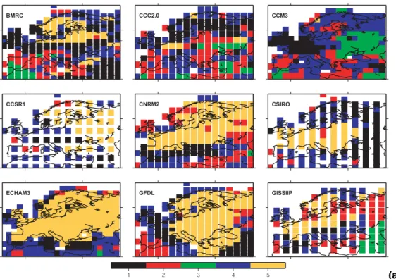
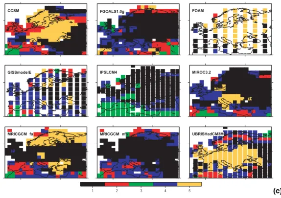
A visual comparison of the spatial distribution of the proxy clusters and the simu-lated clusters shows marked differences between the data and models and between the different models. Whilst a rigorous comparison is difficult, as the clusters of proxy sites are rarely well defined spatially, some generalisations may be made. A num-ber of models show the first cluster in the same location as the observed group 15

(BMRC, CCC2.0, CSIRO, UGAMP, UIUC11, FGOALS, GISSmodelE, IPSL-CM4-V1-MR, MIROC3.2, MRI-2.3.4fa, MRI-2.3.4nfa, FOAM-oav and UBRIS-oav). There is a good overlap between the distribution of second cluster in the data and several models (CCC2.0, CCM3, GISS-IIP, UGAMP, FGOALS, UBRIS-oa and UBRIS-oav), however, the cluster is rarely simulated as far north as it occurs in the data. The third cluster 20

is found in the south in some simulations (BMRC, CCM3, UGAMP, CCSM, IPSL-CM4-V1-MR, GISS-IIP, MIROC3.2, MRI2.3.4fa and MRI2.3.4nfa), but it is generally found further to the west than in the data. The coastal, northwestern location of cluster 4 is found in the majority of models. However, the simulated distribution is frequently more wide-spread than in the data. Finally, the wide-spread distribution of the fifth 25

cluster, representing a pattern of little climate change is also shown in the output from CNRM, CSIRO, ECHAM3, GFDL, GISS-IIP, LMCELMD4, LMCELMD5, YONU, CCSM, FOAM-oa, FOAM-oav, UBRIS-HadCM3M2-oa and UBRIS-HadCM3M2-oav).

(15)

CPD

Full Screen / Esc

4.3 Comparison model-model

In order to compare the simulations between the different models, we have plotted the range of Hagaman distances obtained against the ratio of anomaly standard deviations (Fig. 5). This shows that the majority of models have similar results and are grouped together, with a median distance of between 0.4 and 0.7 and a standard deviation ratio 5

of between 0.3 and 0.5. No obvious distinction can be made between the PMIP1 and PMIP2 models, suggesting that despite the increase in model complexity, there is no clear change in simulation results. This is perhaps a little surprising, as the PMIP2 models show a better ability to reproduce the problematic cool and wet cluster 3, how-ever models that best reproduce this cluster (e.g. IPSL-CM4-V1-MR and MIROC3.2) 10

have less success in reproducing the warm and dry pattern (cluster 2). An exception to this is the PMIP2 model GISSmodelE, which has a gradient of GDD5 anomalies over Europe that are very similar to those observed in the data, and thus reproduces the cooler south and warmer north. Of the models that fall outside of this group, one (CCSM) has a low ratio of standard anomalies and a relatively poor fit. The changes 15

simulated are relatively small, when compared to the other models, and the low fit may result in part from a reduced interannual variability. Three PMIP1 models are distinguished by high ratios of anomalies standard deviations (ECHAM3, CCSR1 and LMCELMD4). These models show a much larger range of changes, and notably, have much higher interannual variability.

20

The range of Hagaman distances obtained increases with the standard deviation ratio, as the possible difference between the simulated and observed values also in-creases. It is worth noting, however, that for two models (GISSmodelE and CCSR1), the median distance remains low, suggesting that the majority of simulated values of these models fit well to the data. In both these cases, the simulations produce geo-25

graphical gradients of anomalies that match well to the observed changes in GDD5 (GISSmodelE and MTCO (CCSR1).

Simulations were available from a flux-adjusted and non-flux-adjusted version of

(16)

CPD

Full Screen / Esc

one PMIP2 model, the coupled OA GCM from the Japanese Meteorological Re-search Institute (respectively MRI-CGCM2.3.4fa and MRI-CGCM2.3.4nfa). Both ver-sions of the model have a similar median Hagaman distance, suggesting the removal of flux-adjustment does not affect the general ability of this model to simulate the mid-Holocene climate of Europe. The non-flux-adjusted version does have a much larger 5

range of Hagaman distances, due mainly to a greater winter cooling in the north of Europe in this version of the model.

Two models were available from the PMIP2 project as coupled OA and coupled OAV versions (FOAM, UBRIS-HadCM3M2). In both cases, the inclusion of a coupled vege-tation model improves the output by increasing the range of anomalies simulated, thus 10

giving an output closer to the data values. The median Hagaman distance is improved for the FOAM model, although not for UBRIS-HadCM3M2. There is, however, no obvi-ous difference between the coupled OAV simulations and the main group of simulations on Fig. 5.

Finally, the test against zero anomalies (ZERO, Fig. 5) shows a higher median Haga-15

man distance than for the mid-Holocene simulation for all models. This indicates that in all cases, the simulated change under the mid-Holocene forcing follows the same direction of change as the data, and represents an improvement over the modern cli-matology.

5 Conclusions

20

We have used climate reconstructions from a dataset of fossil pollen sites to test to ability of a group of climate models of varying complexity to simulate the changes of the mid-Holocene climate over Europe. Using three climatic parameters, five patterns of climatic changes were identified in the data, ranging from cooler and wetter than present to warmer and dryer. A fuzzy logic approach was used to assign the model 25

simulations to these clusters, allowing the identification of the patterns that are sim-ulated by each model, and the geographic distribution of these patterns. Two tests

(17)

CPD

Full Screen / Esc

were made, a first based directly on simulated values, to assess the magnitude of the changes shown in each model. In the second test, the simulated values were adjusted to the data, allowing a better identification of the trends of climate change.

The results show that, whilst the models are not able to simulate the magnitude of the climate changes reconstructed in the pollen, they perform well in capturing the 5

different patterns of change, with four of the five patterns reproduced in the majority of models. Little distinction is shown between the first generation of atmosphere-only models and the newer coupled atmosphere-ocean models. In contrast, comparisons between different runs of the same model, with either different levels of complexity (FOAM, UBRIS-HadCM3M2) or removal of flux-adjustment, show improvements in the 10

range of values reconstructed. Further, the new generation PMIP2 models reproduce more successfully the pattern of cooler and wetter climate change in southern Europe than the previous models.

Despite their low spatial resolution, the models are capable of reproducing the quite complicated directions of change observed in a relatively restricted geographical area. 15

There remains a problem with the size of the simulated changes which are lower than those observed, although this is, in part, related to noise in the proxy reconstructions. Further, the spatial pattern of the simulated changes is frequently different from the data. In the region considered, the climatic changes for the mid-Holocene are rela-tively slight. Further work should apply this method to larger regions for which data 20

are available, e.g. the northern Hemisphere or to areas where large-scale changes in the climate have been observed, e.g. the African monsoon (Joussaume et al., 1999; Braconnot et al., 2000; Bonfils et al., 2001).

Acknowledgements. We acknowledge the international modeling groups for providing their

data for analysis, the Laboratoire des Sciences du Climat et de l’Environnement (LSCE) 25

for collecting and archiving the model data, and we thank P. Braconnot for helpful discus-sion on the method and its application. The PMIP2/MOTIF Data Archive is supported by CEA, CNRS, the EU project MOTIF (EVK2-CT-2002-00153) and the Programme National d’Etude de la Dynamique du Climat (PNEDC). The analyses were performed using version

(18)

CPD

Full Screen / Esc

11-20-2005 of the database. More information is available onhttp://www-lsce.cea.fr/pmip/and http://www-lsce.cea.fr/motif/.

References

Bardossy, A. and Duckstein, L.: Fuzzy Rule-Based Modelling with Applications to Geophysical, Biological, and Engineering Systems, Boca Raton, Florida, CRC Press, 256, 1995.

5

Berger, A. L.: Long-term variations of daily insolation and Quaternary climatic changes, J. Atmos. Sci., 35, 2362–2367, 1978.

Bonan, G. B.: A land surface model (LSM version 1.0) for ecological, hydrological, and atmo-spheric studies: technical description and user’s guide, NCAR Tech, 150, 1996.

Bonfils, C.: Le moyen-Holoc ène: r ôle de la surface continentale sur la sensibilit é climatique 10

simul ´ee, Paris, Universit ´e Paris VI, 322, 2001.

Bonfils, C., de Noblet-Ducoudre, N., Braconnot, P., and Joussaume, S.: Hot desert albedo and climate change: Mid-Holocene monsoon in North Africa, J. Climate, 17, 3724–3737, 2001. Bonfils, C., de Noblet-Ducoudre, N., Guiot, J., and Bartlein, P.: Some mechanisms of

mid-Holocene climate change in Europe, inferred from comparing PMIP models to data, Clim. 15

Dyn., 23, 79–98, 2004.

Braconnot, P. and Frankignoul, C.: Testing model simulations of the thermocline depth vari-ability in the tropical Atlantic from 1982 through 1984, J. Phys. Oceanogr., 23, 626–647, 1993.

Braconnot, P., Joussaume, S., de Noblet, N., and Ramstein, G.: Mid-Holocene and Last Glacial 20

Maximum African monsoon changes as simulated within the Paleoclimate Modeling Inter-comparison Project, Global and Planetary Change, 26, 51–66, 2000.

Brewer, S., Alleaume, S., Guiot, J., and Nicault, A.: Historical droughts in Mediterranean re-gions during the last 500 years: a data/model approach, Clim. Past Discuss., 2, 771–800, 2006,

25

http://www.clim-past-discuss.net/2/771/2006/.

Cheddadi, R., Yu, G., Guiot, J., Harrison, S. P., and Prentice, I. C.: The climate of Europe 6000 years ago, Clim. Dyn., 13, 1–9, 1997.

Collins, W. D., Bitz, C. M., Blackmon, M. L., Bonan, G. B., Bretherton, C. S., Carton, J. A., Chang, S., Doney, C., Hack, J. J., Henderson, T. B., Kiehl, J. T., Large, W. G., McKenna, 30

(19)

CPD

Full Screen / Esc

D. S., Santer, B. D., and Smith, R. D.: The Community Climate System Model (CCSM3), J. Climate, 19, 2122–2143, 2006.

Davis, B. A. S., Brewer, S., Stevenson, A. C., Guiot, J., and Data Contributors: The temperature of Europe during the Holocene reconstructed from pollen data, Quat. Sci. Rev., 22, 1701– 1716, 2003.

5

Deque, M., Dreveton, C., Braun, A., and Cariolle, D.: The ARPEGE/IFS atmosphere model: A contribution to the French community climate modelling, Clim. Dyn., 10, 249–266, 1994. Deutsches Klimarechenzentrum (DKRZ) Modellbetreuungsgruppe: The ECHAM3 atmospheric

general circulation model, DKRZ Tech. Report, 184pp, 1992.

Gordon, C., Cooper, C., Senior, C. A., Banks, H., Gregory, J. M., Johns, T. C., Mitchell, J. 10

F. B., and Wood, R. A.: The simulation of SST, sea ice extents and ocean heat transports in a version of the Hadley Centre coupled model without flux adjustments, Clim. Dyn., 16, 147–168, 2000.

Gordon, C. T. and Stern, W. F.: A description of the GFDL global spectral model, Mon. Wea. Rev., 110, 625–644, 1982.

15

Gordon, H. B. and O’Farrell, S. P.: Transient Climate Change in the CSIRO Coupled Model with Dynamic Sea Ice, Mon. Wea. Rev., 125, 875–907, 1997.

Guiot, J., Boreux, J. J., Braconnot, P., Torre, F., and PMIP participating groups: Data-model comparisons using fuzzy logic in palaeoclimatology, Clim. Dyn., 15, 569–581, 1999.

Hall, N. M. J. and Valdes, P. J.: A GCM simulation of the climate 6000 years ago, J. Climate, 20

10, 3–17, 1997.

Hansen, J. E., Sato, M., Ruedy, R., Lacis, A. A., Asamoah, K., Beckford, K., Borenstein, S., Brown, E., Cairns, B., Carlson, B., Curran, B., de Castro, S., Druyan, L., Etwarrow, P., Ferede, T., Fox, M., Gaffen, D., Glascoe, J., Gordon, H. B., Hollandsworth, S., Jiang, X., Johnson, C., Lawrence, N., Lean, J., Lerner, J., Lo, K. K., Logan, J., Luckett, A., McCormick, M. P., 25

McPeters, R., Miller, R. L., Minnis, P., Ramberran, I., Russell, G., Russel, P., Stone, P. H., Tegen, I., Thomas, S., Thomason, L., Thompson, A., Wilder, J., Willson, R., and Zawodny, J.: Forcings and chaos in interannual to decadal climate change., J. Geophys. Res., 102, 25 679–25 720, 1997.

Harrison, S. P., Jolly, D., Laarif, F., Abe-Ouchi, A., Herterich, K., Hewitt, C., Joussaume, S., 30

Kutzbach, J. E., Mitchell, J., Noblet, N. D., and Valdes, P.: Intercomparison of simulated global vegetation distributions in response to 6kyr BP orbital forcing, J. Climate, 11, 2721– 2742, 1998.

(20)

CPD

Full Screen / Esc

Hartigan, J. A. and Wong, M. A.: A K-means clustering algorithm, Applied Statistics, 28, 100– 108, 1979.

Harzallah, A. and Sadourny, R.: Internal versus SST-forced atmospheric variability as simulated by an atmospheric general circulation model, J. Climate, 8, 474–495, 1995.

Joussaume, S. and Taylor, K.: Status of the Paleoclimate Modeling Intercomparison Project 5

(PMIP), 92, 425–430, 1995.

Joussaume, S., Taylor, K. E., Braconnot, P., Mitchell, J. F. B., Kutzbach, J. E., Harrison, S. P., Prentice, I. C., Broccoli, A. J., Abe-Ouchi, A., Bartlein, P. J., Bonfils, C., Dong, B., Guiot, J., Herterich, K., Hewitt, C. D., Jolly, D., Kim, J. W., Kislov, A., Kitoh, A., Loutre, M. F., Masson, V., McAvaney, B., McFarlane, N., de Noblet, N., Peltier, W. R., Peterschmitt, J. Y., 10

Pollard, D., Rind, D., Royer, J. F., Schlesinger, M. E., Syktus, J., Thompson, S., Valdes, P., Vettoretti, G., Webb, R. S., and Wyputta, U.: Monsoon changes for 6000 years ago: results of 18 simulations from the Paleoclimate Modeliing Intercomparison Project (PMIP), Geophys. Res. Lett., 26, 859–862, 1999.

K-1 model developers: K-1 coupled model (MIROC) description, 34, 2004. 15

Kim, J.-H. and Schneider, R. R.: GHOST global database for alkenone-derived Holocene sea-surface temperature records.,http://www.pangaea.de/Projects/GHOST/, 2004.

Liao, X., Street-Perrott, F., and Mitchell, J.: GCM experiments with different cloud parame-terization: comparisons with palaeoclimatic reconstructions for 6000 years BP, Data and Modelling, 1, 99–123, 1994.

20

Marti, O., Braconnot, P., Bellier, J., Benshila, R., Bony, S., Brockmann, P., Cadulle, P., Caubel, A., Denvil, S., Dufresne, J. L., Fairhead, L., Filiberti, M.-A., Fichefert, T., Friedlingstein, P., Grandpeix, J.-Y., Hourdin, F., Krinner, G., L ´evy, C., Musat, I., Talandier, C., and the IPSL Global Climate Modeling Group: The new IPSL climate system model: IPSL-CM4, 86,http: //dods.ipsl.jussieu.fr/omamce/IPSLCM4/DocIPSLCM4/FILES/DocIPSLCM4.pdf, 2005. 25

Masson, V., Cheddadi, R., Braconnot, P., Joussaume, S., Texier, D., and Participants, P.: Mid-Holocene climate in Europe: what can we infer from PMIP model-data comparisons?, Clim. Dyn., 15, 163–182, 1998.

McAvaney, B. J. and Colman, R. A.: The BMRC Model: AMIP configuration, BMRC Research Report, 43, 1993.

30

McFarlene, N. A., Boer, G. J., Blanchet, J.-P., and Lazare, M.: The Canadian Climate Cen-tre Second-Generation General Circulation Model and its equilibrium climate, J. Climate, 5, 1013–1044, 1992.

(21)

CPD

Full Screen / Esc

Numagati, A., Takahashi, M., Nakajima, T., and Sumi, A.: Development of an atmospheric general circulation model, in: Climate System Dynamics and Modelling, Tokyo, edited by: Matsuno, T., University of Tokyo, 1–27, 1995.

Prentice, I. C., Harrison, S., Jolly, D., and Guiot, J.: The climate and biomes of Europe at 6000 yr BP: comparison of model simulations and pollen-based reconstructions, Quat. Sci. 5

Rev., 17, 659–668, 1998.

Prentice, I. C., Jolly, D., and Participants, B.: Mid-Holocene and glacial-maximum vegetation geography of the northern continents and Africa, J. Biogeography, 27, 507–519, 2000. Sadourny, R. and Laval, K.: January and July performance of the LMD general circulation

model, in: New Perspectives in Climate Modelling, edited by: Berger, A. L. and Nicolis, C., 10

Developments in Atmospheric Science, 16, Elsevier, 173–198, 1984.

Schlesinger, M. E., Andronova, N. G., Entwhistle, B., Ghanem, A., Ramankutty, N., Wang, W., and Yang, F.: Modeling and Simulation of Climate and Climate Change, In Past and present variability of the solar-terrestrial system: Measurements, data analysis and theoretical mod-els, in: Proceedings of the International School of Physics “Enrico Fermi”, Course CXXXIII, 15

Varrena, Italy, edited by: Cini Castagnoli, G. and Provenzale, A., OS Press, Amsterdam, 389–429, 1997.

Schmidt, G. A., Ruedy, R., Hansen, J. E., Aleinov, I., Bell, N., Bauer, M., Bauer, S., Cairns, B., Canuto, V., Cheng, Y., Del Denio, A., Faluvegi, G., Friend, A. D., Hall, T. M., Hu, Y., Kelly, M., Kiang, N. Y., Koch, D., Lacis, A. A., Lerner, J., Lo, K. K., Miller, R. L., Nazarenko, 20

L., Oinas, V., Perlwitz, J., Perlwitz, J., Rind, D., Romanou, A., Russell, G. L., Sato, M., Shindell, D. T., Stone, P. H., Sun, S., Tausnev, N., Thresher, D., and Yao, M.-S.: Present day atmospheric simulations using GISS ModelE: Comparison to in-situ, satellite and reanalysis data, J. Climate, 19, 153–192, 2006.

Texier, D., Noblet, N. d., Harrison, S., Haxeltine, A., Jolly, D., Laarif, F., Prentice, I. C., and 25

Tarasov, P.: Quantifying the role of biosphere-atmosphere feedbacks in climate change: coupled model simulations for 6000 years BP and comparison with paleodata for northern Eurasia and northern Africa, Clim. Dyn., 13, 865–882, 1997.

Tokioka, T., Yamazaki, K., Yagai, I., and Kitoh, A.: A description of the Meteorological Research Institute atmospheric general circulation model (MRI GCM-I), MRI Tech. Report No. 13, 249, 30

1984.

Wright Jr, H. E., Kutzbach, J. E., Webb III, T., Ruddiman, W. F., Street-Perrott, F., and Bartlein, P. J.: Global Climates since the Last Glacial Maximum, 544, 1993.

(22)

CPD

Full Screen / Esc

Yu, Y., Zhang, X., and Guo, Y.: Global coupled ocean-atmosphere general circulation models in LASG/IAP, Adv. Atmos. Sci., 21, 444–455, 2004.

Yukimoto, S., Noda, A., Kitoh, A., Sugi, M., Kitamura, Y., Hosaka, M., Shibata, K., Maeda, S., and Uchiyama, T.: The New Meteorological Research Institute Coupled GCM (MRI-CGCM2): Model Climate and Variability, Papers in Meteorology and Geophysics, 51, 47–88, 2001. 5

(23)

CPD

Full Screen / Esc

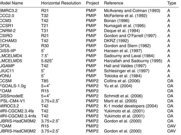
Table 1. GCMs included in the comparison study. Note that this does not include all models

available in the PMIP projects, only those for which all necessary information was available. For coupled models, the resolution is given for the atmospheric component. For details of the FOAM OA and OAV model, please refer to the PMIP2/MOTIF website:http://www-lsce.cea.fr/ motif/.

Model Name Horizontal Resolution Project Reference Type

BMRC3.2 R21 PMIP McAvaney and Colman (1993) A

CCC2.0 T32 PMIP McFarlene et al. (1992) A

CCM3 T42 PMIP Bonan (1996) A

CCSR1 T21 PMIP Numagati et al. (1995) A

CNRM-2 T31 PMIP Deque et al. (1994) A

CSIRO R21 PMIP Gordon and O’Farrell (1997) A

ECHAM3 T42 PMIP DKRZ (1992) A

GFDL R30 PMIP Gordon and Stern (1982) A

GISS-IIP 5◦ _PMIP _{Hansen et al. (1997)} _A

LMCELMD4 7.5◦ _PMIP _{Sadourny and Laval (1984)} _A

LMCELMD5 5.625◦ _PMIP _{Harzallah and Sadourny (1995)} _A

UGAMP T42 PMIP Hall and Valdes (1997) A

UIUC11 5◦ _PMIP _{Schlesinger et al. (1997)} _A

YONU 5◦ _PMIP _{Tokioka et al. (1984)} _A

CCSM T85 PMIP2 Collins et al. (2006) OA

FGOALS-1.0g 5×4◦ PMIP2 Yu et al. (2004) OA

FOAM R15 PMIP2 OA

GISSmodelE 5×4◦ PMIP2 Schmidt et al. (2006) OA

IPSL-CM4-V1 3.75×2.5◦ _PMIP2 _{Marti et al. (2005)} _OA

MIROC3.2 T42 PMIP2 K-1 model developers (2004) OA

MRI-CGCM2.3.4fa T42 PMIP2 Yukimoto et al. (2001) OA

MRI-CGCM2.3.4nfa T42 PMIP2 Yukimoto et al. (2001) OA

UBRIS-HadCM3M2 3.75×2.5◦ _PMIP2 _{Gordon et al. (2000)} _OA

FOAM R15 PMIP2 OAV

UBRIS-HadCM3M2 3.75×2.5◦ _PMIP2 _{Gordon et al. (2000)} _OAV

(24)

CPD

Full Screen / Esc

Table 2. Standard deviation of cluster centroids. The second row gives the standard deviation

of the clusters belonging to the single dominant cluster solution. GDD5 MTCO AET/PET

All runs 101.46 0.39 0.021

Selected solution 19.71 0.16 0.003

(25)

CPD

Full Screen / Esc

Table 3. Simulated clusters by model. Black squares indicate that the cluster is simulated in

both the first comparison based on simulated anomalies, and the second comparison based on adjusted simulated anomalies. Gray squares represent clusters found only in the second comparison. White squares represent cluster that were not found in either comparison.

Model – PMIP1 C1 C2 C3 C4 C5 BMRC CCC2.0 CCM3 CCSR1 CNRM-2 CSIRO ECHAM3 GFDL GISS-IIP LMCELMD4 LMCELMD5 UGAMP UIUC11 YONU Model – PMIP2 C1 C2 C3 C4 C5 CCSM FGOALS-1.0g FOAM GISSmodelE IPSL-CM4-V1 MIROC3.2 MRI-CGCM2.3.4fa MRI-CGCM2.3.4nfa UBRIS-HadCM3M2 FOAM OAV UBRIS-HadCM3M2 OAV 1178

(26)

CPD

Full Screen / Esc

Printer-friendly Version Interactive Discussion 1500 1000 500 0 500 1000 1500 a) MTCO 0 250 500 750 1000 1250 1500 b) MTCO S D 6 4 2 0 2 4 6 c) G DD5 0 2 4 6 8 d) G DD5 S D 0. 2 0. 1 0.0 0.1 0.2 e) AET/PET 0.00 0.05 0.10 0.15 0.20 f) AET/PET S D

Fig. 1. Maps showing the distribution of mid-Holocene pollen sites used in the comparison,

together with the reconstructed anomalies and the standard deviation of the reconstruction:

(a) Mean temperature of the coldest month (MTCO); (b) MTCO standard deviation; (c)

Grow-ing Degree Days Over 5◦_{C (GDD5); (d) GDD5 standard deviation; (e) Actual}

evapotranspira-tion/potential evapotranspiration (AET/PET); (f) AET/PET standard deviation. 1179

(27)

CPD

Full Screen / Esc

Printer-friendly Version Interactive Discussion 1 2 3 4 5 a) All clusters 1 2 3 4 5 b) Cluster 1 1 2 3 4 5 c) Cluster 2 1 2 3 4 5 d) Cluster 3 1 2 3 4 5 e) Cluster 4 1 2 3 4 5 f) Cluster 5

Fig. 2. Maps showing the distribution of the 5 climatically defined clusters used in the

compar-ison.

(28)

CPD

Full Screen / Esc

Printer-friendly Version Interactive Discussion Size AET/PET GDD5 MTCO a) b) c) d) 1 2 3 4 5 1 2 3 4 5 1 2 3 4 5 1 2 3 4 5 0.0 0.1 0.2 -0.1 -0.2 ₀₄ 0 20 60 80 0 1000 -1000 0 -2 -4 -6 2 4 6

Fig. 3. Climatic characteristics of the 5 clusters, in terms of the three parameters used: (a) GDD5; (b) MTCO; (c) AET/PET; (d) cluster size.

(29)

CPD

Full Screen / Esc

Printer-friendly Version Interactive Discussion BMRC CCC2.0 CCM3 CCSR1 CNRM2 CSIRO ECHAM3 GFDL GISSIIP 1 2 3 4 5 (a)

Fig. 4. Geographic distribution of clusters obtained for each model. (a) and (b) PMIP1 models; (c) PMIP2 OA coupled models; (d) PMIP2 OAV coupled models.

(30)

CPD

Full Screen / Esc

Printer-friendly Version Interactive Discussion b)

LMCELMD4 LMCELMD5 UGAMP

UIUC11 YONU 1 2 3 4 5 c) (b) Fig. 4. Continued. 1183

(31)

CPD

Full Screen / Esc

CCSM FGOALS1.0g FOAM

GISSmodelE IPSLCM4 MIROC3.2

MRICGCM fa MRICGCM nfa UBRISHadCM3M2

1 2 3 4 5 (c)

Fig. 4. Continued.

(32)

CPD

Full Screen / Esc

Printer-friendly Version Interactive Discussion FOAM O AV UBRISHadCM3M2 O AV 1 2 3 4 5 _(d) Fig. 4. Continued. 1185

(33)

CPD

Full Screen / Esc

Printer-friendly Version Interactive Discussion 0.2 0.4 0.6 0.8 1.0 0 .0 0 .5 1 .0 1 .5 2 .0

PMIP Data-Model Assessment

SD Ratio D is ta n c e PMIP1 PMIP1 ZERO PMIP2 PMIP2 ZERO FGOALS1.0g_00010100 UBRISHadCM3M2 UBRISHadCM3M2 LMCELMD5 CCSM MIROC3.2 BMRC CCC2.0 GFDL GISSIIP CSIRO CNRM2 YGAMP UIUC11 CCM3 GISSmodelE YONU FOAMoa FOAMoav ECHAM3 CCSR1 LMCELMD4 MRICGCM2.3.4fa MRICGCM2.3.4nfa IPSLCM4V1MR

Fig. 5. Results of final comparison. Each model is represented by a bar describing the range

of Hagaman distances obtained. The limits of the bar are the 5th and 95th percentile and the median distance is shown by a closed symbol. The open symbols are the results of the comparison using zero anomalies, i.e. the modern simulated climate. The position of the bars on the x-axis represents the ratio between the range of simulated and observed values. On this figure, a model with a perfect fit to the data would have a distance of zero and a ratio of values of 1.