HAL Id: hal-01411370
https://hal.univ-grenoble-alpes.fr/hal-01411370
Submitted on 30 Oct 2020
HAL is a multi-disciplinary open access
archive for the deposit and dissemination of
sci-entific research documents, whether they are
pub-lished or not. The documents may come from
teaching and research institutions in France or
abroad, or from public or private research centers.
L’archive ouverte pluridisciplinaire HAL, est
destinée au dépôt et à la diffusion de documents
scientifiques de niveau recherche, publiés ou non,
émanant des établissements d’enseignement et de
recherche français ou étrangers, des laboratoires
publics ou privés.
perfluorocarbons CF4, C2F6 and C3F8 since 1800
inferred from ice core, firn, air archive and in situ
measurements
Cathy M. Trudinger, Paul J. Fraser, David M. Etheridge, William T. Sturges,
Martin K. Vollmer, Matt Rigby, Patricia Martinerie, Jens Mühle, David R.
Worton, Paul B. Krummel, et al.
To cite this version:
Cathy M. Trudinger, Paul J. Fraser, David M. Etheridge, William T. Sturges, Martin K. Vollmer,
et al.. Atmospheric abundance and global emissions of perfluorocarbons CF4, C2F6 and C3F8 since
1800 inferred from ice core, firn, air archive and in situ measurements. Atmospheric Chemistry and
Physics, European Geosciences Union, 2016, 16 (18), pp.11733 - 11754. �10.5194/acp-16-11733-2016�.
�hal-01411370�
www.atmos-chem-phys.net/16/11733/2016/ doi:10.5194/acp-16-11733-2016
© Author(s) 2016. CC Attribution 3.0 License.
Atmospheric abundance and global emissions of perfluorocarbons
CF
4
, C
2
F
6
and C
3
F
8
since 1800 inferred from ice core, firn, air
archive and in situ measurements
Cathy M. Trudinger1, Paul J. Fraser1, David M. Etheridge1, William T. Sturges2, Martin K. Vollmer3, Matt Rigby4, Patricia Martinerie5, Jens Mühle6, David R. Worton7, Paul B. Krummel1, L. Paul Steele1, Benjamin R. Miller8, Johannes Laube2, Francis S. Mani9, Peter J. Rayner10, Christina M. Harth6, Emmanuel Witrant11,
Thomas Blunier12, Jakob Schwander13, Simon O’Doherty4, and Mark Battle14 1CSIRO Oceans and Atmosphere, Aspendale, Victoria, Australia
2Centre for Ocean and Atmospheric Sciences, School of Environmental Sciences, University of East Anglia, Norwich, NR4 7TJ, UK
3Laboratory for Air Pollution and Environmental Technology, Empa, Swiss Federal Laboratories for Materials Science and Technology, Dübendorf, Switzerland
4School of Chemistry, University of Bristol, Bristol, UK
5UJF-Grenoble 1/CNRS, Laboratoire de Glaciologie et Géophysique de l’Environnement, 38041 Grenoble, France 6Scripps Institution of Oceanography, University of California at San Diego, La Jolla, California, USA
7National Physical Laboratory, Hampton Road, Teddington, Middlesex, TW11 0LW, UK
8Cooperative Institute for Research in Environmental Sciences, University of Colorado, Boulder, USA 9School of Biological and Chemical Sciences, University of the South Pacific, Suva, Fiji
10School of Earth Sciences, University of Melbourne, Australia
11UJF-Grenoble 1/CNRS, Grenoble Image Parole Signal Automatique, Grenoble, France
12Center for Ice and Climate, Niels Bohr Institute, University of Copenhagen, Copenhagen, Denmark 13Climate and Environmental Physics, Physics Institute and Oeschger Centre for Climate Change Research, University of Bern, Bern, Switzerland
14Department of Physics and Astronomy, Bowdoin College, Maine, USA
Correspondence to:Cathy M. Trudinger (cathy.trudinger@csiro.au)
Received: 18 May 2016 – Published in Atmos. Chem. Phys. Discuss.: 6 June 2016 Revised: 25 August 2016 – Accepted: 5 September 2016 – Published: 21 September 2016
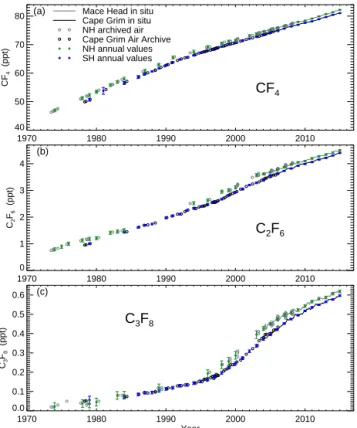
Abstract. Perfluorocarbons (PFCs) are very potent and long-lived greenhouse gases in the atmosphere, released pre-dominantly during aluminium production and semiconductor manufacture. They have been targeted for emission controls under the United Nations Framework Convention on Climate Change. Here we present the first continuous records of the atmospheric abundance of CF4 (PFC-14), C2F6 (PFC-116) and C3F8(PFC-218) from 1800 to 2014. The records are de-rived from high-precision measurements of PFCs in air ex-tracted from polar firn or ice at six sites (DE08, DE08-2, DSSW20K, EDML, NEEM and South Pole) and air archive tanks and atmospheric air sampled from both hemispheres. We take account of the age characteristics of the firn and
ice core air samples and demonstrate excellent consistency between the ice core, firn and atmospheric measurements. We present an inversion for global emissions from 1900 to 2014. We also formulate the inversion to directly infer emis-sion factors for PFC emisemis-sions due to aluminium production prior to the 1980s. We show that 19th century atmospheric levels, before significant anthropogenic influence, were sta-ble at 34.1 ± 0.3 ppt for CF4 and below detection limits of 0.002 and 0.01 ppt for C2F6and C3F8, respectively. We find a significant peak in CF4and C2F6emissions around 1940, most likely due to the high demand for aluminium during World War II, for example for construction of aircraft, but these emissions were nevertheless much lower than in recent
years. The PFC emission factors for aluminium production in the early 20th century were significantly higher than today but have decreased since then due to improvements and bet-ter control of the smelting process. Mitigation efforts have led to decreases in emissions from peaks in 1980 (CF4) or early-to-mid-2000s (C2F6 and C3F8) despite the continued increase in global aluminium production; however, these de-creases in emissions appear to have recently halted. We see a temporary reduction of around 15 % in CF4emissions in 2009, presumably associated with the impact of the global financial crisis on aluminium and semiconductor production.
1 Introduction
Perfluorocarbons (PFCs) are very potent greenhouse gases
(about 7000–11 000 times more powerful than CO2 on a
weight-emitted basis over a 100-year timescale; Myhre et al., 2013). They are very long-lived in the atmosphere, making them of particular relevance for achieving climate stabili-sation. We will focus here on three PFCs, CF4, C2F6 and C3F8, but there are other PFCs in the atmosphere with lower abundance than CF4and C2F6(e.g. Oram et al., 2012; Laube et al., 2012).
CF4(carbon tetrafluoride, PFC-14) is the most abundant perfluorocarbon in the atmosphere (Mühle et al., 2010). It is released predominantly from aluminium production (due to so-called “anode effects”, when the feed of aluminum ox-ide to or within the electrolysis cell is restricted; Holiday and Henry, 1959; Tabereaux, 1994) and during semicon-ductor manufacture (Tsai et al., 2002; Khalil et al., 2003). There is a small natural source from rocks (fluorites and granites) released by tectonic activity and weathering (Har-nisch and Eisenhauer, 1998; Deeds et al., 2008, 2015; Mulder et al., 2013; Schmitt et al., 2013). Other very small indus-trial sources of CF4include release during production of SF6 and HCFC-22 (Institute for Environmental Protection and Research, 2013) and from UV photolysis of trifluoroacetyl fluoride, which is a degradation product of halocarbons such as HFC-134a, HCFC-124 and CFC-114a (Jubb et al., 2015). Another possible source of CF4 is from the rare earth in-dustry, particularly in China, specifically neodymium ox-ide electrolysis (Vogel and Friedrich, 2015). However, these other sources of emissions have been negligible to date com-pared to the CF4emissions due to aluminium production and semiconductor manufacture (Harnisch and Eisenhauer, 1998; Jubb et al., 2015; Wong et al., 2015).
C2F6 (perfluoroethane, PFC-116) is released predom-inantly during aluminium production and semiconductor manufacture (Tsai et al., 2002; Fraser et al., 2013). It is also used in the R-508 refrigerant blend, although emissions are believed to be small compared to the other sources (Kim et al., 2014). C3F8(perfluoropropane, PFC-218) is the least abundant of these three PFCs and is used as a refrigerant
as well as being released during semiconductor manufacture (EDGAR, 2010; Tsai et al., 2002). C3F8has been detected at low levels in emissions from aluminium smelters (Fraser et al., 2013; Li et al., 2012). The aluminium industry does not currently account for C3F8emissions (International Alu-minium Institute, 2014) or include them in the current IPCC guidelines for bottom up accounting of PFC emissions from aluminium production (IPCC, 2006), but due to the low lev-els compared to the other PFCs (Fraser et al., 2013; Li et al., 2012) C3F8 is likely to be difficult to detect with the mea-surement systems used by the aluminium industry. Natural sources of C2F6and C3F8have not been identified (Harnisch, 1999).
Sinks of these PFCs are dominated by unintentional thermal destruction during high-temperature combustion at ground level, giving atmospheric lifetimes for CF4, C2F6and C3F8 of about 50 000, 10 000 and 2600 years, respectively (Cicerone, 1979; Morris et al., 1995; Myhre et al., 2013). PFCs have been targeted by both the aluminium and semi-conductor industries for emission controls to reduce green-house gas emissions.
Atmospheric measurements of greenhouse gases are the only reliable way to verify estimates of global emissions to ensure that we can predict the effect of emissions on radia-tive forcing and to guide mitigation options. Mühle et al. (2010) gave a summary of previous measurements of CF4, C2F6and C3F8, then presented new high-precision measure-ments from 1973 to 2008 on air from (a) the Cape Grim Air Archive (Langenfelds et al., 1996), (b) a suite of tanks with old northern hemispheric air and (c) the Advanced Global Atmospheric Gases Experiment (AGAGE) in situ at-mospheric monitoring network. They presented estimates of global trends in PFC abundance and the corresponding sions from 1973 to 2008. They showed that global emis-sions peaked in 1980 (CF4) or early-to-mid-2000s (C2F6 and C3F8) before decreasing due to mitigation efforts by both the aluminium and semiconductor industries. The emis-sions estimates based on atmospheric measurements were significantly higher than previous estimates based on inven-tories. Kim et al. (2014) extended this work using mea-sured C2F6/CF4 emission ratios specific to the aluminium and semiconductor industries to partition global emissions to each industry. They suggested that underestimated emissions from the global semiconductor industry during 1990–2010 and China’s aluminium industry after 2002 accounted for the discrepancy between PFC emissions based on atmospheric measurements and inventories. Underestimated PFC sions may also be from previously unaccounted-for emis-sions from aluminium production due to undetected anode effects (Wong et al., 2015).
Air extracted from firn (the layer of unconsolidated snow overlying an ice sheet) or bubbles in polar ice provides a re-liable way to reconstruct atmospheric composition prior to direct atmospheric measurements. Mühle et al. (2010) es-timated the pre-industrial, natural background abundances
from firn air at the Megadunes site in Antarctica (air with a mean age of about AD 1910) and air from 11 samples of melted glacial ice at Pâkitsoq in Greenland (with ages be-tween 19 000 and 11 360 BP) to be 34.7 ± 0.2 ppt for CF4 (based on both Megadunes and Pâkitsoq) and 0.1 ± 0.02 ppt for C2F6(based on Megadunes alone). Worton et al. (2007) used firn measurements from the North Greenland ice core project site (NGRIP) and Berkner Island, Antarctica, to re-construct CF4 from the mid-1950s and C2F6 from 1940 to present. However, these previous records from firn and ice are not continuous through from pre-industrial to recent lev-els.
Here we present measurements of CF4, C2F6and C3F8in air extracted from four firn sites (DSSW20K, EDML, NEEM 2008 and South Pole 2001) and two ice cores (DE08 and DE08-2). We combine these with the air archive and in situ measurements from Mühle et al. (2010), extended to the end of 2014, and use an inversion calculation to estimate global emissions, with uncertainties, and show how these PFCs have varied in the atmosphere from pre-anthropogenic levels in the 19th century to 2014. We also reformulate our inversion to directly infer emission factors for PFC emissions due to aluminium production for the period up to 1980 when alu-minium production dominates PFC emissions.
2 Methods
2.1 Data – locations, measurement and calibration
scales
The firn and ice core measurements used in this work come from ice or firn air collected at the following sites:
– DE08 and DE08-2 are located 16 km east of the sum-mit of Law Dome (66.7◦S, 112.8◦E) in East Antarc-tica (Etheridge et al., 1996, 1998). They are 300 m apart and have nearly identical site characteristics, including very high snow accumulation rates (1100 kg m−2yr−1). Ice cores were drilled at DE08 and DE08-2 in 1987 and 1993, respectively.
– DSSW20K is 20 km west of the deep DSS (Dome Summit South) drill site near the summit of Law Dome in East Antarctica (Smith et al., 2000; Sturrock et al., 2002; Trudinger et al., 2002). DSSW20K has a short firn column and a moderate snow accumulation rate (150 kg m−2yr−1). Firn air was collected in Jan-uary 1998.
– EDML (EPICA Dronning Maud Land) is the EPICA
drill site near Kohnen Station (75.2◦S, 0.1◦E),
in Dronning Maud Land, Antarctica (Weiler, 2008; Mani, 2010). It has a low snow accumulation rate (65 kg m−2yr−1) and firn air was collected in Jan-uary 2006.
– NEEM 2008 firn air was extracted from a borehole near the NEEM (North Greenland Eemian Ice Drilling Project) deep ice core drilling site (77.5◦N, 51.1◦W) in northern Greenland (Buizert et al., 2012). NEEM has a moderate snow accumulation rate (199 kg m−2yr−1). We use air from the EU borehole collected in July 2008. – South Pole 2001, Antarctica (90◦S), has a deep firn and a low snow accumulation rate (74 kg m−2yr−1) (Butler et al., 2001; Aydin et al., 2004; Sowers et al., 2005). Here we measure only one sample from the South Pole, collected in 2001 from 120 m.
In addition to the firn and ice core measurements, we use archived and in situ measurements from Mühle et al. (2010), extended to the end of 2014 and focused on the high latitudes in each hemisphere.
Measurements were made using two different ment systems and primary calibration scales. The measure-ments in Mühle et al. (2010) were made on Medusa sys-tems (Miller et al., 2008) and reported on Scripps Institu-tion of Oceanography (SIO) primary calibraInstitu-tion scales (SIO-05 for CF4and SIO-07 for C2F6and C3F8). Measurements of firn air from DSSW20K, NEEM 2008 and South Pole 2001 were made at CSIRO (Aspendale) or Cape Grim on the Medusa system and are also reported on SIO calibra-tion scales. Air was extracted from DE08 and DE08-2 ice in ICELAB at CSIRO (Aspendale) using a “cheese grater” dry extraction system (Etheridge et al., 1988). Air from the DE08 and DE08-2 ice cores and the EDML firn was anal-ysed at the University of East Anglia (UEA) using high-sensitivity gas chromatograph/trisector mass spectrometer system (Waters/Micromass Autospec) (Worton et al., 2007; Sturges et al., 2001; Mani, 2010). Measurements made at UEA are reported on UEA calibration scales. We derive con-version factors between the two calibration scales in Ap-pendix A and report all measurements on the SIO-05 (CF4) and SIO-07 (C2F6and C3F8) primary calibration scales. Fur-ther measurement details are available in Appendix B. The firn, ice core and archive measurements are available in the Supplement. The in situ measurements are available on the CDIAC website (Prinn et al., 2016).
2.2 Firn model
To characterise the age of the air in the firn and ice sam-ples, we use a numerical model of the processes that occur in firn and ice (mainly diffusion of air in the firn layer, ad-vection of snow downwards as new snow falls at the surface and gradual trapping of the air into bubbles). These processes mean that air contained in firn or ice corresponds to atmo-spheric air over a range of times rather than a single age. We use the CSIRO firn model (Trudinger et al., 1997), up-dated by Trudinger et al. (2013), and the LGGE-GIPSA firn model (Witrant et al., 2012) to characterise the air age and
age spread. We use the two independent models as a way to incorporate firn model uncertainty.
The depth profile of diffusivity in the firn and other diffusivity-related parameters in the firn models need to be calibrated for each site that we model. To do this we tune the models to fit firn measurements of trace gases for which we know the past atmospheric history. Calibration of the CSIRO firn model for DE08 and DE08-2 (which are mod-elled as identical sites), as well as DSSW20K, NEEM 2008 and South Pole 2001, is described in Trudinger et al. (2013), and for EDML in Appendix C. Calibration of the LGGE-GIPSA model is described in Witrant et al. (2012) for all sites except EDML and DSSW20K, which are described in Appendix C. Note that although only one South Pole sample (from 120 m) was analysed for PFCs in our study, calibration of diffusivity at South Pole in both firn models was based on measurements throughout the entire depth profile.
The diffusion coefficients we use for the PFCs relative to CO2 (for temperature of 244.25 K and pressure of 745 mb) are 0.823 for PFC-14 (Buizert et al., 2012, based on mea-surements by Matsunaga et al., 2005) and 0.583 and 0.497 for PFC-116 and PFC-218, respectively (using Le Bas molecu-lar volumes; Fuller et al., 1966). The uncertainty in relative diffusion coefficients based on measurements by Matsunaga et al. (2005) is about 2 % and about 5–10 % from other meth-ods (based on discrepancies between different estimates; Martinerie et al., 2009; Buizert et al., 2012; Trudinger et al., 2013).
As the firn model is linear, and the physical processes in firn are taken as constant in time, we can characterise the firn models using Green’s functions (also known as age distri-butions, age spectra or pulse response functions) that relate the mole fraction of a trace gas at the measurement depths to atmospheric mole fraction of that gas over a range of times (Rommelaere et al., 1997; Trudinger et al., 2002). We denote these Green’s functions as Ga→i, as they represent the effect of atmospheric mole fraction in each year on mole fraction at a particular depth in ice or firn, with “a” for atmosphere and “i” for ice (or firn). The Green’s functions change shape with depth through the firn layer, widening with increasing depth, but their shape does not change with depth for bub-bles trapped in ice (assuming stationary conditions associ-ated with relatively stable climate). Green’s functions from the firn model, shown for DSSW20K in Fig. 1a, will be used as described in the next section.
In order to incorporate the effect of uncertainty in the firn models into our inversion calculations, we use an ensemble of Green’s functions for each site, constructed as follows. When we calibrate the CSIRO firn model, in addition to find-ing the diffusivity profile that gives the best fit to calibration observations, we also create some alternative diffusivity pro-files that approximately represent the 95 % confidence inter-val of the firn model parameters, as described by Trudinger et al. (2013). In some cases we also include Green’s func-tions generated with the CSIRO model using different
for-mulations of model processes (e.g. convective mixing near the surface at DSSW20K is modelled with exponentially de-creasing eddy diffusion or with a well-mixed layer). We se-lect between four and seven Green’s functions for each site from the CSIRO model, and add one or more Green’s func-tions from the LGGE-GIPSA model obtained from the an-alytical method presented in Witrant and Martinerie (2013), to represent the variation in the complete ensemble for each firn/ice site. We repeat the inversion calculation with all com-binations of Green’s functions for each site, giving more than 1300 combinations for the five firn/ice sites considered in this study. We also include Green’s functions calculated with the CSIRO model using our best diffusivity profile but with rela-tive diffusion coefficients that are ±5 % (for CF4) or ±10 % (for C2F6 and C3F8) of the values given above (with rela-tive diffusion coefficients used consistently across all sites at once).
2.3 Inversion calculations
We begin with an inversion of the air archive and in situ PFC measurements at the monthly timescale and semi-hemispheric spatial scale, to infer emissions of CF4and C2F6 from 1978 to 2014 and C3F8from 1983 to 2014 (the inver-sion for C3F8starts later than the other two because the early archive C3F8measurements are particularly scattered). Ini-tial mole fraction in 1978 (or 1983 for C3F8) is also esti-mated. This inversion will be referred to as the “InvE1” in-version and is very similar to the inin-version given in Mühle et al. (2010), but with an updated inversion method (Rigby et al., 2011, 2014) and with observations extended to the end of 2014. The InvE1 inversion uses the 2-D 12-box AGAGE atmospheric transport model (Cunnold et al., 1994; Rigby et al., 2013) to calculate the mole fraction of the PFCs in each semi-hemisphere from emissions. The 12-box model has four boxes north–south by three boxes in the vertical, with boundaries at 30◦N, 0◦ and 30◦S in the horizontal and 500 and 200 hPa in the vertical.
We then use an inversion similar to Trudinger et al. (2002) to infer emissions at the annual timescale from the ice core, firn, archive and in situ measurements from 1900 to 2014. This inversion will be referred to as the “InvE2” inversion. InvE1 is the most appropriate inversion for the in situ and archive part of the record, while InvE2 was developed to fo-cus on the issues associated with inverting firn and ice core measurements. InvE2 will be described in detail here; de-tails of InvE1 are given in the references listed above. InvE2 also uses the AGAGE 12-box atmospheric transport model, mainly for consistency with InvE1.
The firn and archive data do not have adequate information content to constrain semi-hemispheric emissions, so InvE2 infers annual global emissions with a fixed north–south dis-tribution (for this we use the estimated north–south distri-bution from InvE1 for 1990). The AGAGE 12-box model is used to relate annual high-latitude mole fraction in each
SH mf to DSSW20K firn
1900 1920 1940 1960 1980 2000 Year of SH mole fraction 0.0 0.1 0.2 0.3 0.4 Age distribution (a)15 8. m 29 m 37.8 m 41.7 m 44.5 m 47 m 49.5 m 52 m
G
a → i Emissions to NH & SH mf -5 -4 -3 -2 -1 0 Time of emission (yr) 0.00 0.05 0.10 0.15 ppt per Gg (b) NH SHG
e → a Emissions to DSSW20K firn 1900 1920 1940 1960 1980 2000 Year of emission 0.00 0.02 0.04 0.06 0.08 ppt per Gg (c)G
e → i EF to DSSW20K firn 1900 1920 1940 1960 1980 2000 Year of emission factor 0.0 0.2 0.4 0.6 0.8 1.0 ppt per (kg t ) (d)G
ef → i -1Figure 1. (a) Green’s functions (Ga→i) relating the mole fraction at DSSW20K measurement depths to high-latitude southern hemispheric
(SH) atmospheric mole fraction, from the firn models, with different colours for each depth. The dark coloured lines show the preferred Green’s functions from the CSIRO model, while the lighter coloured lines show the other members of the ensemble of Green’s functions, with the Green’s functions from the LGGE-GIPSA firn model shown with the dot-dashed lines. (b) Green’s functions (Ge→a) describing the relationship between atmospheric mole fraction in ppt in the high-latitude Northern Hemisphere (NH, dashed line) and high-latitude Southern
Hemisphere (solid line) and annual global CF4emissions in Gg in preceding years, from the AGAGE 12-box model based on the spatial
emissions distribution described in the text. We define mole fractions to correspond to the start of the year and emissions to correspond to
the middle of the year. The x axis gives the time of emission relative to the time of atmospheric mole fraction. (c) Green’s functions (Ge→i)
relating the mole fraction at DSSW20K measurement depths to annual global CF4emissions, derived by combining the Green’s functions in
parts (a) and (b). Line styles and colours are as in (a). (d) Green’s functions (Gef→i) relating the mole fraction at DSSW20K measurement
depths to annual global CF4emission factor in kg t−1, derived by combining the Green’s functions in part (c) with annual global primary
aluminium production up to 1980. Line styles and colours are as in (a).
hemisphere to annual global emissions with the fixed north– south distribution, creating Green’s functions that are de-noted Ge→a, with “e” for emissions and “a” for atmosphere (Fig. 1b). InvE2 uses Green’s functions that relate measured firn or ice core mole fractions to annual global emissions. We create these Green’s functions (which will be denoted Ge→i, Fig. 1c) by multiplying the Ge→aGreen’s functions with the Ga→iGreen’s functions described earlier. The observations used in InvE2 are firn and ice core measurements plus high-latitude mole fraction in each hemisphere at annual resolu-tion, obtained by fitting a smoothing spline to the archive and in situ measurements and sampling as described in Ap-pendix D. InvE2 starts from equilibrium (pre-anthropogenic) conditions, so the initial mole fractions are set to the pre-anthropogenic background levels that we estimate from our measurements.
We may expect to see a shift in the north–south distribu-tion of emissions over time in recent decades, when global emissions have gone from being predominantly due to alu-minium production to now include semiconductors and as developing nations such as China have increased their frac-tion of global emissions. InvE1 is capable of estimating such
a shift in emissions, although with the caveat that derived emissions at the semi-hemispheric level are known to be sen-sitive to uncertainties in the model transport parameters. Use of a constant north–south distribution of emissions in InvE2 is the best choice prior to the 1980s when the emissions dis-tribution was probably more stable than in recent decades, and the firn and ice core measurements would not contain adequate information to resolve distribution changes anyway. However, use of the constant emissions distribution does de-grade the fit to observations in recent decades. We can use the emissions distribution already estimated by InvE1 to im-prove InvE2. We do this by subtracting the (modelled) con-tribution to all mole fraction measurements of the monthly semi-hemispheric emissions after 1980 inferred from InvE1, before inverting for additional emissions with the constant north–south gradient. These additional emissions estimated by InvE2 will mostly be emissions before 1980, although they could include small adjustments (positive or negative) to the emissions after 1980, but the adjustments will have the constant (1990) spatial distribution. In this way, we are com-bining the strengths of the higher-resolution InvE1 inversion for the monthly in situ measurements with the InvE2
inver-sion for the ice, firn and early archive measurements, to give our best estimate for emissions.
Because primary aluminium production is known much more precisely than emission factor for the PFCs, we also formulate the inversion to directly estimate PFC emission factors (in kilograms per metric tonne, kg t−1) from minium production before the mid-1980s, assuming that alu-minium production is the dominant source for this period. This inversion will be denoted “InvEF”. We create new Green’s functions that relate measured high-latitude mole fraction to emission factor, Gef→i with ef for emission fac-tor (Fig. 1d), by multiplying the Ge→iGreen’s functions by global primary aluminium production in each year (using es-timates from the U.S. Geological Survey (2014) and Interna-tional Aluminium Institute (2014), shown by the grey line in Fig. 2e).
For the InvEF inversion, we first subtract from the obser-vations the effect of the InvE1 emissions after a selected date (T1=1985 for CF4and C2F6, and 1988 for C3F8), then es-timate emission factor only up to the date T1. We need to do this because emissions in recent decades were not only due to aluminium production, with semiconductor emissions making a significant contribution to global emissions. T1is chosen to be 5 years after the beginning of the InvE1 inver-sion, to avoid the effect of initialisation of mole fraction on the emissions inferred by InvE1 (see Sect. 3.2). The period up to T1is most likely dominated by emissions due to alu-minium production, but if there is a significant contribution from other sources, this would lead to emission factors that are too high. EDGAR 4.1 (EDGAR, 2010) estimates that aluminium production was responsible for at least 99 % of CF4emissions up to 1985, and 90 % of C2F6emissions in 1985 (down from 99 % in 1972). C3F8emissions estimates in EDGAR 4.1 for all sources before 1988 are much smaller than the emissions implied by the atmospheric measurements (Mühle et al., 2010), so it is difficult to be sure about the contribution of different C3F8sources before 1988, but we would expect it to be similar to CF4and C2F6. Our interpre-tation of the emission factor results needs to keep in mind the possibility of sources other than aluminium production for the entire period up to T1, but the EDGAR emissions es-timates have suggested particular care with emission factors for C2F6between 1972 and 1985.
2.3.1 Uncertainties and regularisation in the inversion calculations
There are a number of contributions to the uncertainties in inferred emissions and atmospheric abundance (Trudinger et al., 2002). The most obvious contributions are data er-ror (analytical, calibration scale, sampling uncertainties) and model error. In our case, model error can be due to the firn model (from missing or incorrectly modelled processes and uncertainty in model parameters), as well as the atmospheric model that relates emissions to mole fraction. To capture
0 50 100 150 200 250 Depth (m) 30 40 50 60 70 80 CF 4 (ppt)
CF4 DSSW20K firnNEEM08 firn (NH) EDML firn SPO01 firn DE08-2 ice DE08 ice (a) 0.00 0.02 0.04 0.06 0.08 0.10 CF 4 Greens fn (b) 40 50 60 70 80 CF 4 (ppt)
Cape Grim annual means NH annual means NH mole fraction SH mole fraction (c) 0 5 10 15 20 ( CF emissions (Gg yr ) 4 d) Prior InvE1 InvE2 InvEF 0 10 20 30 40 50 60 Al production (10 6 t) 1900 1920 1940 1960 1980 2000 Year 0 2 4 6 8 CF emission factor (kg t ) 4 Prior InvEF
Oye, IAI estimates Aluminium production 0 2 4 6 8 (e) -1 -1
Figure 2. (a) Depth profiles of CF4mole fraction in the firn and
ice. Lines show model results corresponding to inferred emissions from InvE2; symbols are measurements with 1σ uncertainties. (b) Green’s functions from the CSIRO firn model (colours correspond to those in panel a). (c) Time history of mole fraction in the North-ern Hemisphere (NH, dashed line) and SouthNorth-ern Hemisphere (SH, solid line) calculated with emissions inferred by InvE2. Symbols show annual values determined from atmospheric measurements in each hemisphere. (d) Emissions inferred from the three inver-sions, with 95 % confidence intervals. The dotted line shows the prior estimate based on a constant emission factor. (e) Emission factor inferred by the InvEF inversion with 95 % confidence inter-vals (blue) and constant prior (dotted). Emission factor estimated by Oye et al. (1999) for 1948 (orange circle) and recent estimates by the International Aluminium Institute (2014) (orange line, lower right corner). Primary aluminium production (U.S. Geological
Sur-vey, 2014; International Aluminium Institute, 2014) in 106t
the firn model uncertainty, we use an ensemble of Green’s functions, from two firn models, as mentioned above. We assume that errors in the atmospheric model at the annual timescale for global emissions would be significantly smaller than other contributions to the error.
The contribution to the error that is most difficult to deal with is due to the fact that we are solving an inverse prob-lem that is ill-conditioned, so that the solution is not unique. In our case, the ill-conditioning is partly due to lack of data (mole fraction in the firn is not known at all depths) but also importantly it is a consequence of the smoothing (and therefore lost information) by the firn and bubble trapping processes. As noted by Rommelaere et al. (1997), an atmo-spheric event of period shorter than the width of the Green’s function is unlikely to be resolved in firn or ice core data. Therefore, when we invert a firn depth profile, the informa-tion contained in the firn data does not constrain variainforma-tions in the atmospheric mole fraction at high (e.g. annual) fre-quencies. Rommelaere et al. (1997) demonstrated for CO2 that atmospheric histories with wild (and unrealistic) oscilla-tions can be consistent with the firn measurements (as long as high and low events counteract each other and have peri-ods that are short relative to the Green’s function width), but our knowledge of the budget of trace gases often excludes such possibilities. This budget knowledge needs to be incor-porated into the inversion somehow, or the uncertainty in an-nual emissions will be unrealistically high and may therefore not be useful.
Regularisation (e.g. minimising the length of the solution; Menke, 1989) was used by Rommelaere et al. (1997) to ad-dress the problem of ill-conditioning. The use of prior infor-mation on either mole fractions or emissions can also help. Rigby et al. (2011) used prior information on the rate of change of emissions, rather than the absolute magnitude, as often the timing of changes in emissions is known even if the estimated magnitude may be incorrect. Constraints can also help, such as non-negativity constraints on emissions or mole fraction for long-lived gases (Trudinger et al., 2002). However, once constraints like these are used, the inversion, which originally was linear, usually becomes nonlinear. An-other method is to smooth the solution and its uncertainties (e.g. running mean), taking into account the strong anticor-relations between uncertainties in adjacent years, then report the smoothed solution and smoothed uncertainties, as done by Trudinger et al. (2002). It would also be possible to infer mole fraction or emissions at lower frequencies (e.g. decadal averages rather than annual values), but we might then miss out on information about trends within decades that is avail-able in the data when we incorporate our understanding of the budget, and we would need to be careful about tempo-ral aggregation error (Thompson et al., 2011). Each of these methods to deal with the uncertainty due to ill-conditioning has different advantages and disadvantages and it is impor-tant to understand the consequences of any choices.
In the InvE2 and InvEF inversions, we use regularisation similar to Rommelaere et al. (1997) to avoid unrealistic os-cillations by including a term in the cost function to be min-imised that is the sum over all years of the change from one year to the next in emissions (or emission factor). This term is weighted in the cost function by a parameter, α. We need to choose α so that it suppresses unrealistic oscillations but does not smooth out too much of the real year-to-year vari-ation in emissions that we are interested in. We also use a constraint that emissions and emission factors must not be negative.
Uncertainties in estimated emissions are calculated by re-peating the inversion many times with perturbations to model inputs, including (a) firn model Green’s functions, (b) obser-vations perturbed according to their uncertainty, as in boot-strapping (Efron and Tibshirani, 1993), (c) initial mole frac-tion and (d) the period for which the spatial distribufrac-tion of emissions is taken from the InvE1 inversion. We calculate the uncertainties due to each contribution separately, only to see the relative contributions. To calculate the total uncertainty we perturb all inputs at once and take the full range of emis-sions to represent the 95 % confidence interval of emisemis-sions and the full range of the corresponding mole fractions to represent the 95 % confidence interval for atmospheric mole fraction. If we were to combine the uncertainties from the individual contributions in quadrature to calculate total un-certainties, we could end up with negative emissions being included in the uncertainty range for part of the time period, which would imply that the uncertainty range was too large. We wish to stay consistent with the constraints provided by the measurements and ensure emissions are not negative. This is likely to give an uncertainty range that is not sym-metric about the best solution when the best solution is near zero. Separately we also test the sensitivity of results to leav-ing out the observations from each site one at a time, as well as the parameter α that gives the weight of the smoothness constraint in the cost function.
Apart from the regularisation term involving the year-to-year changes in emissions (or emission factor), the cost func-tion consists of the squared model–data mismatch weighted by the observation uncertainties. We do not include the prior estimate in the cost function. Previous studies (Mühle et al., 2010; Kim et al., 2014) found that bottom-up estimates of PFC emissions were too low, and we did not want these to bias our results. A prior estimate is, however, used as a starting point for the inversion calculation. The InvE2 and InvEF inversions are implemented in IDL (Exelis Visual Information Solutions, Boulder, Colorado) using the con-strained_minroutine.
Prior emissions for the InvE2 inversion after 1980 (or 1983 for C3F8) are taken as zero (because we subtract the ef-fect of the InvE1 emissions from the measurements). Prior emissions before 1980 (or 1983) are based on emissions calculated by multiplying estimates for global primary alu-minium production by an emission factor (kg PFC/tonne Al
produced) determined as follows. For CF4, we use a con-stant emission factor of 1.2 kg t−1, chosen to match the InvE1 emissions in 1980. We could have increased the emission fac-tor back in time – for example, Oye et al. (1999) suggested an emission factor of 1.5 kg t−1in 1948 – but as the prior es-timate is used only as a starting point for the inversion we chose the simplest option. We take the emission factor for C2F6to be 0.13 kg t−1(95 % of InvE1 emissions divided by aluminium production, because EDGAR 4.1 has C2F6 emis-sions due to aluminium production contributing about 95 % of the total emissions in 1980), also assumed to be constant in time. For C3F8, we use an emission factor of 0.01 kg t−1, based on the InvE1 emissions in 1983, assumed constant with time.
3 Results
3.1 Inversion results
Figures 2, 3 and 4 show inputs and results for CF4, C2F6and C3F8 for all three inversion calculations (InvE1, InvE2 and InvEF). In each case, the first panel shows the firn and ice core measurements and the modelled depth profiles that cor-respond to emissions calculated by the InvE2 inversion (us-ing observations from all sites at once). The second panel shows Green’s functions from the CSIRO firn model that relate the mole fraction at the firn and ice core measure-ment depths to either northern or southern hemispheric high-latitude atmospheric mole fraction (Ga→i). Each line corre-sponds to one measurement depth and shows the estimated proportion of the measured PFC mole fraction in that firn or ice core sample that comes from the overlying atmosphere in each year. The Green’s functions are narrowest at DE08 and DE08-2, second narrowest at DSSW20K, intermediate width at NEEM and widest at the South Pole and EDML. Depths with measured mole fraction that are below detection limits (for C2F6 and C3F8) have Green’s functions shown with dashed lines. When the measured mole fraction is zero (or below detection), we can assume that the atmospheric mole fraction for the years covered roughly by the Green’s function for that depth had zero or very low mole fraction (Trudinger et al., 2002), give or take a few years for uncer-tainty in the Green’s function and how high the atmospheric mole fraction would need to be during the years near the edge of the Green’s function to cause detectable mole fraction in the firn. The Green’s functions in the second panel provide the link between the first and third panels and show the sig-nificant overlap of Green’s functions at different depths and sites.
The third panel shows the estimated history of PFC mole fraction in the atmosphere for the high-latitude northern (dashed) and southern (solid) latitudes calculated with the InvE2 inferred emissions. The annual values of atmospheric PFC mole fraction that are used in the inversion are shown by
0 50 100 150 200 250 Depth (m) 0 1 2 3 4 C2 F6 (ppt)
C2F6 DSSW20K firnNEEM08 firn (NH) EDML firn SPO01 firn DE08-2 ice DE08 ice (a) 0.00 0.02 0.04 0.06 0.08 0.10 C2 F6 Greens fn (b) 0 1 2 3 4 C2 F6 (ppt)
Cape Grim annual means NH annual means NH mole fraction SH mole fraction (c) 0 1 2 3 C F emissions (Gg yr ) 2 6 (d) Prior InvE1 InvE2 InvEF 0 10 20 30 40 50 60 Al production (10 6 t) 1900 1920 1940 1960 1980 2000 Year 0.0 0.2 0.4 0.6 0.8 1.0 C F emission factor (kg t ) 2 6 Prior InvEF IAI estimates Aluminium production 0.0 0.2 0.4 0.6 0.8 1.0 (e) -1 -1
Figure 3. Inputs and results for the C2F6inversions. Panels, line
styles and symbols are as in Fig. 2, except that Green’s functions in (b) are dashed if the measured mole fraction is zero (or below detection).
the black circles for the Southern Hemisphere (based on the Cape Grim air archive and in situ data) and the grey circles for the Northern Hemisphere (based on northern hemispheric tanks and Mace Head in situ data).
The fourth panel shows the emissions estimated by the three inversions. The red, inner black and blue lines show our preferred solution for each inversion. The pink shading, outer black lines and blue shading show the estimated 95 % confidence intervals. The InvEF inversion estimates emission factors, and we combine the inferred emission factor with aluminium production to calculate the corresponding emis-sions that are shown here. For InvE2 and InvEF, the confi-dence intervals come from the full ensemble of Green’s func-tions plus other components of the uncertainty as described in Sect. 2.3.1. The dashed grey lines show the prior emissions
0 50 100 150 200 250 Depth (m) 0.0 0.1 0.2 0.3 0.4 0.5 C3 F8 (ppt)
C3F8 DSSW20K firnNEEM08 firn (NH) EDML firn SPO01 firn (a) 0.00 0.02 0.04 0.06 0.08 0.10 C3 F8 Greens fn (b) 0.0 0.2 0.4 0.6 C3 F8 (ppt)
Cape Grim annual means NH annual means NH mole fraction SH mole fraction (c) 0.0 0.2 0.4 0.6 0.8 1.0 1.2 C F emissions (Gg yr ) 3 8 (d) Prior InvE1 InvE2 InvEF 0 10 20 30 40 50 60 Al production (10 6 t) 1900 1920 1940 1960 1980 2000 Year 0.00 0.02 0.04 0.06 0.08 0.10 C F emission factor (kg t ) 3 8 Prior InvEF Aluminium production 0.00 0.02 0.04 0.06 0.08 0.10 (e) -1 -1
Figure 4. Inputs and results for the C3F8inversions. Panels, line
styles and symbols are as in Fig. 3.
before 1980 constructed from aluminium production and the constant emission factor.
The fifth panel shows emission factors inferred by the In-vEF inversion, with 95 % confidence intervals. We also show estimates of recent CF4and C2F6emission factor from the International Aluminium Institute (2014) (orange line, lower right corner) and the CF4emission factor estimate for 1948 from Oye et al. (1999). Reconstructed histories of mole frac-tion, emissions and emission factor are available in the Sup-plement.
Our inversions simultaneously match almost all firn and ice core measurements very well, showing consistency be-tween the different sites and bebe-tween the firn, ice core and atmospheric observations. Our inferred emissions between 1975 and 2008 are very much like those in Mühle et al. (2010). They are based on essentially the same data, and the small differences would mainly be due to choices in the dif-ferent inversion calculations. The peaks in emissions around
1980 (CF4) or early-to-mid-2000s (C2F6, C3F8), followed by decreases in emissions, are prominent features in the records and have already been described in detail by Mühle et al. (2010). The firn and ice core measurements have shown quite stable mole fraction levels in the early 20th century, fol-lowed by peaks in CF4 and C2F6 emissions around 1940, then strong increases in emissions from around 1960 in all three PFCs. The estimated emission factors are quite high in the first few decades of the 20th century. We will discuss these features of the reconstructions in more detail in Sect. 4; in the remainder of Sect. 3 we will look in more detail at the inversion calculations.
3.2 Comparison of different inversions
The emissions from the InvE2 inversion are very similar to those from the InvE1 inversion. The only notable differences are that the InvE2 inversions for CF4and C3F8give higher emissions in the early 1980s, but this is when the InvE1 in-version is just beginning, and it depends on the oldest sam-ples in the archive records and could be subject to end-effects including potential aliasing of the emissions with the initial conditions. It is due to these differences that we have cho-sen the start date for the emission factor inversion, T1, to be 5 years later than the start of the InvE1 inversion.
The estimated emissions from InvEF are generally quite similar to those from InvE2, but there are significant differ-ences in the temporal variability. It is important to note that in InvE2, regularisation is applied to emissions (minimising the year-to-year variability in emissions along with the model– data mismatch, as described in Sect. 2.3.1), whereas in In-vEF, regularisation is applied to the emission factor. This has implications for the temporal variability in the two different inversions. Temporal variability in aluminium production is directly reflected in the emissions from the InvEF inversion (emissions are the product of the inferred emission factor and aluminium production). Although the variation in esti-mated CF4emission factor through the 1940s is quite smooth (Fig. 2e), the peak in aluminium production in the 1940s is not smooth, and it gives quite a prominent peak in CF4 emis-sions from InvEF at this time (Fig. 2d). We would be less likely to see the same structure in the emissions in InvE2 around 1940, firstly because such rapid variation is unlikely to survive smoothing due to the firn processes to be recover-able in such detail from the firn or ice core measurements, but also the regularisation would penalise solutions with rapid variability in emissions like this. The aim of regularisation is to remove any variations that are too rapid to be resolved in the firn or ice, so these two reasons are related. We do, how-ever, see a relatively sharp peak around 1940 in C2F6 emis-sions in Fig. 3d. There are physical reasons for expecting the emission factor to vary more slowly than emissions – the emission factor is likely to depend on the current technology used to produce aluminium, which presumably will change more slowly than aluminium production itself which needs
to respond rapidly to demands. For this reason, we favour the variability in emissions from the InvEF inversion, with emis-sions reflecting the product of the slower change in emission factor with the more rapid change in aluminium production.
The estimated emission factors are quite high in the first few decades of the 20th century, but this is multiplied by very small aluminium production, leading to small emissions. The uncertainty in emission factor in this period is large and is dominated by the assumed background mole fraction levels. Our estimated CF4emission factor of 1.8–2.7 kg t−1in 1948 is larger than the 1.5 kg t−1estimated by Oye et al. (1999). Recall that the emission factor for C2F6 after 1970 might be overestimated if there are significant emissions of C2F6 due to semiconductors at this time. Our estimated emission factors were based on the assumption that aluminium pro-duction was the only source for these PFCs before the early 1980s. While we know that this was probably not quite true at the end of the period, we believe it to be true before about 1970. We are not aware of sources of PFCs other than alu-minium production that are likely to have been significant before 1970.
3.3 Sensitivity studies
Figure 5a shows the sensitivity of the inferred CF4 emis-sions from InvE2 to excluding each of the measurement sites (including the Cape Grim and northern hemispheric atmo-spheric measurements). Exclusion of DE08-2 is the only site that makes a difference to the estimated emissions before 1955, and we see a more gradual increase in emissions from 1900 without DE08-2 rather than the increase from 1920 that the DE08-2 measurements imply. DE08-2 is the site with the narrowest age distributions, and the oldest DE08-2 measure-ment is centred around the 1920s (Fig. 2b). DE08 has age distributions with the same width as DE08-2 but older air and no samples containing air after 1910. The resolution and timing of the DE08-2 ice core measurements are valuable to these calculations. We do not currently have measurements of C3F8in the DE08 or DE08-2 ice cores. If we did, the ex-tent to which they would improve the temporal resolution of the estimated C3F8emissions is likely to depend on their un-certainty and the measurement detection limit.
Figure 5b shows CF4emissions from InvE2 for different values of the regularisation parameter α. For the low values we see an increase in the variability, while for the high val-ues we see that the emissions peak around 1980 starts to be suppressed. Interestingly, for lower values of α we get a higher peak in the early 1940s, coinciding with the peak in aluminium production. Our choice of α generally seems a reasonable one to suppress unrealistic variation while re-taining much of the variation we are interested in, but it is possible that some real features could be suppressed.
The pre-anthropogenic background level assumed in our inversions influences the emissions estimated for the early part of the calculation, and we include uncertainty in the
0 5 10 15 20 CF emissions (Gg yr ) 4
(a) Include all * Exclude each site CG atm. NH atm. DSSW20K firn NEEM08 firn (NH) EDML firn SPO01 firn DE08-2 ice DE08 ice CF4 0 5 10 15 CF emissions (Gg yr ) 4 (b) 0.01 α 0.03 0.10 * 0.30 1.00 CF4 0 5 10 15 CF emissions (Gg yr ) 4 (c) 33.66 Background level 33.80 34.05 * 34.30 34.66 34.82 CF4 1900 1920 1940 1960 1980 2000 Year 0.0 0.5 1.0 1.5 2.0 2.5 3.0 C F emissions (Gg yr ) 2 6
(d) CSIRO * Firn model LGGE-GIPSA C2F6 -1 -1 -1 -1
Figure 5. (a) CF4emissions estimated by InvE2 with measurements
from all sites (black) and with each site excluded one at a time.
(b) CF4emissions estimated using alternative values of the
regular-isation parameter α. (c) CF4emissions estimated using alternative
values of the pre-anthropogenic background level. (d) C2F6
emis-sions inferred with the preferred Green’s functions from the CSIRO (black solid line) and LGGE-GIPSA (blue dashed line) firn mod-els. In all panels, our standard case is indicated in the legend by an asterisk, and the prior emissions are shown by the dotted lines.
background level in our uncertainty calculation, using con-servative ranges of 33.66–34.82 ppt for CF4, 0.0–0.01 ppt for C2F6and 0.0–0.001 ppt for C3F8. In Fig. 5c, CF4emissions are calculated by InvE2 using different values of the back-ground level. For the low backback-ground levels, the inversion includes some emissions in the early 1900s, and for the high levels the increase of emissions from zero is around 5 years later than with the other values. The model–data mismatch is lowest for the CF4background level of 34.05 ppt (using the UEA to SIO calibration scale conversion equation given in Appendix A).
The results shown by the lines in Figs. 2, 3 and 4 are our preferred solutions calculated with Green’s functions from the CSIRO model, and the confidence intervals use the ensemble of Green’s functions from both firn models.
0 50 100 150 32 34 36 38 40 42 44 46 CF 4 (ppt) DSSW20K firn NEEM08 firn EDML firn SPO01 firn DE08-2 ice CF4 (a) 0 50 100 150 0.0 0.2 0.4 0.6 0.8 1.0 C2 F6 (ppt) C2F6 Prior InvE2 InvEF (b) 0 50 100 150 Depth (m) 0.00 0.02 0.04 0.06 C3 F8 (ppt) C3F8 (c)
Figure 6. Mole fraction depth profiles at the bottom of the firn
and in the DE08-2 ice for (a) CF4, (b) C2F6and (c) C3F8. Solid
lines show mole fraction depth profiles for the prior, dotted lines are InvE2 emissions and dashed lines are for InvEF emission factor. Symbols show measurements with 1σ uncertainties.
In Fig. 5d we compare C2F6emissions calculated with the InvE2 inversion using the preferred Green’s functions from the CSIRO firn model (black line) with emissions calcu-lated using the preferred Green’s functions from the LGGE-GIPSA firn model (blue dash-dotted line). The difference be-tween emissions inferred with Green’s functions from the CSIRO and LGGE-GIPSA firn models is most noticeable for C2F6but still fairly small for all three PFCs.
3.4 Deep firn and ice
Figure 6 shows the mole fraction depth profiles in the deep firn and ice, for the prior and InvE2 and InvEF inversions. They highlight how much the differences in emissions for the three cases make to the mole fraction depth profiles and therefore give an indication of the size of the mismatch in the mole fraction profile that we are interpreting in terms of emissions or emission factor. The mole fraction near the bottom of the firn contains information about the timing and the rate of increase in atmospheric mole fraction from zero, although interpretation is subject to uncertainties in the firn model. DE08 is not shown because all measurements are at pre-anthropogenic background levels.
0 20 40 60 80 0 1 2 3 4 5 C2 F6 (ppt) 0 20 40 60 80 Depth (m) 0 20 40 60 80 CF 4 (ppt) CF4 (Berkner Island) CF4 (NGRIP) C2F6 (Berkner Island) C2F6 (NGRIP) NGRIP model Berkner Island model
Figure 7. CF4and C2F6at Berkner Island and North GRIP.
Sym-bols show measurements from Worton et al. (2007), which were not used in our inversions. Lines show modelled depth profiles created by convolving our inferred atmospheric mole fraction time series in the appropriate hemisphere with Green’s functions from the
LGGE-GIPSA firn model. CF4is shown in black (left axis) and C2F6in
grey (right axis).
The difference between the prior and estimated mole frac-tion depth profiles, relative to the data uncertainty, is most obvious for C2F6but is quite consistent for all of the firn sites as well as DE08-2. Inversions InvE2 and InvEF both lead to fairly similar depth profiles, indicating that it would not be worth trying to distinguish between the temporal variation of these two solutions (in particular, the timing and magnitude of the peaks in CF4and C2F6emissions around 1940). This also implies that it is not worthwhile to reduce the value of αthat scales the year-to-year constraint in the inversion in order to try to extract more information about the shorter-timescale variation from the firn data by allowing solutions with greater temporal variability, because the firn data are unlikely to constrain such variation.
3.5 Comparison with additional firn measurements
Worton et al. (2007) measured CF4 and C2F6 in firn at Berkner Island, Antarctica, and NGRIP, Greenland, and in-ferred atmospheric histories from 1955 (for CF4) and 1940 (for C2F6). We did not use these measurements in our in-versions; instead we saved them for validation. In Fig. 7 we compare the Berkner Island and NGRIP measurements with our preferred mole fraction time series inferred by InvE2 convolved with Green’s functions from the LGGE-GIPSA firn model. We have converted the Worton et al. (2007) firn measurements from the UEA calibration scale to the SIO cal-ibration scale using the equations in Appendix A. We find very good agreement between our modelled depth profiles and the Berkner Island and NGRIP firn measurements from Worton et al. (2007).
A particular strength of this work comes from the fact that the inferred histories of emissions give a good match to over-lapping atmospheric, firn and ice core measurements from eight different firn and ice core sites with very different
cli-mate and snow accumulation characteristics, collected at dif-ferent times, with measurements made at two difdif-ferent labo-ratories and interpreted using two different firn models. This gives us increased confidence that the firn and ice core data provide a consistent and reliable picture of 19th and 20th cen-tury greenhouse gas changes.
4 Discussion
4.1 Pre-anthropogenic levels
Our oldest samples are from DE08 and contain air with CF4 and C2F6 mean ages of 1841 and 1837, respectively, and Green’s functions extending to before 1810. The oldest EDML firn sample also has PFC Green’s functions extending back to before 1810. Our early measurements therefore tell us about PFCs from about 1800. The measured mole frac-tions of C2F6 and C3F8 were below the detection limits of 0.002 and 0.01 ppt, respectively, in the deepest EDML firn samples and several ice core samples (C2F6 only), indicat-ing that 19th century levels of both C2F6and C3F8were ei-ther zero or extremely small. The oldest samples were all measured at UEA, as all of the samples measured on the Medusa systems contained at least some air from the 1940s or later. Mühle et al. (2010) estimated a C2F6pre-industrial level of 0.1 ± 0.02, based on firn air from the Megadunes site in Antarctica with a mean age of about 1910, but no ac-count was taken of the age distribution of that sample. It is quite likely that it contained some air from the 1940s or later, which explains the non-zero C2F6measurement. For exam-ple, our South Pole firn sample at 120 m has a C2F6mean age of about 1903 but measured mole fraction of about 0.1 ppt because the age distribution (red curve in Fig. 3b) includes some air from the 1940s and possibly 1950s. This highlights the need to consider the age distribution for interpretation of firn and ice core measurements, rather than characterising the age with a single number.
The DE08 ice core measurements of CF4 (purple
sym-bols in Fig. 2a) are constant with depth, indicating that CF4 levels in the 19th century were stable. The low measure-ment must be an outlier rather than reflecting real atmo-spheric variations, due to the long lifetime of CF4 and the fact that the Green’s functions of nearby measurements have significant overlap. For CF4, our oldest samples come from measurements made at UEA, so the conversion of measure-ments from the UEA calibration scale to the SIO-05 calibra-tion scale is important for determining the pre-anthropogenic CF4level in the SIO-05 calibration scale. Using our best es-timate for the factors relating the UEA to SIO-05 calibra-tion scales (Appendix A), we estimate that CF4was stable at 34.1 ± 0.3 ppt during the 19th century, before anthropogenic influence became significant (after about 1910). The uncer-tainty is 1σ and takes into account measurement unceruncer-tainty and uncertainty in the UEA vs. SIO calibration scale. This
uncertainty does not include the uncertainty in the CF4 pri-mary calibration scale, which is 1–2 % (Mühle et al., 2010).
Mühle et al. (2010) estimated a CF4pre-industrial back-ground level of 34.7 ± 0.2, higher than our estimate, based on ice core measurements from Pâkitsoq, Greenland, and a Megadunes firn sample. The Megadunes firn measurement of 34.90 ± 0.04 ppt is likely to be higher than the background level because the sample probably contains some air from the 1940s or later (as for C2F6described above). Pâkitsoq ice samples correspond to air with ages ranging between 19 000 and 11 360 BP, and Mühle et al. (2010) reported an aver-age CF4mole fraction of 34.66 ± 0.16 ppt for these measure-ments. However, these samples have not been corrected for the effect of gravitational settling in firn. After correcting for gravitational effects using measured δ15N2(Schaefer et al., 2009, Jeff Severinghaus and Vas Petrenko, personal commu-nication, 2016), the average of the Pâkitsoq ice samples is 33.75 ± 0.2 ppt. This is slightly lower than our estimate of 34.05 ± 0.33 ppt for the 19th century, but the difference is small considering the uncertainties in each estimate. The pe-riod from 11 360 to 19 000 covers the last deglaciation and back into the last glacial. It is possible that atmospheric CF4 may have varied to some extent since then. Schmitt et al. (2013) found variations in CF4 ranging between about 31 and 35 ppt over the last 800 000 years, with increasing CF4 mole fraction during interglacials and decreasing CF4during glacials, which they attributed to variations in weathering due to climate, although tectonic activity is likely to be important too (Deeds et al., 2015).
The natural CF4source (due to rocks) is very small (of or-der 0.01 Gg yr−1=10 t yr−1to maintain a background level of 34 ppt with an atmospheric lifetime of 50 000 years). The natural source is very much smaller than anthropogenic emis-sions and unlikely to have caused significant variations in at-mospheric CF4in the last few hundred years.
4.2 Emissions peaks during World War II
Inversions InvE2 and InvEF for CF4and C2F6both show a significant peak in emissions around 1940 (Figs. 2d and 3d), most likely associated with increased aluminium production during World War II (Barber and Tabereaux, 2014), for ex-ample for construction of aircraft. The peak is more promi-nent in C2F6than CF4. We expect to see a small peak after 1940 in inversion InvEF, because emissions are calculated as inferred EF multiplied by global aluminium production, and the aluminium production estimates (U.S. Geological Sur-vey, 2014) contain a peak in the 1940s (Fig. 2e). However, the magnitude of the emissions peak from InvEF for both CF4and C2F6is higher than we had expected (based on the prior estimate with constant emission factor) and comes from the high emission factor that the inversion requires to match the measurements. The peaks in InvE2, in contrast, come from the firn and ice core measurements and occur even if we remove the peak from the prior estimate. The peak in CF4
is spread from about 1930 to 1945, but the peak in C2F6is more prominent and of shorter duration. The DE08-2 ice core measurements have the narrowest age spread of the sites we consider (and possibly of any other firn or ice core sites that have been sampled to date) and are the ones that contain most information on this peak (Sect. 3.4). The peaks are about at the limit of what we can expect to resolve from firn and ice core measurements. We have no ice core measurements of C3F8, and the mole fraction level around 1940 is so low that if a similar peak existed in C3F8it may be difficult to detect.
4.3 Emissions factors
Emission factors for PFC emissions from aluminium pro-duction have decreased markedly since the early 20th cen-tury, from around 2.1–4.4 kg t−1 for CF4, 0.49–0.72 kg t−1 for C2F6 and 0.004–0.05 kg t−1 for C3F8 in 1940 (ranges are 95 % confidence intervals) to about 0.04, 0.003 and 0.0001 kg t−1in recent years (Fraser et al., 2013). Our high estimates of emission factors in the early 20th century are plausible. In the early days of aluminium production, there was little alumina feeding control (Edwards et al., 1930), which would undoubtedly have resulted in very frequent an-ode effects and therefore high PFC emission rates. Averaged across more than 10 USA smelters in 1990 there were 3 an-ode effect minutes per cell per day, obtained by multiply-ing the anode effect frequency (per cell day) by the anode effect duration (minutes) (personal communication, Alton Tabereaux, Alcoa). Before the 1950s, there could have been 9–15 anode effect mins/cell/day, which is 3–5 times higher than in 1990. If we assume that the average 1990 CF4 emis-sion factor was 1.2 kg t−1, then a pre-1950s emission factor could have been 3.6–6.0 kg t−1, which is about what we see in our inversion. After the 1950s, there was more awareness of the extra costs associated with anode effects due to loss in metal production and extra energy consumption. Thus plants developed more sophisticated alumina feed control systems, leading to reduced frequency of anode effects.
4.4 Latitudinal distribution of emissions
The InvE1 inversion gives estimates of monthly semi-hemispheric emissions. Although the estimates of the north– south distribution of emissions are sensitive to uncertainties in model transport parameters, we can draw some general conclusions about shifts in the distribution over time. Be-tween 1980 and 2010, we see an increase of the proportion of global CF4emissions in the 0–30◦N and 0–30◦S boxes, with a corresponding decrease in the proportion of global emissions in the 30–90◦N box (roughly 20 % of the total emissions). Over this period, we also see an increase in the proportion of global C2F6emissions in 0–30◦N box, along with a decrease in the 30–90◦N box (also about 20 % of the total). There is no clear change in the latitudinal distribu-tion of C3F8emissions. We note that our inversion using the
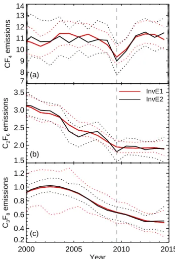
7 8 9 10 11 12 13 14 CF 4 emissions (a) 1.5 2.0 2.5 3.0 3.5 C2 F6 emissions InvE1 InvE2 (b) 2000 2005 2010 2015 Year 0.2 0.4 0.6 0.8 1.0 1.2 C3 F8 emissions (c)
Figure 8. (a) CF4, (b) C2F6and (c) C3F8emissions (Gg yr−1) from
2000 for the InvE1 inversion in red and the InvE2 inversion in black. Uncertainty ranges shown for both models are 95 % confidence in-tervals.
AGAGE 12-box model is not particularly well suited to this type of conclusion, and analysis with a model that has more accurate atmospheric transport, such as a 3-D atmospheric transport model, would be required to obtain a robust result. However, a general equatorward shift of a proportion of the emissions is consistent with the rapid rise of China into the aluminium market from the 1990s into the 2000s (Interna-tional Aluminium Institute, 2009, 2014) at a lower latitude on average than previous emissions based in North Amer-ica and Europe, for example in locations such as Canada and Norway (a map of the location of many aluminium smelters is shown in Wong et al. (2015), with a significant number of Chinese smelters south of 30◦N). The emergence of semi-conductor emissions in recent decades, with significant con-tributions of emissions from Asia, would also have caused an equatorward shift of a proportion of the emissions.
4.5 Global financial crisis (GFC)
Our study adds an extra 6 years of measurements compared to Mühle et al. (2010), extending the estimated emissions
to the end of 2014. Figure 8 shows the estimated emissions from both the InvE1 and InvE2 inversions for the three PFCs from 2000. Our best estimates for CF4emissions from both inversions varied mostly within the range 11 ± 0.5 Gg yr−1 between 1998 and 2007, before dropping by about 15 % in 2009, presumably due to reduced economic activity associ-ated with the GFC. CF4emissions in 2010 recovered some of this drop, then from 2011 to 2014 they varied about a mean level that was slightly higher than the 1998–2007 mean. The prior estimate for emissions growth rate used by the InvE1 inversion for CF4 was constant (i.e. assumes no emissions growth) from 2008, so the inferred dip must be due to the at-mospheric observations. Emissions of C2F6from the InvE2 inversion also show a dip in 2009, in addition to the al-ready decreasing trend between 1998 and 2007. The InvE1 inversion does not show a clear C2F6 dip. C2F6 emissions in both inversions were fairly steady from 2010. C3F8 emis-sions peaked about 2002, then decreased until 2012 and have been steady since. They do not seem to show an additional reduction around 2009 above the already decreasing trend, but both inversions have little interannual variability in their inferred emissions. The magnitude of the dip in the inferred emissions will be sensitive to the statistics of each inversion including data uncertainties and regularisation, although we see that the CF4 dip barely changes with the choice of the regularisation parameter α in Fig. 5b. The growth rate of a trend curve with 650 day smoothing fitted to Mace Head monthly PFC mole fraction shows pronounced dips in 2009 in CF4and C3F8but only a small dip in C2F6.
Global emissions of CO2 show a dip in 2009 due to
the GFC (Friedlingstein et al., 2010), followed by a rapid recovery (Peters et al., 2012), although the dip was only around 1.4 % and was dominated by emissions in developed countries and offset by increases in emissions in developing countries. Estimates of global primary aluminium production from the International Aluminium Industry show a 6 % re-duction in 2009 compared to 2008, dominated by developed countries but with steady levels from China. The price of pri-mary aluminium dropped by more than half from 2008 to 2009 (Barber and Tabereaux, 2014). Kim et al. (2014) (also shown in Wong et al., 2015) showed global top-down and bottom-up emissions estimated to 2010, and they have dips at the time of the GFC in the top-down estimates as well as both the aluminium and semiconductor components of the bottom-up emissions, but they were not specifically dis-cussed nor related to the GFC. The 2009 dip in bottom-up CF4emissions given by Kim et al. (2014) is 23 % for both aluminium and semiconductor emissions and 24 and 26 % in bottom-up aluminium and semiconductor C2F6emissions, respectively.
4.6 Recent years
While the initial reduction of PFC emission factors last century was a consequence of measures to reduce elec-tricity consumption during aluminium production, in recent decades there has been a concerted effort by both the alu-minium and semiconductor industries to reduce PFC emis-sions. However, the rate of decrease of emissions appears to have slowed and possibly stopped in recent years. Other than the 2009 dip, CF4 emissions have been quite steady since about 1998, C2F6 emissions have been steady since about 2010 and the decline in C3F8emissions appears to have re-cently stopped. Primary aluminium production has increased year after year and at a greater rate from the year 2000, so steady emissions imply decreasing emission factors. How-ever, due to the very long lifetimes of these gases, PFCs emit-ted become effectively a permanent part of the atmosphere and therefore make an enduring contribution to radiative forcing. The long lifetimes, together with their exceptionally high global warming potentials, underpin the urgent need for continued reduction of PFC emissions from all PFC generat-ing industries. This should involve further mitigation efforts by the two major emitting industries (aluminium and semi-conductors) and better quantification of emissions and (if necessary) mitigation efforts for the other potential sources (e.g. HCFC/fluorochemical production and rare earth indus-tries).
5 Summary and conclusions
We have reconstructed emissions and atmospheric abun-dance of CF4, C2F6and C3F8from 19th century levels (prior to anthropogenic influence) to 2014, using measurements from four firn sites, two ice cores and archived and in situ at-mospheric air from both hemispheres. We also inferred emis-sion factors for PFC emisemis-sions due to aluminium production prior to the 1980s. These are the first continuous records of PFC mole fraction and emissions from pre-anthropogenic to recent times. They demonstrate how unintended conse-quences of human actions and deliberate mitigation efforts have affected these important atmospheric constituents over the past century.
The 19th century levels of CF4were stable at 34.1±0.3 ppt and below detection limits of 0.002 and 0.01 ppt for C2F6and C3F8. CF4and C2F6both show peaks in emissions around 1940, presumably due to increased demand for aluminium production during World War II. These peaks are about at the limit of the time resolution recoverable from ice core and firn measurements. We estimate emission factors in 1940 of 2.2–4.8 kg t−1for CF4, 0.38–0.53 kg t−1for C2F6and 0.003– 0.04 kg t−1for C3F8.
At the recent end of the record, we see temporary reduc-tions in CF4(and perhaps C2F6) emissions in 2009, presum-ably associated with the impact of the GFC on global
alu-minium and semiconductor production. The strong decrease in PFC emissions that we have seen since the peaks in 1980 (CF4) and early-to-mid-2000s (C2F6 and C3F8) appears to have slowed and possibly stopped in recent years. Continued effort from all PFC generating industries is urgently needed to reduce the emissions of these potent greenhouse gases, which, once emitted, will stay in the atmosphere essentially permanently (on human timescales) and contribute to radia-tive forcing.
6 Data availability
The firn, ice core and archive PFC measurements and the reconstructed histories of mole fraction, emissions and emission factor are available in the Supplement. The in situ measurements are available on the CDIAC website doi:10.3334/CDIAC/atg.db1001.


![[PDF] Cours d'introduction aux normes du langage XHTML | Télécharger PDF](data:image/gif;base64,R0lGODlhAQABAIAAAP///wAAACH5BAEAAAAALAAAAAABAAEAAAICRAEAOw==)