HAL Id: hal-01741277
https://hal.inria.fr/hal-01741277
Submitted on 22 Mar 2018
HAL is a multi-disciplinary open access
archive for the deposit and dissemination of sci-entific research documents, whether they are pub-lished or not. The documents may come from teaching and research institutions in France or abroad, or from public or private research centers.
L’archive ouverte pluridisciplinaire HAL, est destinée au dépôt et à la diffusion de documents scientifiques de niveau recherche, publiés ou non, émanant des établissements d’enseignement et de recherche français ou étrangers, des laboratoires publics ou privés.
On distance-preserving elimination orderings in graphs:
Complexity and algorithms
David Coudert, Guillaume Ducoffe, Nicolas Nisse, Mauricio Soto
To cite this version:
David Coudert, Guillaume Ducoffe, Nicolas Nisse, Mauricio Soto. On distance-preserving elimination orderings in graphs: Complexity and algorithms. Discrete Applied Mathematics, Elsevier, 2018, 243, pp.140-153. �10.1016/j.dam.2018.02.007�. �hal-01741277�
On distance-preserving elimination orderings in graphs:
complexity and algorithms
∗David Coudert1, Guillaume Ducoffe2,3, Nicolas Nisse1, and Mauricio Soto4
1
Universit´e Cˆote d’Azur, Inria, CNRS, I3S, France
2ICI – National Institute for Research and Development in Informatics, Romania 3The Research Institute of the University of Bucharest ICUB
4
Departamento de Ingeniera Matem`atica, Universidad de Chile. Facultad de Ciencias Fsicas y Matem`aticas
Abstract
For every connected graph G, a subgraph H of G is isometric if the distance between any two vertices in H is the same in H as in G. A distance-preserving elimination ordering of G is a total ordering of its vertex-set V (G), denoted (v1, v2, . . . , vn), such that any subgraph
Gi= G\(v1, v2, . . . , vi) with 1 ≤ i < n is isometric. This kind of ordering has been introduced by
Chepoi in his study on weakly modular graphs [11]. We prove that it is NP-complete to decide whether such ordering exists for a given graph — even if it has diameter at most 2. Then, we prove on the positive side that the problem of computing a distance-preserving ordering when there exists one is fixed-parameter-tractable in the treewidth. Lastly, we describe a heuristic in order to compute a distance-preserving ordering when there exists one that we compare to an exact exponential time algorithm and to an ILP formulation for the problem.
Keyword: distance-preserving elimination ordering; metric graph theory; NP-complete; exact exponential algorithm; integer linear programming; bounded treewidth.
1
Introduction
Elimination orderings of a graph are total orderings of its vertex-set. Many interesting graph problems can be specified in terms of the existence of an elimination ordering with some given properties. These range from some practical problems in molecular biology and chemistry [8] to the analysis of graph search algorithms [14], the characterization of some graph classes [10, 29], and the study of network clustering methods in social networks [26]. On the computational point of view, vertex ordering characterizations of a given graph class often lead to efficient (polynomial-time) recognition algorithms for the graphs in this class [2, 6, 15, 21, 28]. In this work we will consider one specific kind of elimination ordering that is called distance-preserving elimination ordering [11]. Precisely, let us remind that a subgraph H of a graph G is isometric if the distance between any two vertices in H is the same in H as in G. An elimination ordering (v1, v2, . . . , vn)
of G is distance-preserving if it satisfies that each suffix (vi, vi+1, . . . , vn) with i < n induces an
isometric subgraph of G.
∗
This work has been supported by ANR project Stint under reference ANR-13-BS02-0007, ANR program “Invest-ments for the Future” under reference ANR-11-LABX-0031-01, and the Inria associated team AlDyNet.
Distance-preserving elimination orderings encompass several other elimination orderings stud-ied in the literature [6,7, 19, 24, 25, 28], all of which can be computed in polynomial time when they exist. In particular, known refinements of distance-preserving elimination orderings comprise the perfect elimination orderings [28], maximum neighbourhood orderings [6], h-extremal order-ings [7], semisimplicial elimination orderings [24], dismantlable orderings [25] and more generally domination elimination orderings [19]. The latter orderings characterize chordal graphs, dually chordal graphs, homogeneously orderable graphs, cop-win graphs and a subclass of tandem-win graphs [12] respectively, and as above stated they all can be computed in polynomial-time when they exist. However the complexity of deciding whether a distance-preserving elimination ordering exists in a given graph has been left open until this paper. We aim at completing the picture and characterizing the complexity of this problem.
Related work In [17] it has been proved that every graph with a distance-preserving elimination ordering has a minimum-size cycle basis with only triangles and quadrangles, that can be easily computed if a distance-preserving elimination ordering is part of the input. This property has been useful in the study of some tree-likeness invariants of graphs (e.g., in comparing treewidth with treelength). However, the complexity of recognizing graphs with a distance-preserving elimination ordering has been left open in [17]. Prior works [9, 11] have focused on the existence of distance-preserving elimination orderings in some well-structured graph classes, i.e., the weakly modular graphs. In particular, it has been proved recently in [9] that every breadth-first search ordering of a weakly modular graph is distance-preserving, that allows to compute one such ordering in linear time for a given graph in this class.
On the positive side, above stated refinements of distance-preserving elimination orderings [6,
7,19,24,25,28] can all be computed with greedy algorithms when they exist. Indeed, for all these orderings it can be tested in polynomial-time whether a given vertex can be eliminated first. As an example, any dominated vertex can be the starting vertex of some domination elimination ordering (total ordering of the vertex-set where for every suffix, the closed neighbourhood of the first vertex is dominated in the subgraph induced by the suffix). The latter implies that any partial domination elimination ordering can be extended unless the graph does not admit such a total order. A first hint that computing a distance-preserving elimination ordering can be more difficult is that it is not that simple to choose a starting vertex. For instance, consider the wheel W5 obtained from
a cycle C5 of length five by adding a universal vertex. Every elimination ordering of W5 where
the universal vertex is the last vertex eliminated is distance-preserving. However, if the universal vertex is eliminated first then the cycle C5 is an isometric subgraph of W5 that does not admit a
distance-preserving elimination ordering. The above problem occuring with C5 also occurs with
hypercubes, that can be proved using tools from discrete geometry1.
Our contributions We prove on the negative side that it is NP-complete to decide whether a given graph admits a distance-preserving elimination ordering (Section 3). The latter result may look surprising since as above stated, a broad range of distance-preserving orderings with additional properties can be computed in polynomial time when they exist. Then we show that the
1
More precisely, for the special case of an n-dimensional hypercube, the distance-preserving orderings are equivalent to the so-called “shellable orderings” as defined in [32]. In particular, if every partial distance-preserving ordering of the n-dimensional hypercube could be extended, then it would imply that its dual, the n-dimensional octahedron, is extendably shellable, that is known to be false for n ≥ 12 [22].
problem remains NP-complete even for general graphs with diameter at most two (Section 3.3). Note that in a sense our result is optimal w.r.t. the diameter because complete graphs trivially admit a distance-preserving ordering. Our reduction will show how to encode a 3-SAT formula in a graph whose distance-preserving orderings are in many-to-many correspondance with the satisfying assignments for the formula. This line of work resembles to the one in [31] in order to show that it is NP-complete to recognize collapsible complexes. Our work differs from theirs in that we study orderings with very distinct properties and the “simpler” structure of graphs —w.r.t. complexes— further constrains our gadgets to mimic variables and clauses of the formula.
On a more positive side, we prove in Section 4 that the problem of computing a distance-preserving ordering when there exists one is fixed-parameter-tractable in the treewidth.
Next, we show that a meta-theorem on vertex-orderings [3] can be applied to our problem, that results in an algorithm with O∗(2n)-time and space complexity, as well as in an algorithm with O∗(4n)-time and polynomial space complexity. We also propose an Integer Linear Programming formulation which may lead to a better running time in practice. These exact algorithms are described in Section 5as well as simple heuristic algorithms.
Notations Graphs in this study are finite, simple (hence without loop nor multiple edges) and unweighted. We refer to [5, 20] for standard reference books on graphs (see also [1] for a survey about metric graph theory). Let (v1, v2, . . . , vn) be an elimination ordering of a graph G, we say
that vertex vi, 1 ≤ i ≤ n, is the ith vertex to be eliminated, and that vertex vi is eliminated before
vertex vj, denoted vi≺ vj, if i < j.
2
Local characterization
In what follows, we will avoid considering all the distances in the graph at each time a vertex is eliminated. That is, we replace the “global” condition that G \ v is isometric by a “local” one implying only the neighbours of v. The following characterization will explain how to do so. Lemma 1. Let G = (V, E) and v ∈ V , the subgraph G \ v is isometric if and only if every two non-adjacent neighbours of vertex v have at least two common neighbours in G (including v). Proof. If G \ v is isometric, then let x, y ∈ NG(v) be non-adjacent. Since dG\v(x, y) = dG(x, y) = 2,
x and y have another common neighbour than vertex v. Conversely, suppose that every two non-adjacent neighbours of vertex v have at least two common neighbours in G. In particular, every of them have at least one common neighbour in G \ v. Then, for every two non-adjacent x, y ∈ NG(v)
the subpath (x, v, y) can be substituted in any shortest-path of G with the subpath (x, u, y) of G \ v, where u denotes a common neighbour of x, y. This proves that G \ v is an isometric subgraph.
By using Lemma1, one obtains the following characterization of distance-preserving elimination orderings. It can be seen as a reformulation of the characterization given in [11, Lemma 3.2] in terms of pseudopeakless functions.
Corollary 2. An elimination ordering ≺ of G = (V, E) is distance-preserving if and only if for every u, v ∈ V at distance dG(u, v) = 2, there is w ∈ NG(u) ∩ NG(v) such that u ≺ w or v ≺ w.
Proof. Let (v1, v2, . . . , vn) be the elimination ordering we consider. For every 0 ≤ i < n, define
Gi = G \ {v1, . . . , vi−1} (in particular G0 = G). On the one direction, suppose that ≺ is
Gi is an isometric subgraph of G. Hence, since vi, vj ∈ V (Gi) and dG(vi, vj) = 2, there exists
w ∈ NG(vi) ∩ NG(vj) such that w ∈ V (Gi), i.e., vi ≺ w. On the other direction, suppose that
≺ is not distance-preserving. Let i ≥ 0 be the least index such that Gi is an isometric subgraph
of G but Gi+1 = Gi \ vi is not. By Lemma 1, there exist x, y ∈ NGi(vi) nonadjacent such that
NGi(x) ∩ NGi(y) ∩ V (Gi+1) = ∅. In particular, there does not exist any w ∈ NG(x) ∩ NG(y) such
that x ≺ w or y ≺ w (else, w ∈ V (Gi+1)).
Finally, it may be easier sometimes to group vertices into subsets whose vertices can be elim-inated in an arbitrary way. On such occasions, we will base on the following consequence of Lemma1.
Corollary 3. Let G be a graph, S ⊂ V (G) satisfy that for every v ∈ S, every two non-adjacent neighbours of vertex v have a common neighbour in G \ S. Then, for any S0 ⊆ S, the subgraph G \ S0 is isometric.
Proof. By contradiction, let S0 ⊆ S falsify the corollary with S0 being of minimum size w.r.t. this property. Let v ∈ S0, S00 := S0 \ v. The subgraph G \ S00 is isometric by the minimality of S0. Furthermore, by the hypothesis every two non-adjacent neighbours of v have a common neighbour in G \ S, hence in G \ S0 so, G \ S0 is isometric by Lemma 1. This contradicts the fact that S0 falsifies the corollary.
3
Hardness results
The purpose of this section is to prove the following result.
Theorem 4. Deciding whether a given graph G admits a distance-preserving elimination ordering is NP-complete, already if G has diameter at most two.
Note that since the all-pairs-shortest-paths in a graph can be computed in polynomial-time then it easily follows that the problem is in NP and so, we will only prove the NP-hardness. We will first prove that deciding whether a given graph G admits a distance-preserving elimination ordering is NP-hard, already if G has diameter at most five. This first part of the proof is involved and it is based on a technical reduction from 3-SAT, the standard NP-complete problem [13]. Then, we will show how to lower the diameter to two (Section3.3).
3.1 Main reduction
Given a formula Φ with n variables and m clauses of exactly three literals each, the 3-SAT problem aims at deciding whether there exists a boolean assignment of the variables which makes the formula true. In case it does, then the formula Φ is said satisfiable. We will construct a graph GΦ from an
arbitrary formula Φ so that there is a distance-preserving elimination ordering of GΦ if and only
if Φ is satisfiable. This will prove the NP-hardness of our problem. To achieve the result, assume w.l.o.g. that no litteral and its negation can be contained in the same clause of Φ (else, any such clause could be removed from Φ), and every variable appears both positively and negatively in the clauses of Φ (else, any clause containing either this variable or its negation could also be removed from Φ). Let us denote by x1, x2, . . . , xn the n variables, and by C1, C2, . . . , Cm the m clauses of
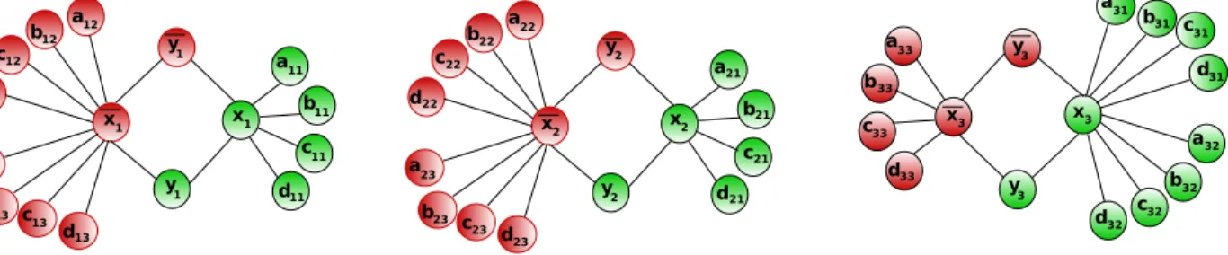
Variable gadget For every variable xi, 1 ≤ i ≤ n, let us add in GΦ an induced quadrangle
(xi, yi, ¯xi, ¯yi) (i.e., a cycle with four vertices). For every 1 ≤ j ≤ m, if xi is in the jth clause of the
formula then four more vertices aij, bij, cij, dij are added and made adjacent to vertex xi. Similarly
if ¯xi is in the jth clause of the formula then four more vertices aij, bij, cij, dij are added and made
adjacent to vertex ¯xi (this is clearly defined because no clause contains both literals xi, ¯xi by the
hypothesis). We refer to Figure1 for an illustration.
x1 x1 y1 y1 12 b d11 c12 a12 c11 a11 b11 d12 a13 b13 c13 d13 x2 x2 y2 y2 23 a b21 a21 c21 d21 c22 c23 b22 a22 b23 d22 d23 x3 x3 y3 y3 31 d c31 c32 b32 b31 a31 d32 a32 a33 d33 b33 c33
Figure 1: The three variable gadgets for the formula Φ = (x1∨x2∨x3)∧( ¯x1∨ ¯x2∨ ¯x3)∧( ¯x1∨ ¯x2∨x3).
To better understand the role played by the quadrangle (xi, yi, ¯xi, ¯yi) in our reduction, we make
the following observation that captures well the difficulty of the problem. Indeed, every vertex in a quadrangle can be chosen as the starting vertex of a distance-preserving ordering. However, the vertex diametrically opposed cannot be chosen as the second vertex to be eliminated. We will make use of a similar trick in our reduction so as to mimic a truth table with variable gadgets, ensuring that the second vertex to be eliminated in xi, ¯xi must be eliminated after one of each pair xi0, ¯xi0
has already been eliminated for any 1 ≤ i0 ≤ n.
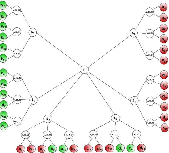
Clause tree Second, a rooted tree of depth two with 8m + 1 vertices is added in GΦ. More
precisely, the tree is rooted at some newly added vertex rΦ that has 2m children denoted by
s1, t1, s2, t2, . . . , sm, tm. Informally, for every 1 ≤ j ≤ m both nodes sj, tj represent the jth clause
of Φ. Moreover let Cj = lp∨ lq∨ lrwith p < q < r and li ∈ {xi, ¯xi} for every i ∈ {p, q, r}. Then, the
internal node sj has three children denoted by uj(p, q), uj(q, r) and uj(r, p), similarly the internal
node tj has three children denoted by vj(p, q), vj(q, r) and vj(r, p). Finally, let us describe how the
clause tree is linked to the variable gadgets. Precisely, any leaf node uj(p, q) is made adjacent to
the pair of vertices apj, bqj, and in the same way any leaf node vj(p, q) is made adjacent to the pair
of vertices cpj, dqj. We refer to Figure 2for an illustration.
Our reduction will ensure that rΦis the unique common neighbour of sj, tj in GΦ. Consequently,
by Corollary 2 in any distance-preserving ordering of GΦ one of sj, tj will need to precede vertex
rΦ. We will show that this implies that the jth clause of Φ is satisfied.
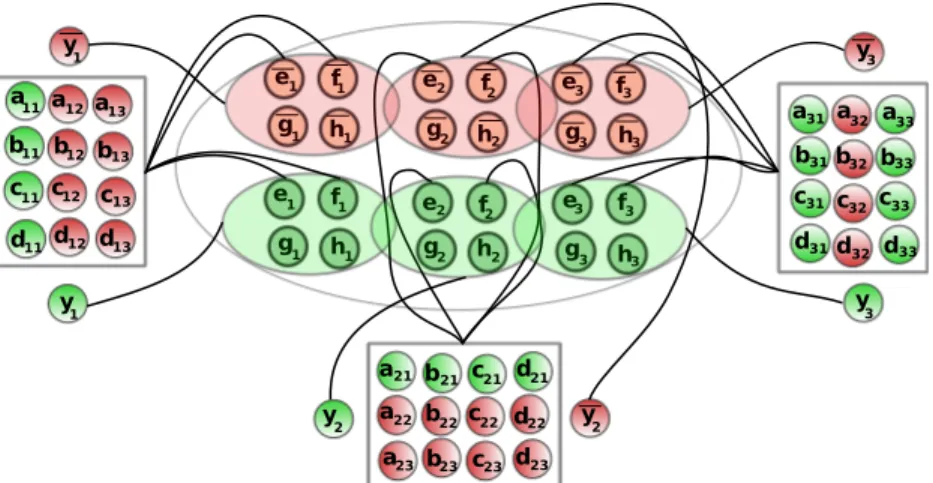
Literal clique The final and most technical part of our reduction is to construct a clique of GΦ
with 8n vertices so as to ensure that a distance-preserving ordering exists if Φ is satisfiable. For every 1 ≤ i ≤ n, the clique contains four vertices denoted by ei, fi, gi, hi (related to variable xi). In
the same way there are four vertices denoted by ¯ei, ¯fi, ¯gi, ¯hi (related to the negated variable ¯xi).
This clique is connected to variable gadgets as follows. Vertex yi (in the ith variable gadget)
is made adjacent to each of the four vertices ei, fi, gi, hi, and in the same way vertex ¯yi is made
s t s t s t 1 1 2 2 3 3 u (1,2)1 u(3,1)1 u (2,3)1 r a a a a a a a a a b b b b b b b b b c c c c c c c c c d d d d d d d d d 11 11 11 11 21 21 21 21 31 31 31 31 12 12 12 12 22 22 22 22 32 32 32 32 13 13 13 13 23 23 33 33 23 23 33 33 v (1,2)1 v (2,3)1 v(3,1)1 v (3,1)2 v (2,3)2 v (1,2)2 u (3,1)2 u (2,3)2 u (1,2)2 v (3,1)3 v (2,3)3 v (1,2)3 u (1,2)3 u (2,3)3 u (3,1)3
Figure 2: The clause tree for the formula Φ = (x1∨ x2∨ x3) ∧ ( ¯x1∨ ¯x2∨ ¯x3) ∧ ( ¯x1∨ ¯x2∨ x3).
literal of Cj, the four vertices aij, bij, cij and dij are made adjacent to each of the four vertices ei, fi
and ¯ei, ¯fi.
Then, the clique is connected to the clause tree as follows. For any 1 ≤ j ≤ m, let Cj = lp∨lq∨lr
with p < q < r and li ∈ {xi, ¯xi} for every i ∈ {p, q, r}, then:
• the three vertices uj(p, q), uj(q, r), uj(r, p) are respectively made adjacent to the 4-tuples of
vertices: (ep, gp and ¯eq, ¯gq); (eq, gq and ¯er, ¯gr); (er, gr and ¯ep, ¯gp);
• similarly, the three vertices vj(p, q), vj(q, r), vj(r, p) are respectively made adjacent to the
4-tuples of vertices: (fp, hp and ¯fq, ¯hq); (fq, hq and ¯fr, ¯hr); (fr, hr and ¯fp, ¯hp);
• last, vertex sj is made adjacent to the twelve vertices ei, gi and ¯ei, ¯gi with i ∈ {p, q, r};
similarly, vertex tj is made adjacent to the twelve vertices fi, hi and ¯fi, ¯hi with i ∈ {p, q, r}.
Let E = [ 1≤i≤n {ei, ¯ei}, F = [ 1≤i≤n {fi, ¯fi}, G = [ 1≤i≤n {gi, ¯gi} and H = [ 1≤i≤n {hi, ¯hi} partition the
clique. The root vertex rΦ of the clause tree is made adjacent to every vertex in G ∪ H. We refer
e f g h e e e e e f f f f f g g g g g h h h h h 1 2 3 3 3 3 3 3 3 3 2 2 2 2 2 2 2 1 1 1 1 1 1 1 a b c d a a b b a a a b b b b b b c c c c c c c c d d d d d d d d 11 12 13 21 22 23 31 32 33 11 11 11 12 12 12 13 13 13 21 21 21 22 22 22 23 23 23 31 31 31 32 32 32 33 33 33 a a a y y y y y y 1 2 3 3 2 1
(a) Adjacency relations between vertices from the variable gadgets and those from the literal clique.
r s t a b c d e e f f g g h h x x y y u(1,2)3 u(3,1)3 v(1,2)3 v(3,1)3 3 3 1 1 1 1 3 3 3 3 1 1 1 1 1 1 1 1 1 1 1 1
(b) Adjacency relations w.r.t. literal ¯x1 and clause C3= ¯x1∨ ¯x2∨ x3.
Figure 3: The literal clique, for the formula Φ = (x1∨ x2∨ x3) ∧ ( ¯x1∨ ¯x2∨ ¯x3) ∧ ( ¯x1∨ ¯x2∨ x3).
The resulting graph GΦ has diameter at most five. Indeed, all vertices but the xi, ¯xi with
1 ≤ i ≤ n are adjacent to the literal clique, therefore it is a 2-distance dominating clique. We will show later how to lower the diameter (Section3.3). Note that several vertices play almost identical roles in the reduction. This redundancy is necessary in order to ensure that most pairs of vertices that are at distance two in GΦ only have one common neighbour. Indeed, the latter will impose
3.2 Proof of correctness
We are now ready to prove that it is NP-hard to decide whether a given graph G admits a distance-preserving elimination ordering. We divide the proof in two propositions, as follows.
Proposition 5. If Φ is satisfiable, then GΦ admits a distance-preserving ordering.
Proof. Let us fix a boolean assignment of the variables xisatisfying Φ, that exists by the hypothesis.
In particular, let {li, ¯li} = {xi, ¯xi} be such that li is true, let V0 = {¯li | 1 ≤ i ≤ n} and let
V1 = {li | 1 ≤ i ≤ n}. Now, consider the following partition of the vertex-set of GΦ into eleven
subsets Sk, with 1 ≤ k ≤ 11. Let G0 := GΦ, and let Gk := Gk−1\ Sk for every 1 ≤ k < 11. We
will exhibit from the partition a distance-preserving ordering of GΦ. Precisely, we will prove that
for every 1 ≤ k ≤ 11 and for any total ordering Sk0 of Sk, the elimination ordering S10, S 0 2, . . . , S
0 11is
distance-preserving.
The partition is defined as follows:
• The variable gadgets are partitioned into five subsets S1, S2, S7, S8, S9. Furthermore, S1 =
V1 = {li | 1 ≤ i ≤ n}, S8 = V0 = {¯li | 1 ≤ i ≤ n}, S7 =
[
1≤i≤n
{yi, ¯yi}. The subsets S2, S9
contain the vertices aij, bij, cij, dij that are respectively adjacent to a vertex of V1, V0.
• The clause tree is partitioned into four subsets S3, S4, S5, S10. Furthermore, S5 = {rΦ}, S4=
{s1, t1, s2, t2, . . . , sm, tm}. The subset S3 contains the vertices uj(p, q), vj(p, q) such that the
jth clause is satisfied by one of lp, lq ∈ V1; similarly, the subset S10 contains the vertices
uj(p, q), vj(p, q) such that the jth clause is neither satisfied by lp nor lq.
• The literal clique is partitioned into two subsets S6 = G ∪ H and S11= E ∪ F .
In what follows, we will prove that for every 1 ≤ k ≤ 11, the pair hGk−1, Ski satisfies the
sufficient condition of Corollary3. The latter will prove, as claimed above, that for every 1 ≤ k ≤ 11 and for any total ordering Sk0 of Sk, the elimination ordering S10, S20, . . . , S110 is distance-preserving.
• Let S1 = V1 = {li | 1 ≤ i ≤ n}. Let li ∈ S1. Neighbours of li in G0 are yi, ¯yi and every of
aij, bij, cij, dij such that li∈ Cj. Let α, β ∈ NG0(li) be non-adjacent. There are four subcases.
– if {α, β} = {yi, ¯yi} then ¯li is a common neighbour of α, β;
– if one of α, β is equal to yi and the other is amongst aij, bij, cij, dij for some j, then ei, fi
are common neighbours of α, β;
– similarly, if one of α, β is equal to ¯yi and the other is amongst aij, bij, cij, dij for some j,
then ¯ei, ¯fi are common neighbours of α, β;
– if α is amongst aij, bij, cij, dij for some j, and β is amongst aij0, bij0, cij0, dij0 for some j0,
then ei, fi and ¯ei, ¯fi are common neighbours of α, β.
Therefore, in all cases α, β have a common neighbour in G1, and Corollary3applies. In other
words, G1 = GΦ\ S1 is isometric and for every total ordering S10 of S1, for any prefix S100 of
• Let S2 contain every aij, bij, cij, dij such that clause Cj is satisfied by li. Let w ∈ S2. There
exist j ≤ m, p < q < r ≤ n such that neighbours of w in G1 are composed of ep, fp, ¯ep, ¯fp
and one of uj(p, q), uj(r, p), vj(p, q) or vj(r, p). Let α, β ∈ NG1(w) be non-adjacent. Note
that w has only one neighbour in G1 that is not in the literal clique. Consequently, one
of α, β is amongst uj(p, q), uj(r, p), vj(p, q), vj(r, p). Since the latter four vertices have some
neighbour in the literal clique by construction, therefore α, β have a common neighbour in G2 and Corollary 3 applies. In other words, G2 = G1\ S1 is isometric and for every total
ordering S20 of S2, for any prefix S200 of S02, G1\ S200 is isometric.
• Let S3 contain uj(p, q), vj(p, q) for every j ≤ m and p, q ≤ n such that one of lp, lq satisfies
clause Cj. Let w ∈ S3. There exist j ≤ m, p, q ≤ n such that either w = uj(p, q) or
w = vj(p, q). Two cases thus need to be distinguished:
– Case w = uj(p, q). In particular, the neighbours of w in G2 are sj, ep, gp, ¯eq, ¯gq and
at most one amongst apj, bqj. Furthermore, let α, β ∈ NG2(w) be non-adjacent. If
apj∈ NG2(w) then α, β ∈ NG2[ep], otherwise α, β ∈ NG2[ ¯eq].
– Case w = vj(p, q). In particular, the neighbours of w in G2 are tj, fp, hp, ¯fq, ¯hq and
at most one amongst cpj, dqj. Furthermore, let α, β ∈ NG2(w) be non-adjacent. If
cpj ∈ NG2(w) then α, β ∈ NG2[fp], otherwise α, β ∈ NG2[ ¯fq].
In both cases, any two non-adjacent neighbours α, β of w have a common neighbour in G3
and so, Corollary 3 applies. In other words, G3 = G2\ S3 is isometric and for every total
ordering S30 of S3, for any prefix S300 of S03, G2\ S300 is isometric.
• Let S4 = {s1, t1, s2, t2, . . . , sm, tm} be the vertices representing each clause. Let w ∈ S4.
Clearly, there exists j ≤ m such that either w = sj or w = tj. Furthermore, by the choice of a
boolean assignment satisfying Φ, there exists lp ∈ S1 satisfying Cj. Up to cyclic permutation
of the indices for the variables, this implies by construction uj(p, q), uj(r, p), vj(p, q), vj(r, p) ∈
S3 for some q, r > p. Two cases need to be distinguished.
– Case w = sj. In particular, the neighbours of w in G3 are rΦ, the twelve vertices
ei, gi, ¯ei, ¯gi with i ∈ {p, q, r}, and possibly uj(q, r). Recall that rΦ is adjacent to all
the vertices of G ∪ H, furthermore uj(q, r) is adjacent to eq, gq and ¯er, ¯gr. Therefore,
NG3(w) ⊆ N [gq] ∩ N [¯gr]. In this situation for any two non-adjacent neighbours α, β of
w in G3 we have α, β ∈ NG3[gq] (resp., α, β ∈ NG3[¯gr]).
Let us point out that in the full graph G, the two vertices uj(p, q) and uj(r, p) are
also neighbours of w = sj in G. Furthermore, by construction w is the unique common
neighbour of uj(p, q) and uj(r, p) in G. Hence, it is crucial that since Φ is satisfiable, and
so, Cj is satisfied by some literal lp, the two vertices uj(p, q) and uj(r, p) are eliminated
in S3.
– Case w = tj. In particular, the neighbours of w in G3 are rΦ, the twelve vertices
fi, hi, ¯fi, ¯hi with i ∈ {p, q, r}, and possibly vj(q, r). Recall that rΦ is adjacent to all
the vertices of G ∪ H, furthermore vj(q, r) is adjacent to fq, hq and ¯fr, ¯hr. Therefore,
NG3(w) ⊆ N [hq] ∩ N [¯hr]. In this situation for any two non-adjacent neighbours α, β of
w in G3 we have α, β ∈ NG3[hq] (resp., α, β ∈ NG3[¯hr]).
As before, let us point out that in the full graph G, the two vertices vj(p, q) and vj(r, p)
common neighbour of vj(p, q) and vj(r, p) in G. Hence, it is crucial that since Φ is
satisfiable, and so, Cj is satisfied by some literal lp, the two vertices vj(p, q) and vj(r, p)
are eliminated in S3.
In both cases, any two non-adjacent neighbours α, β of w have a common neighbour in G4.
By Corollary3, G4= G3\ S4 is isometric and for every total ordering S40 of S4, for any prefix
S400 of S40, G3\ S400 is isometric.
• Let S5 = {rΦ}. By construction the neighbourhood of rΦ in the full graph G is equal to
S4∪ G ∪ H. Note that for every j ≤ m, rΦ is the unique common neighbour of sj and tj in
G, hence G \ rΦ is not isometric. However, since all vertices in S4 have been eliminated at
this step, rΦ is simplicial in G4, i.e., its neighbourhood NG4(rΦ) = G ∪ H induces a complete
subgraph. It is thus straightforward that Corollary3 applies. In other words, G5 = G4\ rΦ
is isometric.
• Let S6 = G ∪ H. Let w ∈ S6. There are four cases to be considered.
– If w = gi for some i, then neighbours of gi in G5 are those in the literal clique, vertex yi
and every uj(i, q) /∈ S3. Therefore, NG5[w] ⊆ NG5[ei];
– if w = ¯gi for some i, then neighbours of ¯gi in G5 are those in the literal clique, vertex ¯yi
and every uj(p, i) /∈ S3. Therefore, NG5[w] ⊆ NG5[ ¯ei];
– if w = hi for some i, then neighbours of hi in G5 are those in the literal clique, vertex yi
and every vj(i, q) /∈ S3. Therefore, NG5[w] ⊆ NG5[fi];
– else, w = ¯hi for some i, hence neighbours of ¯hi in G5 are those in the literal clique,
vertex ¯yi and every vj(p, i) /∈ S3. Therefore, NG5[w] ⊆ NG5[ ¯fi].
Since, ei, ¯ei, fi, ¯fi ∈ V (G6), therefore Corollary 3 applies. In other words, G6 = G5 \ S6 is
isometric and for every total ordering S60 of S6, for any prefix S600 of S60, G5\ S600 is isometric.
• Let S7 contain yi, ¯yi for every 1 ≤ i ≤ n. Let w ∈ S7. There is some i such that neighbours
of w in G6 are vertex ¯li and either ei, fi (if w = yi) or ¯ei, ¯fi (if w = ¯yi). Moreover, recall that
we assume the existence of some 1 ≤ j ≤ m such that ¯li appears in clause Cj. Indeed, all
variables are assumed to appear positively and negatively in the clauses of Φ. In particular, by construction aij, bij, cij, dij ∈ S/ 2 and so, aij, bij, cij, dij ∈ V (G6). The latter four vertices
are adjacent to every of ¯li, ei, fi and ¯ei, ¯fi by construction of GΦ. As a result, for any
α, β ∈ NG6(w) non-adjacent, α, β have a common neighbour in G7 and so, Corollary 3
applies. In other words, G7 = G6\ S7 is isometric and for every total ordering S70 of S7, for
any prefix S700 of S07, G6\ S700 is isometric.
• Let S8 = V0 = {¯li | 1 ≤ i ≤ n}. Let ¯li ∈ S8. Neighbours of ¯li in G7 are those aij, bij, cij, dij
such that ¯li appears in Cj. Every such neighbour is adjacent to the 4-tuple ei, fi, ¯ei, ¯fi of the
literal clique, hence Corollary 3 applies. In other words, G8 = G7 \ S8 is isometric and for
every total ordering S80 of S8, for any prefix S800 of S 0
8, G7\ S800 is isometric.
• Let S9contain every aij, bij, cij, dijsuch that ¯liappears in Cj. The proof for this case is similar
as for S2. Let w ∈ S9. There are j ≤ m, p < q < r ≤ n such that neighbours of w in G8
are ep, fp, ¯ep, ¯fp and at most one of uj(p, q), uj(r, p), vj(p, q) or vj(r, p). Let α, β ∈ NG8(w) be
any other neighbour of w is in the literal clique. Furthermore, uj(p, q), uj(r, p), vj(p, q), vj(r, p)
are respectively adjacent to ep, er, fp, fr in the literal clique, that are part of E ∪ F and so,
have not been eliminated with S6. Therefore, α, β have a common neighbour in G9 and so,
Corollary3applies. In other words, G9 = G8\ S9 is isometric and for every total ordering S90
of S9, for any prefix S900 of S90, G8\ S900 is isometric.
• Let S10 contain every uj(p, q), vj(p, q) such that ¯lp, ¯lq appear in Cj. Equivalently, those are
all of uj(p, q), vj(p, q) but the ones already in S3. Let w ∈ S10. There exist j, p, q such that
neighbours of w in G9 are either ep, ¯eq (if w = uj(p, q)) or fp, ¯fq (if w = vj(p, q)). As a result,
vertex w is simplicial. It thus follows that Corollary 3 trivially applies. In other words, G10= G9\ S10 is isometric and for every total ordering S100 of S10, for any prefix S1000 of S
0 10,
G9\ S1000 is isometric.
• Finally, let S11 = E ∪ F , this is a clique and so, the vertices in S11 can be eliminated
sequentially while leaving a sequence of isometric subgraphs.
To sum up, one obtains a distance-preserving ordering of GΦ by sequentially eliminating vertices
in S1 then in S2 and so on until S11, in an arbitrary way.
Proposition 6. If GΦ admits a distance-preserving elimination ordering, then Φ is satisfiable.
Proof. Let ≺ be a distance-preserving ordering of GΦ. For every 1 ≤ j ≤ m we claim that there
is 1 ≤ i ≤ n such that some li ∈ {xi, ¯xi} satisfies clause Cj, and li ≺ rΦ. Then, we will prove
that this implies a boolean assignment of the variables satisfying Φ by showing that rΦ≺ ¯li, where
{li, ¯li} = {xi, ¯xi}.
To prove the claim, first observe that for every 1 ≤ j ≤ m, rΦ is the unique common neighbour
of sj, tj in GΦ. By Corollary 2, it implies sj ≺ rΦ or tj ≺ rΦ. So, assume sj ≺ rΦ (the case tj ≺ rΦ
is symmetrical to this one). Let uj(p, q), uj(q, r), uj(r, p) be the three children of sj in the clause
tree. Note that the latter three vertices pairwise share sj as their unique common neighbour in
GΦ. Consequently, by Corollary2 (applied twice) at least two of them must be eliminated before
sj. W.l.o.g., let uj(p, q) be eliminated before sj. In such case, note that uj(p, q) is the unique
common neighbour of apj, bqj by construction of GΦ. Therefore, by Corollary 2, apj ≺ uj(p, q) or
bqj ≺ uj(p, q). Suppose by symmetry that apj ≺ uj(p, q). Let lp ∈ {xp, ¯xp} appear in Cj. Since
lp and uj(p, q) share apj as their unique common neighbour and apj ≺ uj(p, q), by Corollary 2
lp ≺ apj ≺ rΦ, that finally proves the claim.
To conclude let us prove for every 1 ≤ i ≤ n, there is li ∈ {xi, ¯xi} such that either li ≺ rΦ≺ ¯li
or rΦ ≺ li ≺ ¯li. If so, then let us consider any boolean assignment of the variables satisfying for
every 1 ≤ i ≤ n, li is assigned true if li ≺ rΦ (note that if rΦ ≺ li ≺ ¯li, then xi can be valuated
in an arbitrary way). Since by the above claim, for every 1 ≤ j ≤ m, there is li ≺ rΦ satisfying
clause Cj, therefore any such assignment satisfies the formula Φ. By way of contradiction, suppose
li ≺ ¯li ≺ rΦ with {li, ¯li} = {xi, ¯xi} for some 1 ≤ i ≤ n. Since yi, ¯yi share xi, ¯xi as their only two
common neighbours in GΦ, by Corollary2 yi ≺ ¯li or ¯yi ≺ ¯li. Suppose by symmetry yi≺ ¯li. Then,
since yi is the unique common neighbour between ¯li and gi, hi, we have by Corollary 2that gi ≺ yi
and hi ≺ yi. However, we claim that the combination of gi ≺ yi ≺ rΦ and hi≺ yi≺ rΦ contradicts
the fact that ≺ is distance-preserving. Indeed, gi, hi are the only two common neighbours of rΦ
3.3 Reduction to graphs with diameter at most two
As stated before, the graph GΦresulting from our reduction in Section3.1has diameter at most five.
In this section, we improve the result by lowering the diameter to two, thereby proving Theorem4. We base on the local view of Corollary 2, which states that in order to obtain a distance-preserving ordering of G it is necessary and sufficient to ensure that vertices at distance two in G still have a common neighbour in the graph at each time a vertex is eliminated. This motivates the following Definition 7 — to embed any graph G into a graph G0 with diameter at most two such that any two vertices at distance two in G have the same set of common neighbours in G and G0. Definition 7. Let G be a connected graph with n vertices, let H = {{u, v} | u, v ∈ V (G) and dG(u, v) ≥
3} and let p = |H|. The graph G0is obtained from G by adding a clique Z of n + p vertices, defined as follows.
For every vertex v ∈ V (G), there is zv ∈ Z that is adjacent to v in V (G).
For every u, v ∈ V (G) such that dG(u, v) ≥ 3, i.e., {u, v} ∈ H, there is zuv ∈ Z that is adjacent
to u, v in V (G).
Lemma 8. For any connected graph G, let G0 be as in Definition7, G0 has diameter at most two. Proof. Let u, v ∈ V (G0). If u ∈ Z or v ∈ Z then dG0(u, v) ≤ 2 because either u, v ∈ Z are adjacent
or, w.l.o.g., u ∈ Z and zv ∈ Z is a common neighbour of u, v in G0 by Definition7. Else, u, v ∈ V (G)
and so, dG0(u, v) ≤ dG(u, v) because G is an induced subgraph of G0. Moreover, if dG(u, v) ≥ 3
then by Definition7 there is zuv∈ Z adjacent to u, v in G0, therefore dG0(u, v) = 2.
Lemma 9. For any connected graph G, let G0 be as in Definition7, G admits a distance-preserving ordering if and only if G0 admits one.
Proof. Let (v1, v2, . . . , vn) be a distance-preserving ordering of G. For every 1 ≤ i < n, let Gi :=
G\(v1, . . . , vi) be an isometric subgraph of G, let G0ibe the subgraph of G
0induced by V (G
i)∪Z (by
convention, G0:= G, G00 := G 0
). We claim that for every 1 ≤ i < n, G0i is an isometric subgraph of G0. Note that if the claim holds, then (v1, v2, . . . , vn) can be completed into a distance-preserving
ordering of G0 as follows: vertices v1, v2, . . . , vn are sequentially eliminated, then vertices of the
clique Z are eliminated in an arbitrary way2. To prove the claim, by Lemma1 it suffices to prove that any two x, y ∈ NG0
i−1(vi) non-adjacent share a common neighbour in G
0
i. If x, y ∈ V (Gi−1),
then by Lemma 1 they share a common neighbour in Gi, hence in G0i. Else, one of x, y is in Z,
w.l.o.g. say x ∈ Z and so, zy ∈ Z is a common neighbour of x, y in G0i.
Conversely, let G0 admit a distance-preserving ordering. Let ≺ be a distance-preserving elimi-nation ordering of G0, and let us consider the restriction (v1, v2, . . . , vn) of the total ordering ≺ to
the vertices of G. We claim that it is a distance-preserving elimination ordering of G. By contra-diction, let i be the least index such that Gi := G \ (v1, v2, . . . , vi) is not an isometric subgraph of
G (by convention, G0 := G). Let j be such that vi is the jth vertex to be eliminated in G0 w.r.t.
≺, and let G0j be obtained from G0 by removing the j first vertices to be eliminated in G0 w.r.t. ≺. Note that G0j is an isometric subgraph of G0 because ≺ is distance-preserving by the hypothesis. Moreover, since (v1, v2, . . . , vn) is assumed not to be distance-preserving, then by Lemma1, there
exist x, y ∈ NGi−1(vi) non-adjacent whose unique common neighbour in the subgraph Gi−1is vi. In 2
In fact, if vertices zv1, zv2, . . . , zvn are the last removed in Z then one obtains a breadth-first search ordering
rooted at zvn. This proves that the problem of deciding whether there exists a breadth-first search ordering that is
such case, dG(x, y) = 2, therefore x, y have no common neighbour in the clique Z by Definition 7.
However, V (Gi) ⊆ V (G0j) ⊆ V (Gi) ∪ Z by construction, therefore x, y have no common neighbour
in G0j, that contradicts the fact that G0j is an isometric subgraph of G0 by Lemma1. Altogether, we can now prove our main result as follows.
Proof of Theorem4. The problem is in NP. In order to prove the NP-hardness, let Φ be any instance for 3-SAT. The graph GΦ, described in Section3.1, can be constructed from Φ in polynomial time.
Furthermore, by the combination of Propositions5and6, GΦadmits a distance-preserving ordering
if and only if Φ is satisfiable. Finally, let G0Φ be obtained from GΦ as defined in Definition 7. By
Lemma8, G0Φhas diameter at most two, furthermore by Lemma9, G0Φadmits a distance-preserving ordering if and only if GΦ admits one, that is if and only if Φ is satisfiable. Since 3-SAT is
NP-complete [13], this proves the hardness and so, the result.
4
A polynomial case
In this section, we prove that the problem of computing a distance-preserving ordering when there exists one is fixed-parameter-tractable in the treewidth.
A tree-decomposition (T, X ) of a graph G = (V, E) is a pair consisting of a tree T and of a family X = (Xt)t∈V (T ) of subsets of V indexed by the nodes of T and satisfying:
(i) [
t∈V (T )
Xt= V ;
(ii) for any edge e = {u, v} ∈ E, there exists t ∈ V (T ) such that u, v ∈ Xt;
(iii) for any v ∈ V , {t ∈ V (T ) | v ∈ Xt} induces a subtree, denoted by Tv, of T .
The sets Xt are called the bags of the decomposition. Furthermore, the width of (T, X ) is equal to
max
t∈V (T )|Xt| − 1, and the treewidth of G is the minimum possible width of its tree-decompositions.
It is well-known that many NP-hard problems are fixed-parameter tractable (FPT) in the treewidth [18]. Furthermore, the existence of distance-preserving orderings has been proved useful in the comparative study of treewidth with some other properties of the tree-decompositions of graphs [17]. We prove that it can be decided in polynomial-time whether a given bounded treewidth graph admits a distance-preserving ordering, and if so, one such ordering can also be computed in polynomial-time. More precisely, we prove in what follows that the problem is FPT with the treewidth as parameter.
Theorem 10. For every G = (V, E) with treewidth at most k, it can be decided whether a distance-preserving ordering exists in time 22O(k) · nO(1). Furthermore, if it is the case, then a distance-preserving ordering for G can also be computed within the same amount of time.
Proof. For simplicity, we will work on a specific kind of decompositions, called nice tree-decompositions. A tree-decomposition (T, X ) is nice if T is rooted in some node r ∈ V (T ), any node of T has a at most two children and, for any t ∈ V (T ),
• or t has one child u and there exists v ∈ V such that Xt= Xu\ {v} (Forget Node);
• or t has one child u and there exists v ∈ V such that Xt= Xu∪ {v} (Introduced Node);
• or t has two children u and w and Xu = Xw = Xt (Join Node).
In what follows, let (T, X ) be a nice tree-decomposition of width O(k). It can be computed in time 2O(k)n [4]. For every t ∈ V (T ), let Tt be the subtree rooted at node t and let Vt =
[
u∈Tt
Xu. We
aim at computing all the orderings on Vtthat can be extended to a distance-preserving ordering of
G. In order to do so, we will represent an ordering on Vtas follows:
• its subordering ≺t on Xt;
• the collection Ctof pairs (N (v) ∩ Xt, posv) for every v ∈ Vt\ Xt, where posv is the number of
neighbours in N (v) ∩ Xt preceding vertex v;
• finally, a set Pt of pairs x, y ∈ Xt at distance two in G such that both x and y are preceded
by all their common neighbours in Vt.
Note that for any fixed vertex v ∈ Vt, there are 2O(k)possibilities for N (v)∩Xtand O(k) possibilities
for posv. In particular, since Ct can be any subset of a set with O(k)2O(k) elements, there are
2O(k)2O(k)possibilities for Ct. Overall there are k!·2O(k)2
O(k)
·O(k2) = 22O(k)possible representations. Intuitively, we aim at computing for every node t ∈ V (T ) the suborderings ≺tof Vtthat could
be potentially extended to a distance-preserving elimination ordering of G. In order to do so, let ≺ be any distance-preserving elimination ordering of G, let t ∈ V (T ) and let ≺tbe the subordering of
≺ constrained to Vt. By Corollary2, for every x, y ∈ Vtat distance two in G, there exists a common
neighbour z ∈ NG(x) ∩ NG(y) such that either x ≺ z or y ≺ z. Furthermore, if z ∈ Vtthen we have
either x ≺t z or y ≺tz, otherwise since z /∈ Vt we have by the properties of a tree-decomposition
that x, y ∈ Xt. Hence, we will consider a representation to be valid at node t ∈ V (T ) if it represents
an ordering ≺0t of Vt with the following property: for every x, y ∈ Vt at distance two in G, there
exists a common neighbour z ∈ NG(x) ∩ NG(y) such that either {x, y} ∈ Pt and z ∈ V \ Vt, or
z ∈ Vt and one of x or y precedes z w.r.t. ≺0t.
For every t ∈ V (T ), the following algorithm will compute all the valid representations at node t. Let us observe that for every subordering ≺tof Vt and for any child u ∈ V (T ) of t, if ≺thas a valid
representation at node t then its restriction ≺u to Vu also has a valid representation at node u.
We will use this observation in what follows in order to compute the valid representations at every node by dynamic programming. Furthermore, if ≺ is a distance-preserving ordering of G then as proved above, for every t ∈ V (T ) its restriction ≺t to Vt has a valid representation at node t.
Conversely, by Corollary 2 a valid representation at the root is equivalent to the existence of a distance-preserving ordering of G. Therefore, the valid representations at the root are exactly the representations of distance-preserving orderings of G, and so, the following algorithm is correct.
• Case of a Leaf Node. In this situation, Vt = Xt = {v} for some v ∈ V . So, there is a
unique valid representation (≺t= (v), Ct= ∅, Pt= ∅).
• Case of a Forget Node. Let u ∈ V (T ) be the unique child of node t and let v ∈ V be such that Xt= Xu\ {v}. Consider any valid representation at node u.
If there is a pair {x, v} containing v in Pu then we claim that it cannot be extended to a
valid representation at node t. Indeed, since v ∈ Xu \ Xt it has no neighbour in V \ Vt
(by Property (ii) of tree-decompositions). Therefore, given any subordering on Vt that is
mapped to this representation, the two vertices v and x are eliminated after all their common neighbours in any extension of this subordering to a total ordering on V . The latter falsifies the characterization of distance-preserving orderings given in Corollary 2, that proves the claim.
Else, there is no pair of Pu containing v. In this situation, the representation can be
trans-formed into a valid representation at node t by taking the restriction of ≺u to Xt and by
constructing Ctas follows. First let us add the pair (N (v) ∩ Xt, posv) in Ct, that can be easily
computed from ≺u(recall that posvis the number of neighbours of v in Xu that are preceding
v w.r.t. ≺u). Then for every pair (N, p) ∈ Cu, either v is among the p first neighbours in N
w.r.t. ≺u, in which case let us add (N \ v, p − 1) in Ct, or let us add (N \ v, p) in Ct.
• Case of an Introduced Node. Let u ∈ V (T ) be the unique child of node t and let v ∈ V be such that Xt = Xu∪ {v}. Consider any valid representation at node u. We consider the
O(k) possible ways to insert v w.r.t. ≺u, in order to obtain the subordering ≺t. For every
≺t, we need to consider all vertices in Vt that are at distance two from v. We distinguish
between two subcases.
– First, let Yu⊆ Xu contain all the vertices x of Xu that are at distance two from v. For
every x ∈ Yu, we check whether there exists a common neighbour z such that either
z ∈ Xu and it is preceded by one of x or v (this can be checked with ≺t), or z /∈ Vt.
If no such vertex z exists (that means that all common neighbours are in Vtand they all
preceed x and v in the current ordering) then we claim that it is not possible to extend to a valid representation at node t. Indeed, let us fix an arbitrary extension ≺ of ≺tto
a total ordering on V . Suppose by way of contradiction that ≺ is distance-preserving. By Corollary2, there exists z0 ∈ N (v) ∩ N (x) such that x ≺ z0 or v ≺ z0. Furthermore, z0 ∈ Vt (else, we could choose z = z0, that is a contradiction). By Property (ii) of tree-decompositions, v has no neighbours in Vt\ Xu, and so, z0 ∈ Xu. However, since ≺
is an extension of ≺t, the latter implies that x ≺tz0 or v ≺tz0. Hence we could choose
z = z0, that is a contradiction. Therefore, the claim is proved.
Otherwise, there exists a common neighbour z as defined above. In this situation, we will need to add the pair {x, v} in Ptif and only if all possible choices for z are in V \ Vt.
Note that after iterating on all the vertices of Yu, we will also need to complete Ptwith
the pairs {x, y} ∈ Pu such that x and y have a common neighbour in V \ Vt and they
are preceded by all their common neighbours in Vt= Vu∪ {v}. Furthermore, we need to
check that for all the pairs {x, y} ∈ Pu\ Pt, vertex v is a common neighbour of x and y
such that either x ≺tv or y ≺tv (otherwise, we cannot extend to a valid representation
and ≺t can be discarded).
– Second, let us consider all vertices x ∈ Vt\ Xuthat are at distance two from v. Note that
since by Property (ii) of tree-decompositions v has no neighbours in Vt\Xu, we have that
for every x ∈ Vt\ Xu, x is at distance two from v if and only if (N (x) ∩ Xu) ∩ N (v) 6= ∅.
consider all the pairs (N, p) ∈ Cu such that N ∩ N (v) 6= ∅ (intuitively, this corresponds
to a vertex x ∈ Vt\ Xu that has a common neighbour with v).
For every such pair (N, p), let us define N+ as the subset obtained from N by removing its p first vertices w.r.t. ≺u. Similarly, let N+(v) be the vertices of N (v) ∩ Xu that are
preceded by v w.r.t. ≺t. We check whether either N+(v) ∩ N 6= ∅ or N+∩ N (v) 6= ∅.
Intuitively, the former corresponds to the case where v preceeds one common neighbour of x and v, and the latter corresponds to the case where x preceeds one common neighbour of x and v, with x being such that (N (x) ∩ Xu, posx) = (N, p). If the test fails then
we claim that we cannot extend to a valid representation at node t (and so, the current subordering ≺t can be discarded).
Indeed, let ≺ be any extension of ≺t to a total ordering on V . Suppose by way of
contradiction that ≺ is distance-preserving. Let x ∈ Vt \ Xu be such that (N (x) ∩
Xu, posx) = (N, p). Note that x and v are at distance two. So, by Corollary2, there exists
a common neighbour z ∈ Xu that is preceded by at least one of v or x. Furthermore, let
us denote by N+(x) = N+ the subset of N (x) ∩ Xu obtained by removing its posx first
neighbours in Xu w.r.t. ≺t. We get that either v precedes z, and so, N+(v) ∩ N (x) 6=
∅, or x precedes z, and so, N+(x) ∩ N (v) 6= ∅. The latter contradicts that neither
N+(v) ∩ N 6= ∅ nor N+∩ N (v) 6= ∅, therefore the claim is proved.
Conversely, let us point out that if for every (N, p) ∈ Cu such that N ∩ N (v) 6= ∅, either
N+(v) ∩ N 6= ∅ or N+∩ N (v) 6= ∅, then the following holds for every x ∈ Vt\ Xu at
distance two from v: either N+(v) ∩ N (x) 6= ∅, and so, there exists a common neighbour z preceded by v, or N+(x) ∩ N (v) 6= ∅, and so, there exists a common neighbour z preceded by x.
Note that the collection Cu = Ct is not modified.
• Case of a Join Node. Let u, w be the two children nodes of t. Recall that Xu = Xw= Xt.
Consider any valid representation at node u, and any valid representation at node w. They can be merged into a valid representation at node t only if ≺u=≺w. If so, let ≺t=≺u, let
Pt= Pu∩ Pw and let Ct= Cu∪ Cw.
In order to decide whether this can be extended into a valid representation at node t, we need to consider all the pairs of vertices in Vt at distance two in G that are neither both
contained in Vu nor both contained in Vw. More precisely, we need to consider all the pairs of
vertices vu ∈ Vu\ Xu, vw∈ Vw\ Xw at distance two in G. Notice that since by Property (ii)
of tree-decompositions, there cannot be an edge between Vu \ Xu and Vw \ Xw, the pairs
vu∈ Vu\ Xu, vw ∈ Vw\ Xw that need to be considered are exactly those such that (N (vu) ∩
Xu) ∩ (N (vw) ∩ Xw) 6= ∅. Hence, let us consider all the pairs (Nu, pu) ∈ Cu, (Nw, pw) ∈ Cw
such that Nu∩ Nw 6= ∅.
For every two pairs (Nu, pu) ∈ Cu, (Nw, pw) ∈ Cw such that Nu∩ Nw 6= ∅, let Nu+ be the
subset obtained from Nu by removing its pu first vertices w.r.t. ≺t=≺u. Intuitively, Nu+
corresponds to the neighbours of some vertex vu ∈ Vu\ Xu that are in Xu = Xtand preceded
by vu. Similarly, let Nw+ be the subset obtained from Nw by removing its pw first vertices
w.r.t. ≺t=≺w. We check whether either Nu+∩ Nw 6= ∅ or Nw+∩ Nu 6= ∅. If it is not the case
then we claim that we cannot extend to a valid representation at node t (and so, the current subordering ≺t can be discarded).
Indeed, let ≺ be any extension of ≺tto a total ordering on V . Suppose by way of contradiction
that ≺ is distance-preserving. Let vu ∈ Vu \ Xu, vw ∈ Vw \ Xw be such that (N (vu) ∩
Xu, posvu) = (Nu, pu) and (N (vw) ∩ Xw, posvw) = (Nw, pw). Since N (vu) ∩ N (vw) = Nu∩
Nw 6= ∅, vu and vw are at distance two. Therefore, by Corollary 2, there exists a common
neighbour z ∈ Xt that is preceded by at least one of vu or vw. Furthermore, let us denote
by N+(vu) = Nu+ the subset of N (vu) ∩ Xu obtained by removing its posvu first neighbours
in Xu w.r.t. ≺t=≺u; similarly, let us denote by N+(vw) = Nw+ the subset of N (vw) ∩ Xw
obtained by removing its posvw first neighbours in Xw w.r.t. ≺t=≺w. We get that either vu
precedes z, and so, N+(vu) ∩ N (vw) 6= ∅, or vw precedes z, and so, N+(vw) ∩ N (vu) 6= ∅. The
latter contradicts that neither Nu+∩ Nw6= ∅ nor Nw+∩ Nu6= ∅, therefore the claim is proved. Conversely, let us point out that if for every (Nu, pu) ∈ Cu, (Nw, pw) ∈ Cwsuch that Nu∩Nw6=
∅, either Nu+∩ Nw 6= ∅ or Nw+∩ Nu 6= ∅, then the following holds for every vu∈ Vu\ Xu, vw ∈
Vw \ Xw at distance two in G: either N+(vu) ∩ N (vw) 6= ∅, and so, there exists a common
neighbour z preceded by vu, or N+(vw)∩N (vu) 6= ∅, and so, there exists a common neighbour
z preceded by vw.
5
Exact algorithms and heuristics
The purpose of the section is to describe algorithms in order to compute a distance-preserving ordering for a given graph G when it exists. Exhaustive-search on all possible vertex-orderings of the graph would require O∗(n!) = 2O(n log n)-time3, and the algorithm parameterized by treewidth that we have presented in Section 4 has huge constants which makes it rather impractical.
In this section, we describe exact and heuristic algorithms that can effectively be used to decide if a graph has a distance-preserving ordering, and return one when it exists.
5.1 Exact exponential time algorithm
A meta-theorem for computing vertex-orderings in graphs with given properties was proved in [3]. It bases on dynamic programming. Here, we prove that the theorem of [3] also applies to distance-preserving orderings. For any elimination ordering (v1, v2, . . . , vn) of a graph G = (V, E) and for
any 1 ≤ i ≤ n, let Vi+1= {vi+1, vi+2, . . . , vn} = {u ∈ V | vi ≺ u}.
Theorem 11 ( [3]). Let f be a polynomial time computable function mapping each 3-tuple, con-sisting of a graph G = (V, E), a vertex set S ⊆ V , and a vertex v ∈ V to an integer.
Then we can compute in O∗(2n)-time and space, or in O∗(4n)-time and polynomial-space, the following values for a given graph G = (V, E):
• min ≺ maxvi∈V f (G, Vi+1, vi); • min ≺ X vi∈V f (G, Vi+1, vi). 3
Corollary 12. The problem of deciding whether a given graph admits a distance-preserving elimi-nation ordering can be solved in O∗(2n)-time and space, or in O∗(4n)-time and polynomial-space. Proof. Let the function f map every 3-tuple (G, S, v) to the number of pairs x, y ∈ S ∩ NG(v)
of nonadjacent vertices with no common neighbour in S. Given a graph G = (V, E) our aim is to compute an elimination ordering (v1, v2, . . . , vn) of G that minimizes max
1≤i<nf (G, Vi+1, vi), with
Vi+1 = {vi+1, vi+2, . . . , vn}. Indeed, by Corollary 2, G admits a distance-preserving elimination
ordering if and only if there is one such ordering such that for every 1 ≤ i ≤ n, f (G, Vi+1, vi) = 0,
i.e., max
1≤i<nf (G, Vi+1, vi) = 0. By Theorem11and since f is polynomial-time computable an ordering
that minimizes max
1≤i<nf (G, Vi+1, vi) can be computed in O
∗(2n)-time and space, or in O∗(4n)-time
and polynomial-space.
5.2 Integer linear programming
Integer linear programming (ILP) formulations have been proved useful in practical computation of vertex orderings [8,16]. For completeness, we hence propose an ILP formulation that fits to our problem. Like in [16], total ordering on the vertices is expressed through n2 binary variables xv,i,
each denoting whether vertex v ∈ V is amongst the i first vertices to be eliminated. X
v∈V
xv,i = i ∀ 1 ≤ i ≤ n (1)
xv,i ≤ xv,i+1 ∀ v ∈ V, ∀ 1 ≤ i < n (2)
In order to ensure that the total ordering is distance-preserving, we impose that for all pairs of vertices u, v ∈ V at distance two in G, at least one of u or v must be eliminated before some of their common neighbours w. It can be expressed as follows:
X
w∈NG(u)∩NG(v)
xw,i ≤ xu,i+ xv,i+ (|NG(u) ∩ NG(v)| − 1)
∀ u, v s.t. dG(u, v) = 2, ∀ 1 ≤ i ≤ n
(3)
The correctness of our formulation directly follows from Corollary 2.
5.3 Heuristics
In this section, we present three heuristics to decide whether a graph admits a distance-preserving ordering. Then, we propose two ways to generate graphs admitting distance-preserving orderings. Heuristic Greedy Pruning The first heuristic, very naive, attempts to find a distance preserving ordering greedily. Precisely, given a graph G, it computes the set C of all vertices v such that G \ v is an isometric subgraph of G. Note that, by Lemma 1, this can be done by checking only the vertices at distance at most two for every vertex in G. Once the set C of candidates has been computed, one vertex v is randomly chosen in it (this will be the first vertex of the tried ordering) and the process goes on G \ v. If C = ∅, the process stops and returns that no distance preserving ordering has been found. If G has no more vertices, the algorithm returns the found ordering. The pseudo-code of this heuristic is presented in Algorithm 1.
Algorithm 1 Greedy Pruning
Require: A graph G = (V, E), a layout L of a subset S ⊆ V of the vertices of G
1: H := G[V \ S]
2: if V (H) = ∅ then
3: return L
4: C := ∅
5: for all v ∈ V \ S do
6: if H \ v is an isometric subgraph of H then
7: C := C ∪ {v}
8: if C = ∅ then
9: return “No ordering found”
10: Let v ∈ C randomly chosen
11: return Greedy Pruning (G, L v)
Heuristic Greedy Reverse Pruning The second heuristic attempts to build the ordering starting from its last vertex. Precisely, it guesses the last vertex (all vertices of the graph G may be considered as last vertex). From the current vertex, the algorithm tries to guess its predecessor in the ordering. Precisely, assuming that the algorithm has already computed a partial layout (vi+1, · · · , vn) of a set S = {vi+1, · · · , vn} ⊆ V , it aims at finding a vertex vi such that G[S]
is an isometric subgraph of G[{vi} ∪ S]. For this purpose, it computes the set C of all vertices
v ∈ N (S) = {v ∈ V (G) \ S | ∃u ∈ S, {u, v} ∈ E(G)} that satisfies this property. By Lemma 1, a vertex v ∈ N (S) is added to C if any two non-adjacent neighbours x, y ∈ N (v) ∩ S have another common neighbour in S. Once the set C of candidates has been computed, if it is empty, then the process stops and returns that no distance preserving ordering has been found. Otherwise, there are two variants of the heuristic:
• In the first one, one vertex v is randomly chosen in C.
• In the second case, one vertex v is randomly chosen in the set of the vertices of C that have maximum degree in S.
In both cases, the chosen vertex v is added as first vertex of the current layout. The pseudo-code of this heuristic (second variant) is presented in Algorithm2. For the first variant, the only difference is that Line 9 must be replaced by “Let C∗:= C”.
The intuition behind the fact that it seems preferable to take a vertex with maximum degree in S (Line 9 of Algorithm2) is clear since it will maximize the number of pairs of vertices already having a common neighbour in S (which is a required condition to compute C on Line 5 of Algorithm2). Graph generation To generate graphs with distance preserving ordering (in order to test the heuristics), we propose the following two algorithms.
• The first algorithm (INC) creates a graph by adding the vertices one by one. Precisely, assuming that a graph G (admitting a distance-preserving ordering) has already been created, the algorithm adds a new vertex as follows. First a vertex x ∈ V (G) is randomly chosen. Then, the algorithm randomly chooses a set X ⊆ {w ∈ V (G) | dist(x, w) ≤ 2} with the property that any two non-adjacent vertices in X have a common neighbour is G. Finally, a
Algorithm 2 Greedy Reverse Pruning
Require: A graph G = (V, E), a layout L of a subset S ⊆ V of the vertices of G
1: if S = V then
2: return L
3: C := ∅
4: for all v ∈ N (S) = {v ∈ V (G) \ S | ∃u ∈ S, {u, v} ∈ E(G)} do
5: if ∀x, y ∈ NG(v) ∩ S, N (x) ∩ N (y) ∩ S 6= ∅ or {x, y} ∈ E then
6: C := C ∪ {v}
7: if C = ∅ then
8: return “No ordering found”
9: Let C∗ ⊆ C be the set of the vertices in C with maximum degree in S
10: Let v ∈ C∗ randomly chosen
11: return Greedy Reverse Pruning (G, v L)
new vertex v is added to G by making v adjacent to every vertex in X ∪ {x}. The cardinality of X can additionally be bounded.
• The second algorithm (AUG) aims at augmenting a given graph into a super-graph of it admitting a distance-preserving ordering. For this purpose, the algorithm starts from a given graph G = (V, E) and first computes a random ordering L = (v1, · · · , vn) of V . Then, we
aim at adding edges to G in order to make L a distance-preserving ordering of the resulting super-graph of G. Precisely, the algorithm considers the vertices one by one from v1 to vn.
When considering vi, if Gi+1 = G[{vi+1, · · · , vn}] is an isometric subgraph of Gi, then no
edges are added. Otherwise, by Lemma 1, this means that two non-adjacent neighbours x, y ∈ V (Gi+1) ∩ N (vi) of vi have no common neighbour in Gi+1. Hence, the algorithm adds
edges between every such a pair of vertices.
We have used these generators to perform basic experiments on a standard laptop, using the Sagemath open-source mathematical software [30] to implement the algorithms and IBM Ilog CPLEX [23] to solve the ILP formulations. Our first observation is that the ILP formulation is generally able to decide if a graph with up to 50 nodes has a distance-preserving ordering in a few minutes (we also tried Erd˝os-R´enyi and Barab´asi-Albert random graphs). However, it can hardly be used for larger graphs due to excessive running time. Our second observation is that the Greedy Pruning heuristic is not effective at all. It is able to find a distance-preserving order-ing on very few small graphs (less than 20 nodes) only. The Greedy Reverse Prunorder-ing heuristic guided by the maximum degree is much more efficient. We have executed it on graphs generated by the INC generator (100 n-node graphs, for each n ∈ {20, 30, · · · , 100}). The heuristic has been able to confirm that more than 96% of these graphs have a distance-preserving ordering. Also, this heuristic appears to be particularly efficient on dense graphs. Precisely, we performed many experiments on Erd˝os-R´enyi random graphs (100 n-node graphs, for each n ∈ {100, · · · , 200} and p ∈ {0.1, 0.2, · · · , 0.5}) and our heuristic returns that more than 99% of them actually have a distance-preserving ordering when the probability is high (p ≥ 0.3). The latter supports a recent conjecture from [27]. Further experimental and theoretical investigations are needed to determine the minimum probability upon which Erd˝os-R´enyi random graphs have a distance-preserving or-dering asymptotically almost surely. We let this interesting question as an open problem for future
research.
Acknowledgments
We wish to thank the referees for their careful reading of the first version of this manuscript, their useful comments, and for pointing out the relationship between the distance-preserving orderings of hypercubes and the shellable orderings of cross-polytopes.
References
[1] H.-J. Bandelt and V. Chepoi. Metric graph theory and geometry: a survey. Contemporary Mathematics, 453:49–86, 2008.
[2] H.-J. Bandelt and H. Mulder. Distance-hereditary graphs. Journal of Combinatorial Theory, Series B, 41(2):182–208, 1986.
[3] H. Bodlaender, F. Fomin, A. Koster, D. Kratsch, and D. Thilikos. A note on exact algorithms for vertex ordering problems on graphs. Theory of Computing Systems, 50(3):420–432, 2012. [4] H. L. Bodlaender, P. G. Drange, M. S. Dregi, F. V. Fomin, D. Lokshtanov, and M. Pilipczuk.
A ckn 5-approximation algorithm for treewidth. SIAM Journal on Computing, 45(2):317–378, 2016.
[5] J. Bondy and U. Murty. Graph theory with applications, volume 290. Macmillan London, 1976. [6] A. Brandst¨adt, F. Dragan, V. Chepoi, and V. Voloshin. Dually chordal graphs. SIAM Journal
on Discrete Mathematics, 11(3):437–455, 1998.
[7] A. Brandst¨adt, F. Dragan, and F. Nicolai. Homogeneously orderable graphs. Theoretical Computer Science, 172(1):209–232, 1997.
[8] A. Cassioli, O. G¨unl¨uk, C. Lavor, and L. Liberti. Discretization vertex orders in distance geometry. Discrete Applied Mathematics, 197:27–41, 2015.
[9] J. Chalopin, V. Chepoi, H. Hirai, and D. Osajda. Weakly modular graphs and nonpositive curvature. arXiv preprint arXiv:1409.3892, to appear in Memoirs of AMS, 2014.
[10] J. Chalopin, V. Chepoi, N. Nisse, and Y. Vaxes. Cop and robber games when the robber can hide and ride. SIAM Journal on Discrete Mathematics, 25(1):333–359, 2011.
[11] V. Chepoi. On distance-preserving and domination elimination orderings. SIAM Journal on Discrete Mathematics, 11(3):414–436, 1998.
[12] N. Clarke and R. Nowakowski. Tandem-win graphs. Discrete Mathematics, 299(1):56–64, 2005. [13] S. Cook. The complexity of theorem-proving procedures. In Proceedings of the Third Annual ACM Symposium on Theory of Computing, STOC ’71, pages 151–158, New York, NY, USA, 1971. ACM.
[14] D. Corneil and M. Habib. Unified view of graph searching and LDFS-based certifying algo-rithms. In Encyclopedia of Algoalgo-rithms. 2015.
[15] D. Corneil and J. Stacho. Vertex ordering characterizations of graphs of bounded asteroidal number. Journal of Graph Theory, 78(1):61–79, 2015.
[16] D. Coudert. A note on Integer Linear Programming formulations for linear ordering problems on graphs. Research report, Inria ; I3S ; Universite Nice Sophia Antipolis ; CNRS, Feb. 2016. [17] D. Coudert, G. Ducoffe, and N. Nisse. To approximate treewidth, use treelength! SIAM
Journal on Discrete Mathematics, 30(3):1424–1436, 2016.
[18] B. Courcelle. The monadic second-order logic of graphs. I. recognizable sets of finite graphs. Information and computation, 85(1):12–75, 1990.
[19] E. Dahlhaus, P. Hammer, F. Maffray, and S. Olariu. On domination elimination orderings and domination graphs. In Graph-Theoretic Concepts in Computer Science, pages 81–92. Springer, 1995.
[20] R. Diestel. Graph theory, volume 173 of Graduate texts in mathematics. Springer, Heidelberg, 1997.
[21] M. Habib and C. Paul. A simple linear time algorithm for cograph recognition. Discrete Applied Mathematics, 145(2):183–197, 2005.
[22] H. T. Hall. Counterexamples in discrete geometry. PhD thesis, University of California, Berkeley, 2004.
[23] IBM/ILOG. CPLEX Optimizer, version 12.7, 2016.
[24] B. Jamison and S. Olariu. On the semi-perfect elimination. Advances in applied mathematics, 9(3):364–376, 1988.
[25] R. Nowakowski and P. Winkler. Vertex-to-vertex pursuit in a graph. Discrete Mathematics, 43(2):235–239, 1983.
[26] R. Nussbaum, A. Esfahanian, and P. Tan. Clustering social networks using distance-preserving subgraphs. In The Influence of Technology on Social Network Analysis and Mining, volume 6 of Lecture Notes in Social Networks, pages 331–349. Springer, 2013.
[27] R. Nussbaum and A.-H. Esfahanian. Preliminary results on distance-preserving graphs. Con-gressus Numerantium, 211:141–149, 2012.
[28] D. Rose, R. Tarjan, and G. Lueker. Algorithmic aspects of vertex elimination on graphs. SIAM Journal on computing, 5(2):266–283, 1976.
[29] J. P. Smith and E. Zahedi. On distance preserving and sequentially distance preserving graphs. arXiv preprint arXiv:1701.06404, 2017.
[30] W. A. Stein et al. Sage Mathematics Software System (Version 7.5). The Sage Development Team, 2017.
[31] M. Tancer. Recognition of collapsible complexes is NP-complete. Discrete & Computational Geometry, 55(1):21–38, 2016.