HAL Id: hal-01203568
https://hal.inria.fr/hal-01203568
Submitted on 23 Sep 2015
HAL is a multi-disciplinary open access
archive for the deposit and dissemination of
sci-entific research documents, whether they are
pub-lished or not. The documents may come from
teaching and research institutions in France or
abroad, or from public or private research centers.
L’archive ouverte pluridisciplinaire HAL, est
destinée au dépôt et à la diffusion de documents
scientifiques de niveau recherche, publiés ou non,
émanant des établissements d’enseignement et de
recherche français ou étrangers, des laboratoires
publics ou privés.
Spectral Forests: Learning of Surface Data, Application
to Cortical Parcellation
Herve Lombaert, Antonio Criminisi, Nicholas Ayache
To cite this version:
Herve Lombaert, Antonio Criminisi, Nicholas Ayache. Spectral Forests: Learning of Surface Data,
Application to Cortical Parcellation. Medical Image Computingand Computer Assisted Intervention
(MICCAI 2015), Oct 2015, Munich, Germany. pp.547-555, �10.1007/978-3-319-24553-9_67�.
�hal-01203568�
Spectral Forests: Learning of Surface Data,
Application to Cortical Parcellation
Herve Lombaert1,2, Antonio Criminisi2, and Nicholas Ayache1
1 INRIA Sophia-Antipolis, Asclepios Team, France
2 Microsoft Research, Cambridge, UK
Abstract. This paper presents a new method for classifying surface data
via spectral representations of shapes. Our approach benefits classification problems that involve data living on surfaces, such as in cortical parcellation. For instance, current methods for labeling cortical points into surface parcels often involve a slow mesh deformation toward pre-labeled atlases, requiring as much as 4 hours with the established FreeSurfer. This may burden neuro-science studies involving region-specific measurements. Learning techniques offer an attractive computational advantage, however, their representation of spatial information, typically defined in a Euclidean domain, may be inade-quate for cortical parcellation. Indeed, cortical data resides on surfaces that are highly variable in space and shape. Consequently, Euclidean represen-tations of surface data may be inconsistent across individuals. We propose to fundamentally change the spatial representation of surface data, by ex-ploiting spectral coordinates derived from the Laplacian eigenfunctions of shapes. They have the advantage over Euclidean coordinates, to be geome-try aware and to parameterize surfaces explicitly. This change of paradigm, from Euclidean to spectral representations, enables a classifier to be applied
directly on surface data via spectral coordinates. In this paper, we decide to
build upon the successful Random Decision Forests algorithm and improve its spatial representation with spectral features. Our method, Spectral Forests, is shown to significantly improve the accuracy of cortical parcellations over standard Random Decision Forests (74% versus 28% Dice overlaps), and pro-duce accuracy equivalent to FreeSurfer in a fraction of its time (23 seconds versus 3 to 4 hours).
1
Introduction
The cerebral cortex is the center of major brain activities, including vision and per-ception. Its study remains, however, challenging due to its highly complex geometry, a densely convoluted surface with varying folds and fissures. In such context, efficient algorithms for surface processing and analysis are often sought. In particular, the accurate segmentation of cortical surfaces into major folds, or sulcal areas, is funda-mental to many applications involving region-specific measurements. Two strategies exist for cortical parcellation and are either template based [1–7], via iterative defor-mations of a pre-labeled atlas, or subject based, via costly processing of sulcal data [8–10] or extracted sulcal lines [11–13]. Present methods often suffer from a heavy computational burden. For instance, FreeSurfer [6, 7], a leading software for cortical parcellation, requires 3 to 4 hours of computation to inflate cortices into spherical models and warp them toward a pre-labeled atlas. Machine learning techniques now
2 U1 (1st Spectral Coord.) (3rd Spectral Coord.) U3 U2 (2nd Spectral Coordinate)
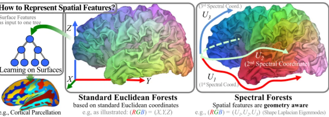
Standard Euclidean Forests
based on standard Euclidean coordinates e.g, as illustrated: (RGB) = (X,Y,Z)
Spectral Forests
Spatial features are geometry aware e.g., (RGB) = (U1,U2,U3) (Shape Laplacian Eigenmodes) Surface Features
as input to one tree
Learning on Surfaces
Z
X Y
How to Represent Spatial Features?
e.g., Cortical Parcellation
Fig. 1. Algorithm Overview– Whereas Standard Forests (RF) rely on spatial features
derived from Euclidean coordinates (x,y,z), Spectral Forests (SF) build geometry-aware
features using spectral coordinates (U1..k). This change of paradigm from extrinsic to
in-trinsicshape representation enables learning to be performed directly on surfaces. Coloring
indicates how spatial information is represented over the surface.
carry high expectations due to their promise in classifying various types of data in a fast manner. Unfortunately, their use in cortical analysis [14] has been limited due to the high geometrical variability of the folding pattern across individuals. Classi-fying cortical data on larger training sets may capture additional shape variability, however, one may wonder how to better exploit existing data, and how to capture maximal information on such complex surfaces. This raises the fundamental question on how to learn data directly on surfaces. We propose to use a different paradigm for representing spatial features in learning techniques.
Currently, a cortical point can be represented with pointwise data information, such as its depth on the cortex or its MRI pixel intensity. Feature representations are typically augmented with spatial information to uniquely characterize points in space, for instance, with its location in the Euclidean domain [15]. This, however, poses a problem since cortical surfaces highly vary in space and shape. Moreover, neighborhood structures, often exploited in image segmentation [16], may be am-biguous on surfaces, and more challenging to interpret on highly convoluted cortical surfaces. Neighboring positions in 3D space may in fact not necessarily lie on a sur-face, and be even several folds away on the cortex. Consequently, standard learning approaches that use features defined in the Euclidean domain, may not be adequate for cortical parcellation. We propose to represent instead spatial information with geometry-aware features. The spectral decomposition of shapes provides means to efficiently parameterize cortical surfaces with few spectral coordinates. More specif-ically, surface points are uniquely characterized with the eigenfunctions of an as-sociated graph Laplacian. Whereas its eigenvalues capture subject-wise properties, and can be used to identify subjects [17, 18], the eigenfunctions capture pointwise information directly on surfaces, and can be used, for instance, to match points be-tween cortical surfaces [19, 20]. Such named spectral coordinates constitute, in fact, an explicit parameterization of surfaces. A learning technique could thus exploit such spectral coordinates to learn data directly on surfaces. In this paper, we improve, for instance, the Random Decision Forests (RF) [21, 22], to process surface data via spectral representations of shapes, and name our method Spectral Forests (SF).
The next section details the fundamentals of Spectral Forests, followed by experi-ments evaluating the impact of using our spectral strategy over standard Euclidean approaches. We find a substantial improvement in accuracy in terms of Dice metric (from RF: 28%, to SF: 74%) and boundary distance error (RF/SF: 6.88/2.11mm).
2
Method
We begin by briefly reminding the fundamentals of Random Forests, and extend them for classifying data directly on surfaces.
Random Forests (RF) – A standard RF consists of an ensemble of decision trees, each making probabilistic decisions from input data, for instance, classifying cortical points into cortical parcels. During training, trees are grown by finding for each node, the binary test that best splits an input training data such that information gain among the class distributions is maximized. Each tree t learns a class predictor pt(c|f ) for a feature representation f , for instance, the sulcal depth and spatial coordinates
of a cortical point, fi = (depth(i), (x, y, z)i) at point i. During testing, unknown
points are classified by passing down their feature representations in ntreetrees. The
resulting class predictions are eventually averaged and a point is finally classified with
the maximal prediction ˆc = arg maxcPnT
i=1pti(c|f ). More details could be found in
[21, 22]. In standard RF, learning shape characteristics and locating their boundaries typically rely on spatial features that are derived from Euclidean coordinates, and neighborhoods are often implemented using random rectangles on a Cartesian grid [16]. Such features are not geometry aware, and rely on extrinsic shape information. Spectral Forests (SF) – We extend RF beyond the Euclidean domain, to classify surface data. To do so, spatial features are represented using spectral coordinates rather than Euclidean coordinates. They uniquely characterize surface points using the Laplacian eigenfunctions of a spectral shape decomposition [23]. These surface basis functions are geometry aware and have the property to be invariant to shape isometry. This is, for instance, exploited in cortical surface matching [19, 20], where, conveniently, corresponding points have similar spectral coordinates, even if they may not share the same location in space. Spectral representations effectively capture
intrinsic shape information. Location and neighborhoods are defined explicitly on
surfaces, which contrasts with the implicit representation of surfaces with Euclidean coordinates.
Spectral Coordinates – Let us build the graph G = {V , E } from the set of vertices with position x, and edges of a surface model S. We may define the |V | ×
|V | weighted adjacency matrix W in terms of node affinities, e.g., Wij =k xi −
xj k−1 if ∃eij ∈ E (inverse distance between neighboring points), 0 otherwise. The
diagonal node degree matrix D is the sum of all point affinities Di = PjWij.
The graph Laplacian operator is defined [24] as a |V | × |V | matrix L = D−1(D −
W ). Its spectral decomposition, L = U ΛU−1, provides the sorted eigenvalues Λ =
diag(λ0, ...λ|V |) and associated eigenfunctions U = (u(0), ..., u(|V |)), where u(·) is a
column of U and depicts in fact a vibration mode of shape S [25]. The spectral coordinates of points p ∈ V are defined as the eigenfunction values normalized by
their eigenvalues [23], spectral(p) = {λ−12
0 u(0)(p), ..., λ −1
2
|V |u(|V |)(p)}, which is a row
of matrix Λ−1
4
0
Standard Euclidean Forest Fails
(x,y,z) is too ambiguous as spatial information Best Case: Dice = 54.5% – dist = 4.92mm (±3.67, max 26.03)
Worst Case: Dice = 9.89% – dist = 9.77mm (±5.55, max 22.49)
Spectral Forest – Correct Segmentation
Spectral coordinates are geometry aware Best Case: Dice = 92.1% – Dist = 1.33mm (±1.22, max 7.45)
Worst Case: Dice = 82.0% – Dist = 1.94mm (±1.45, max 8.13)
Dice = 54.5% Dice = 92.1%
Red Contour: Ground Truth Black Contour: Forest Parcellation Inflated Surface
for Visualization
Calcarine Fissure
–80mm +80mm Color: Sulcal depth
Fig. 2. Segmentation of the Calcarine Fissure– which is deeply buried in a highly
convoluted area. (Left) Learning surface data with forests on standard Euclidean features produces low Dice scores, and a segmentation that is spatially inconsistent. (Right) Spectral Forests directly learn surface data via spatial features that are geometry aware. Surfaces are inflated only for visualization.
them would move us over the surface, whereas an increase in Euclidean coordinates may bring us away from the surface. For additional coherence, we further correct for slight perturbations in shape isometry, often observed as misalignment of spectral representations between subjects [26]. All representations are, therefore, realigned
to an arbitrary reference, Λ−1
2U Ti7→ref, where the transformation T is found, for
instance, with Iterative Closest Points (ICP) between spectral representations [26, 27]. In practice [19, 27], only the first k = 5 spectral coordinates are sufficient to capture the main geometrical properties. This keeps the computational expenses low, in the order of 2 seconds for a spectral decomposition and 1.5 seconds for an ICP refinement on a standard laptop computer. The spectral coordinates spectral(p)
for a point p of subject i, are therefore the first k elements of the pth row of matrix
Λ−1
2U Ti7→ref.
Cortical Parcellation – The labeling of cortical points into major sulci and gyri, is an application where learning should be performed on surfaces. Our Spectral Forests algorithm represents spatial information with spectral coordinates, which naturally parameterize surfaces in an intrinsic spectral domain rather than in an extrinsic Euclidean space, as shown in Fig. 1. The simplest form of feature representation
could be, for instance, fp = (depth(p), spectral(p)), which includes data
informa-tion, such as the sulcal depth at each point, and spatial informainforma-tion, where stan-dard (x, y, z) point values are replaced with k spectral coordinates. This change of paradigm enables a standard RF classifier to be applied on the spectral
representa-tion fp for learning and infering the major parcels over the brain surface.
3
Results
We now evaluate the performance of Spectral Forests (SF), with respect to standard Forests (RF) and FreeSurfer (FS), a leading software in cortical parcellation. Our dataset consists of 16 surfaces of white-grey matter interfaces generated from MRI, ranging from 109k to 174k vertices, each labeled into 77 cortical parcels obtained from a manual segmentation.
3.1 Euclidean versus Spectral Coordinates
The calcarine sulcus is of interest to studies in vision, however, its localization on the cortex remains difficult as it is deeply buried in a highly convoluted area of the visual cortex. Current methods, such as FS, typically involve a costly mesh deforma-tion toward a labeled atlas. Learning approaches could be an alternative, however, their use of spatial features derived from spatial coordinates may pose problems in representing location and neighborhoods. One could augment the representation of cortical points with extra information such as their sulcal depth on the cortex. This is the strategy adopted by FS.
Standard RF – To illustrate the benefits of using spectral coordinates over Eu-clidean coordinates, we choose to segment the calcarine sulcus in a binary classifica-tion, i.e., calcarine or not-calcarine. We first use standard RF with a simple feature
representation, fi = (depth(i), (x, y, z)i), with the sulcal depth of a point i and its
location in an Euclidean space. We use 50 trees, with 50k data points represented with the feature set f , and keep our parameters constant in all further experiments. We perform a leave-one-out evaluation, where 15 surfaces are used for each training, and test on the remaining surface. The average Dice overlap (2|A ∩ B|/(|A| + |B|)) for all 16 calcarine segmentations is 36.1% (± 10.5, min/max = 11.3/51.3). The average distance error between boundaries is on average 7.39mm (± 1.92, max (Hausdorff) 53.0). As seen on Fig. 2, the best case shows, in fact, mitigated results with an overlap of 51.3%, and boundary errors of 5.63mm (± 3.85, max 26.8). The consistent location of the predicted sulcus in deeper areas suggests that sulcal depth is a prominent feature during learning, however, spatial coherency of the resulting segmentation appears to be ambiguous. Despite a correct coarse positioning of the calcarine sulcus in the vision cortex, its precise location and delineation is imprecise. Euclidean features may not be adequate for learning on such convoluted surface. Indeed, two neighboring points in space, may not necessarily be close in term of geodesic distance on the surface, and may, in fact, even be several sulci apart. Spectral Forests – We now only modify the spatial features in order to fully
ap-preciate the impact of this fundamental change in Spectral Forests. We use fi =
(depth(i), spectral(i)), with sulcal depth and k = 5 spectral coordinates. With this simple change, surface data is now represented using geometry-aware features. The average overlap of the 16 calcarine segmentations is now improved to 89.4% (± 3.9%, min/max = 81.0/92.1), and the average boundary distance error is decreased to 1.56mm (± 0.39, max (Hausdorff) 11.25). This is a 147% improvement in over-lap, and 78% decrease in boundary error. A closer look on Fig. 2 shows indeed that this simple change of paradigm from Euclidean to spectral features produces a spa-tially coherent segmentation over the cortical surface. The computation time for RF and SF in this binary segmentation is 2.7 seconds for training, and 1.1 seconds for testing. Timing is measured on a 2.6GHz Core i7 with 16GB of RAM.
3.2 Full Cortical Parcellation
We now segment all 77 cortical parcels, and validate using the same leave-one-out approach with the same parameter set. Running standard RF produces an average overlap, for all 77 parcels on 16 surfaces, of 27.9% (± 17.0, min/max parcels = 4.9/65.9), and an average boundary error of 6.88mm (± 2.30, max (Hausdorff)
6
Parcellation – Standard Forest
Inconsistent Spatial Representation in Euclidean Space
Avg. Dice = 31.0%(±15.5) (One case, 77 parcels) Avg. Boundary Dist. = 5.80mm (±4.24, max 38.02)
Parcellation – Spectral Forest
Learning directly on a Surface Space
Avg. Dice = 77.6%(±11.41)
Avg. Dist = 2.02mm (±1.67, max 17.56)
FreeSurfer – Ground Truth
Variability of 16 parcellations (FreeSurfer)
Dataset Avg. Dice = 76.1%(±8.02)
Dataset Avg. Dist = 1.91mm (±1.57, max 13.01)
Fig. 3. Cortical Parcellation– (Left) Best cortical parcellation using RF (31.0%), which
reveals the limitation of using spatial features based on Euclidean coordinates, (Middle) Parcellation on same subject using SF (77.6%, our method), which shows an improved learning on cortical surfaces, (Right) using FS, considered here as gold standard. Inflated surfaces show 77 color-coded parcels. Central sulcus circled for visualization.
60.8). The required computation time is 21 seconds for training and 66 seconds for testing. Running Spectral Forests (SF) produces an average overlap of 74.3% (± 8.32, min/max parcels = 38.9/94.9), and a boundary error of 2.21mm (± 0.55, max (Hausdorff) 28.9). The computation time is 17 seconds for training and 23 seconds for testing. Fig. 3 shows the best scoring parcellation of RF, with an average overlap of 31.0% (± 15.5), which contrasts with the SF parcellation on the same subject of 77.6% (± 11.41). One can observe the improvement in spatial consistency of the surface segmentation between RF and SF, where, for instance, the central sulcus (circled in yellow) is barely distinguishable using RF. In comparison, FreeSurfer (FS), which is considered here as a gold standard, performs with an average overlap of 74.4% (± 9.7, min/max parcels = 41.2/96.6) among all possible transfers of parcellation maps from all subjects onto all possible reference subjects. The average boundary distance error between all possible transfers of cortical maps is 2.21mm (± 0.75, max (Hausdorff) 37.5). This evaluates the variability of FS in mapping cortical parcellations. The performances of SF (74.3%, 2.21mm) and FS (74.4%, 2.21mm) are arguably similar, however SF have a clear speed advantage over FreeSurfer. Full cortical parcellation in SF takes on average 23 seconds at test time, whereas FS requires 3 to 4 hours of computation due to its slow mesh inflation process. We also observed that trees have roughly 9k nodes with SF, and 23k nodes with RF. This may explain the computational advantage of SF over RF (17+23secs over 21+66secs, for training+testing time), and perhaps indicate that information may be better structured with spectral features, producing less tree nodes than with Euclidean features. Fig. 4 summarizes the overlap and boundary errors for all 77 parcels in our leave-one-out validation. It is interesting to observe that with the unique change of spatial features, from Euclidean to spectral coordinates, the average parcel overlap is consistently higher in SF than RF (74.3% vs. 27.9%). Similarly, the boundary error is consistently lower in SF than RF (2.21mm vs. 6.88mm). In addition, SF shows equivalent performance than the state-of-the-art (FreeSurfer in green) but at a significant fraction of its costs (23 seconds for SF vs. 3 to 4 hours for FS).
Dice Scores for 77 parcels
Standard Forest (Avg.: 27.9%) Spectral Forest (Avg.: 74.3%)
Boundary Distance Errors for 77 parcels
Standard Forest (Avg.: 6.88mm) Spectral Forest (Avg.: 2.21mm) 0% 50% 100% 0mm 6mm 120mm 1 10 20 30 40 50 60 70 1 10 20 30 40 50 60 70 Parcel IDs Parcel IDs
Spectral Forests give higher Dice Scores
Spectral Forests give lower Distance Errors
D is tanc e E rr or (m m ) A cc ur ac y (%) FreeSurfer (Avg.: 2.21mm) FreeSurfer (Avg.: 74.4%)
Fig. 4. Evaluation per parcel– (Top) Dice Metric and (Bottom) Boundary Distance
Error for all 77 cortical parcels, using RF (Red ), SF (Blue, our method), and FS (Green curve, given for comparison). SF provide consistently higher Dice scores than RF (74.3% vs. 27.9%), and has an equivalent accuracy than FS, but only at a fraction of its cost (23 seconds vs. 3 to 4 hours for FS).
4
Conclusion
In this paper, we tackled the difficult problem of learning data on complex sur-faces, such as the cerebral cortex. Whereas conventional approaches would represent spatial information with extrinsic, or implicit, representations, we proposed to use geometry-aware features that are based on the spectral decomposition of shapes. This change of paradigm from extrinsic to intrinsic shape representations, or from
implicit to explicit surface parameterization, enables learning techniques to process
data directly on surfaces. We implemented this new strategy using the Random De-cision Forests model, and named our method Spectral Forests. We illustrated its impact with an application to cortical parcellation, which involves complex surfaces with highly varying folding patterns across individuals. We found that revisiting the fundamentals of spatial representations, from Euclidean to spectral-based features, improves the parcellation accuracy from 27.9% to 74.3%, which is comparable to the present state-of-the-art, but with a clear speed advantage (23 seconds vs. hours). Our experiments showed that simple spatial representations with pure spectral coordi-nates, on a relatively small dataset, can already track the accuracy of FreeSurfer. We may possibly expect further improvements with more advanced spectral features, for instance, by exploiting neighborhoods on surfaces. Nonetheless, our approach high-lights the pertinence of using geometry-aware features in learning techniques. The use of Spectral Forests may also be relevant beyond the analysis of cortices, for in-stance, in studying surfaces of other organs, or more generally, in applications where data lives on surfaces.
Acknowledgment – This research is partially funded by the ERC Advanced Grant MedYMA and the Research Council of Canada (NSERC).
8
References
1. Behnke, K.J., Rettmann, M.E., Pham, D.L., Shen, D., Resnick, S.M., Davatzikos, C., Prince, J.L.: Automatic classification of sulcal regions of the human brain cortex using pattern recognition. TMI (2003)
2. Li, G., Shen, D.: Consistent sulcal parcellation of longitudinal cortical surfaces. Neu-roImage (2011)
3. Le Goualher, G., Procyk, E., Collins, D.L., Venugopal, R., Barillot, C., Evans, A.C.: Automated extraction and variability analysis of sulcal neuroanatomy. TMI (1999) 4. Lohmann, G., von Cramon, D.Y.: Automatic labelling of the human cortical surface
using sulcal basins. Med. Image Anal. (2000)
5. Rivi`ere, D., Mangin, J.F., Papadopoulos-Orfanos, D., Martinez, J.M., Frouin, V., R´egis, J.: Automatic recognition of cortical sulci of the human brain using a congregation of neural networks. Med. Image Anal. (2002)
6. Fischl, B., Sereno, M.I., Tootell, R.B., Dale, A.M.: High-resolution intersubject aver-aging and a coordinate system for cortical surface. HBM (1999)
7. Fischl, B., van der Kouwe, A., Destrieux, C., Halgren, E., Segonne, F., Salat, D.H., Busa, E., Seidman, L.J., Goldstein, J., Kennedy, D., Caviness, V., Makris, N., Rosen, B., Dale, A.M.: Automatically parcellating the human cerebral cortex. Cereb. Cortex (2004)
8. Rettmann, M.E., Han, X., Xu, C., Prince, J.L.: Automated sulcal segmentation using watersheds on the cortical surface. NeuroImage (2002)
9. Yang, F., Kruggel, F.: Automatic segmentation of human brain sulci. Med. Image Anal. (2008) 10. Li, G., Guo, L., Nie, J., Liu, T.: Automatic cortical sulcal parcellation based on surface
principal direction flow field tracking. NeuroImage (2009)
11. Shi, Y., Tu, Z., Reiss, A.L., Dutton, R.A., Lee, A.D., Galaburda, A.M., Dinov, I., Thompson, P.M., Toga, A.W.: Joint sulcal detection on cortical surfaces with graphical models and boosted priors. TMI (2009) 361–73
12. Shattuck, D.W., Joshi, A.A., Pantazis, D., Kan, E., Dutton, R.A., Sowell, E.R., Thomp-son, P.M., Toga, A.W., Leahy, R.M.: Semi-automated method for delineation of land-marks on models of the cerebral cortex. Neuroscience (2009)
13. Cachia, A., Mangin, J.F., Rivi`ere, D., Papadopoulos-Orfanos, D., Kherif, F., Bloch, I., R´egis, J.: A generic framework for the parcellation of the cortical surface into gyri using geodesic Vorono¨ı diagrams. Med. Image Anal. (2003)
14. Tu, Z., Zheng, S., Yuille, A.L., Reiss, A.L., Dutton, R.A., Lee, A.D., Galaburda, A.M., Dinov, I., Thompson, P.M., Toga, A.W.: Automated extraction of the cortical sulci based on a supervised learning approach. TMI (2007)
15. Stough, J.V., Ye, C., Ying, S.H., Prince, J.L.: Thalamic Parcellation from Multi-modal Data using Random Forests. ISBI (2013)
16. Lempitsky, V., Verhoek, M., Noble, Blake, A.: Random forest classification for auto-matic delineation of myocardium in real-time 3D echocardiography. In: FIMH. (2009) 17. Konukoglu, E., Glocker, B., Criminisi, A., Pohl, K.: WESD - Weighted Spectral
Dis-tance for Measuring Shape Dissimilarity. PAMI (2012)
18. Wachinger, C., Golland, P., Kremen, W., Fischl, B., Reuter, M.: BrainPrint: A Dis-criminative Characterization of Brain Morphology. NeuroImage (2015)
19. Lombaert, H., Grady, L., Polimeni, J., Cheriet, F.: FOCUSR: Feature Oriented Corre-spondence using Spectral Regularization - A Method for Accurate Surface Matching. PAMI (2012)
20. Shi, Y., Lai, R., Wang, D.J.J., Pelletier, D., Mohr, D., Sicotte, N., Toga, A.W.: Metric optimization for surface analysis in the Laplace-Beltrami embedding space. TMI (2014) 21. Breiman, L.: Random forests. Mach. Learn. 45 (2001)
22. Criminisi, A., Shotton, J.: Decision Forests for Computer Vision and Medical Image Analysis. Springer (2013)
23. Rustamov, R.M.: Laplace-Beltrami eigenfunctions for deformation invariant shape rep-resentation. In: Eurographics. (2007)
24. Grady, L., Polimeni, J.R.: Discrete Calculus. Springer (2010) 25. Chung, F.: Spectral Graph Theory. AMS (1996)
26. Mateus, D., Horaud, R., Knossow, D., Cuzzolin, F., Boyer, E.: Articulated shape match-ing usmatch-ing Laplacian eigenfunctions and unsupervised point registration. In: CVPR. (2008)
27. Lombaert, H., Arcaro, M., Ayache, N.: Brain Transfer: Spectral Analysis of Cortical Surfaces and Functional Maps. In: IPMI. (2015)