Drift-driven cross-field transport and Scrape-Off Layer width in the limit of low anomalous transport

HAL Id: hal-01671477

https://hal.archives-ouvertes.fr/hal-01671477

Preprint submitted on 22 Dec 2017

HAL is a multi-disciplinary open access

archive for the deposit and dissemination of

sci-entific research documents, whether they are

pub-lished or not. The documents may come from

teaching and research institutions in France or

abroad, or from public or private research centers.

L’archive ouverte pluridisciplinaire HAL, est

destinée au dépôt et à la diffusion de documents

scientifiques de niveau recherche, publiés ou non,

émanant des établissements d’enseignement et de

recherche français ou étrangers, des laboratoires

publics ou privés.

Drift-driven cross-field transport and Scrape-Off Layer

width in the limit of low anomalous transport

Camille Baudoin, Patrick Tamain, Hugo Bufferand, Guido Ciraolo, Nicolas

Fedorczak, Davide Galassi, Alberto Gallo, Philippe Ghendrih, Nicolas Nace

To cite this version:

Camille Baudoin, Patrick Tamain, Hugo Bufferand, Guido Ciraolo, Nicolas Fedorczak, et al..

Drift-driven cross-field transport and Scrape-Off Layer width in the limit of low anomalous transport. 2017.

�hal-01671477�

Drift-driven cross-field transport and Scrape-Off Layer width in the limit of low

anomalous transport

Camille Baudoin

_{, Patrick Tamain}

_{, Hugo Bufferand}

_{, Guido Ciraolo}

_{, Nicolas Fedorczak}

_{, Davide Galassi}

_,

Alberto Gallo

_{, Philippe Ghendrih}

_{, and Nicolas Nace}

1

_{CEA, IRFM, F-13108 Saint-Paul-lez-Durance, France}

2

_{Aix Marseille Univ, CNRS, Centrale Marseille, M2P2, Marseille, France}

21 d´

ecembre 2017

Abstract

The impact of the ∇B-drift in the cross-field transport and its effect on the density and power scrape-off layer (SOL) width in the limit of low anomalous transport is studied with the fluid code SolEdge2D. In a first part of the work, the simulations are run with an isothermal reduced fluid model. It is found that a ∇B-drift dominated regime is reached in all geometries studied (JET-like, ASDEX-like and circular analytic geometries), and that the transition toward this regime comes along with the apparition of supersonic shocks, and a complex parallel equilibrium. The parametric dependencies of the SOL width in this regime are investigated, and the temperature and the poloidal magnetic field are found to be the principal parameters governing the evolution of the SOL width. In the second part of this paper, the impact of additional physics is studied (inclusion of the centrifugal drift, self-consistent variation of temperature and the treatment of the neutral species). The addition of centrifugal drift and neutral species are shown to play a role in the establishment of the parallel equilibrium, impacting the SOL’s width. Finally, the numerical results are compared with the estimate of the Goldston’s heuristic drift based model (HD-model), which has showed good agreement with experimental scaling laws. We find that the particles SOL’s widths in the ∇B-drift dominated regime are, at least, two times smaller than the estimate of the HD-model. Moreover, in the parametric dependencies proposed by the HD-model, only the dependency with Bpol

is retrieved but not the one on T .

1

Introduction

Economical viability of future fusion devices requires a sufficient power spreading on Plasma Facing Component (PFC) poten-tially damaged by high energy deposition, for ITER the divertor materials constraint in steady state is estimated at 10 MW/m2

[1]. For a given PSOL, qmax is set by SOL heat channel width, commonly named λq, and divertor spreading Sq [2], hence the heat

channel width is a key parameter for tokamak operation.

The description of heat load at the target [2] which takes into account both transport in the main Scrape-Off Layer (SOL) and the in the divertor region, has permitted to get rid of the geometrical effects and to extract a coherent multi-machine (JET, DIII-D, ASDEX-Upgrade, C-Mod, NSTX, MAST) empirical scaling law for H-mode [3, 4]. The strongest dependency found is the one with Bpol, giving λq,Eich∝ Bpol−1.16. This functional dependencies has been retrieved in other experiments, in MAST [5] and in

λTe at the mid-plane, in agreement with Eich’s scaling considering a two point model [6]. It is worth to note that this feature is not specific to H-mode, an empirical scaling law on JET and ASDEX-Upgrade in L-mode shows similar dependency with Bpol [7, 8].

The extrapolation of the H-mode scaling law to ITER has predicted λq= 1 mm raising concern for future reactor device.

So far, empirical scaling laws miss a theoretical ground to confirm their prediction, and the mechanisms driving the heat transverse transport in the edge plasma are not yet fully understood. This is a central issue for the design and the sizing of future devices. Some theoretical studies attempt to describe the way energy escapes the core plasma through the separatrix and deposits on the PFC have been done, but no definitive conclusion have been drawn yet. In L-mode, it is accepted that turbulence dominates the cross-field transport, theoretical model have been proposed based on linear analysis using the gradient removal theory [9], and based on a blob approach [10] to predict the value of the SOL width in L-mode. In H-mode turbulence is strongly reduced in the pedestal and near-SOL. It is thus not clear which is the main mechanism driving the transport through the separatrix. A Heuristic Drift-based (HD) model [11] proposed that the curvature drift is the main mechanism driving the cross-field transport across the separatrix in H-mode determining entirely the SOL power width. Similar description of the edge transport were earlier proposed by

Ref. [12] with a neoclassical approach. This model has attracted much interest for its good agreement with experience [3, 13, 14], in particular its prediction of the dependency on Bpol.

The work presented in this paper aims at understanding the convective transport via the curvature drifts, in the limit of weak collisional and anomalous transport. Similar work has been published [15, 16] assessing the existence of a regime where the SOL width is determined by ∇B-drift. In this study, we use a different numerical model, the 2D fluid code SolEdge2D, to further investigate the framework of such a ∇B-drift dominated regime : its characteristic, its dependencies on parameters and on geometry, and its limits. In particular, we study the impact of the addition of the centrifugal drift, the inclusion of temperature variation and of the neutral species.

We first seek for a regime where the level of turbulence, set via a diffusion coefficient in the model, does not impact the SOL width. Even in a low turbulence regime, it is not obvious that the magnetic drift could contribute significantly to the flux-surface averaged transport as the drift presents an up/down symmetry. Hence, an outward flux-surface transport would require a strong up/down asymmetry [17]. We then characterize such a regime and finally compare the SOL width to the estimate of the heuristic model.

After a brief description of the SolEdge2D model (section 2), the impact of the ∇B-drift on cross-field transport, plasma parallel equilibriums and radial profiles is first studied at different levels of anomalous transport in a JET-like geometry (section 3). After establishing the existence of a ∇B-drift dominated regime, we estimate SOL widths found in such a regime. We also look at the parametric functional dependencies (section 3.4) and the impact of geometry on the SOL width (section 4). In section 5, we study the impact of the centrifugal drift, another component of the magnetic drift not always taken into account in fluid models. In section 6, we release the isothermal assumption and we study the impact of the inclusion of neutral species. Finally, in section 7, we draw a comparison between of numerical results and the estimate of the HD-model for the SOL width, and we discuss the assumptions made in the model.

2

Model description : setup and geometry

In this section, the model used for this study is briefly described, see [18] for more details. SolEdge2D is a mean-field transport code that assumes toroidal axisymmetry of all field and solves Braginskii equations for electrons and an arbitrary number of ions species. In the single ion case, of interest in this paper, the model solves for the ion density n, parallel ion velocity u∥, and temperature of electrons and ions Teand Ti (1)-(4) which are solved using a finite volume numerical scheme. At the scale of the

mesh grid, larger than the Debye length, the quasi-neutrality is justified give n= ne= ni. Moreover, in this work, we don’t consider

the physics of charge balance, thus we assume u_∥ = u_∥,e = u_∥,i. This is an important assumption since the ∇B-drift is charged dependent and induces a plasma polarisation which should be discussed.

∂tn+ ∇ ⋅ (nu∥b+ nu⊥) = Sn (1) ∂t(nu∥) + ∇ ⋅ (nu∥(u∥b+ u⊥)) = −∇∥ pi mi+ qinE∥ mi + Rei mi + ∇ ⋅ (ν ⊥n∇⊥u_∥) + Snu (2) ∂t( 3 2nTi+ 1 2minu 2 ∥) + ∇ ⋅ (( 5 2nTi+ 1 2minu 2 ∥) (u∥b+ u_⊥)) = ∇ ⋅ (κi∇_∥Tib+ χ⊥n∇⊥Ti+ ν⊥n∇⊥( 1 2miu 2 ∥)) + qinu∥E∥+ u∥Rei+ Qei+ SEi (3) ∂t( 3 2nTe) + ∇ ⋅ ( 5 2nTe(u∥b+ u⊥)) = ∇ ⋅ (κe∇∥Teb+ χ⊥n∇⊥Te) − enu∥E∥− u∥Rei− Qei+ S Ee ₍₄₎

Where b denotes the direction of the magnetic field b= B_B, and Qei is an energy transfer due to collision. The inertia and viscosity

terms of electrons are neglected giving enE_∥= ∇_∥(pe)−Reiwhere E∥is the parallel electric field and Reiis the parallel friction force.

In standard 2D transport code, turbulence is inhibited as turbulence requires the treatment of the two transverse directions and the cross-field anomalous transport is arbitrarily set via diffusion operator. The cross-field flux is then equal to nu_⊥= −D_⊥∇_⊥n+nu_drift.

The diffusion coefficient D_⊥ stands for the local level of anomalous transverse transport. For all the following simulations, D_⊥ is set to 1 m2_s−1 _{on a zone of few millimeters at the inner and outer borders to avoid edge effect, and is a constant, labeled D, on}

the rest of the grid. D is the main free parameter of this work and will be scanned to study the impact of the fluid drifts on the transverse transport for different levels of anomalous transport. The viscosity ν is equal to the diffusivity D, and ion and electron thermal diffusivities are fixed to 1 m2_s−1_{on the all domain. In this work, only the magnetic drift are considered, u}

drift= u∇B,i+uc,

where u_∇B (5) denotes the ∇B-drift (in the fluid approach nu_∇Bdivergence coincides with the divergence of the diamagnetic drift flux), and ucent(6) denotes the centrifugal drift [19].

u∇B,i= B× ∇pi

(a) JET

2.0 2.5 3.0 3.5

R

(m)

1

0

1

2

Z

(m

)

0.3

0.5

0.7

R

(m)

0.3

0.0

0.3

Z

(m

)

0.8

1.0

1.2

R

(m)

0.2

0.0

0.2

Z

(m

)

Figure 1 – Sketch of computational grid (black lines) for the diverted JET-like (a) and COMPASS-like (b) plasma equilibria with the wall position (red lines), (c) for the analytical circular equilibrium with the limiter position (red lines) ; for the purpose of legibility only one in three edges in reported for JET-like grid and one in four for circular geometry

ucent=

mv2 ∥

qB2B× b ⋅ ∇b (6)

The magnetic field is in the normal direction, that is to say u_∇B is downward for ions. The study of electrical drift is out of the scope of this work and a reduced model of SolEdge2D is considered where the electric drift is omitted. Three set of simulations are considered : 1) simulations including no drifts, referred as diffusion simulations, 2) simulations with including only ∇B-drift, and 3) simulations including both ∇B and centrifugal drifts. In a first stage, section 3 - 5, the plasma is supposed isothermal, and T is constant on all the domain, with Te= Ti= 50 eV, and neutrals are not taken into account. These assumptions are relaxed in

section 6 to evaluate how they impact the transport and plasma equilibriums.

The simulated domain extends from closed flux surfaces in the vicinity of the separatrix, with Dirichlet condition imposed to density n= 10−19m−3at the core boundary, to open flux surfaces up to the wall. In the parallel direction Bohm boundary condition are imposed at the sheath entrance. Simulations have been run for three magnetic equilibrium, as illustrated on Fig 1, a) a realistic diverted JET-like geometry on a 80× 139 (r, θ)-grid with the following parameters R0 = 2.895 m, a = 0.950 m, the safety factor

q95, defined as the safety factor on the flux-surface ψ such as ψ/ψsep = 0.95, is about 5 in the near SOL and B0 = 2.2 T, b) a

realistic diverted COMPASS-like geometry on a 48× 139 (r, θ)-grid with the following parameters R0= 0.55 m, a = 0.17 m, q95≈ 4,

B0= 1.15 T, 2) an analytical circular geometry on a 240 × 180 (r, θ)-grid, with the following parameters R0= 1.075 m, a = 0.287 m,

q95 ≈ 4, B0= 1 T. On diverted equilibrium, a penalization technique is used that enable simulation of the plasma up to the first

wall reported with a red line on Fig 1 a and b.

3

Convective transport by u

at low anomalous transport in JET-like geometry

3.1

∇

B-drift dominated regime in the limit of low anomalous transport

To study the role played by the ∇B-drift in the particle transverse transport, two sets of JET-like isothermal simulations are first considered, the diffusive case, and the case including only the ∇B-drift, for various levels of D. In these sets of simulations the coefficient D is scanned between 1 m2s−1and 2.0× 10−4m2s−1, with the aim to find out whether a regime where the large-scale convection by u_∇B is the main mechanism of particle transverse transport exists and what would be the properties of such plasma equilibrium.

On Fig. 2a) total particle flux through the separatrix due to diffusion process (7) and to the convection via u_∇B(8) are reported for both ∇B-drift and purely diffusive simulations as a function of D. Note that all fluxes are normalized by the mean density at the separatrix.

(a)

10

₁₀

₁₀

₁₀

₁₀

D

(m

_.

s

)

10

10

10

10

Γ

/n

Dth

Γ

Γ

Γ

0.0 0.2 0.4 0.6 0.8 1.0

Normalized poloidal distance from LFS divertor entrance

0.5

0.0

0.5

1e20

Γ

Γ

Γ

0.0 0.2 0.4 0.6 0.8 1.0

Normalized poloidal distance from LFS divertor entrance

2

0

2

1e19

Γ

Γ

Γ

Figure 2 – (a) : Total particle fluxes through the separatrix normalized by the mean density due to diffusion process (blue square), to centrifugal drift (red square) for ∇B-drift simulations, and for diffusive simulations (black triangles) as a function of D. (b), (c) : Poloidal distribution of the particle flux : global (full line), by diffusion (dot-dashed line), by u_∇B (dashed line) for D= 1 × 10−1m2s−1 (b) and D= 1 × 10−3m2s−1(c) Γ_⊥,D= ∫ sep−D⊥ ∇_⊥n⋅ ∇ψ (7) Γ⊥,∇B= ∫ sepnu∇B⋅ ∇ψ (8)

For D≥ 1 × 10−2m2_s−1_{, the diffusive operator is responsible of all the transport and the averaged convective u}

∇B flux is even sightly negative. In that range of D, there is no significant difference of Γ_⊥,nbetween simulations with or without drift, in both cases the particle flux scales as√D, expected for a standard diffusive process. At D=1 × 10−2m2s−1, the u_∇B convective contribution in the particles balance starts to rise and its relative weight continues to rise with the decreasing level of transverse transport to end up largely dominant for D≤ 1 × 10−3m2s−1, with a contribution of more than 90% in the total balance. Hence a ∇B-drift dominated regime is reached at low transverse transport. In the following of the paper, we denote Dth we value of D at the transition toward

the ∇B dominated regime. At this level of D, the diffusion source in the ∇B-drift simulations decreases faster than for the purely diffusive simulations due to a relative flattening of the radial profile around the separatrix (see section 3.3).

To give an indication of what would represent such a level of transverse transport, let us recall some typical value of the diffusion coefficients used when addressing anomalous transverse transport, as well as classical and neoclassical processes. The typical diffusion for anomalous transport used in the pedestal to match profiles in H-mode plasmas is of the order of 1× 10−1m2_s−1

[20, 21, 22, 23] the estimation of diffusion representing the dissipative process as established in [24] give a typical diffusion of DC≈ 1.5 × 10−3m2s−1for classical processes and DNC≈ 2.5 × 10−2m2s−1for neoclassical process. Thus the transition toward a drift

dominated regime appears to take place well below the neoclassical level and u_∇B is predominant only at a diffusion level lower than the classical level, which raises the question of the possibility of achieving such a regime.

It is important to stress that the appearance of a flux-surface averaged particle transport by u_∇B is inevitably associated with strong poloidal asymmetries. Indeed Γ_∇B = ∫_sepnu_∇B⋅ ∇ψ yet ∫_sepu_∇B⋅ ∇ψ = 0 due to the vertical symmetry of the ∇B-drift implying that a sufficient up/down asymmetry is necessary to permit Γ∇Bto be positive. On Fig. 2b. and 2c. the poloidal local flux is reported, at relatively high diffusion D= 0.1 m2_s−1_{, u}

∇B convection is then found to contribute significantly locally, but with the symmetry the positive flux at the bottom strictly compensates the sink at the top, so the flux-surface contribution is negligible. At low anomalous transport, Fig. 2c, the u_∇B convective flux exhibits an up-down asymmetry, and the source at the bottom of the torus becomes bigger than the sink at the top, explaining the rise of its weight in the flux-surface balance.

3.2

Equilibrium in drift dominated regime

In the previous section, it has been shown that at D (D≤ 1 × 10−3m2s−1) the convection by u∇B is the predominant particle source for the SOL, at both local and global scales. Let us now characterise the plasma equilibrium in such a regime. On Fig. 3, the poloidal profiles in the near SOL of density (a) and Mach number M=

√_m

iu∥

√

Te+Ti (b) are reported. At D> 2 × 10

−2 _{density is almost}

constant in the poloidal direction, and the Mach number relatively low far from the target. At low D, the most striking result is the appearance of a complex parallel equilibrium presenting a supersonic transition that comes along with the rise of sharp gradients and strong asymmetry of the density in the poloidal direction. Note that the density tends to be higher at the bottom of the torus, in agreement with the direction of the u∇B convection which leads to an effective particle source. This supersonic transition at

(a)

0.0

0.2

0.4

0.6

0.8

1.0

Normalized poloidal distance from LFS divertor target

0.4

0.6

0.8

1.0

N

/N

0.0

0.2

0.4

0.6

0.8

1.0

Normalized poloidal distance from LFS divertor target

1

0

1

Mach number

Figure 3 – Poloidal profile in the near SOL (ar= 1.004) of the normalized density (a), and the parallel Mach number (b) for ∇B-drift

simulations for D = 1 × 10−1m2_s−1 _{(red line with square), D = 5 × 10}−3_m2_s−1 _{(blue line with triangles), and D= 2 × 10}−4_m2_s−1

(black line with circle)

low D comes from the strong asymmetry of the effective particle source, composed of a large source at the bottom of the torus and a large sink at the top, creating important Pfirsch–Schl¨uter return flow. When decreasing the diffusion coefficient, the pressure gradient increases, and it enlarges the Pfirsch–Schl¨uter flows amplitude (Γ_{∥,P S} ∝ ∇P), reaching a supersonic transition coming along with a steady-state shock in the poloidal direction. It has been verified that the transition is in agreement with the model of supersonic transition presented in [25] with the annulation of derivative the parameter control A= _1+M2M2 at each transition between subsonic and supersonic flows.

In fact this transition can be explained by a reduced model for the parallel equilibrium Eq. (9). In a steady-state equilibrium, the continuity equation and the momentum balance can be simplified in Eq. (9) by assuming that : 1) the parallel particle flux distribution is of the form S1+ S2cos(

2πz∥

L∥ ), where z∥

is the parallel coordinate and L_∥the parallel length, representing a constant diffusive flux and a sinusoidal u_∇Bflux in a circular geometry, 2) the total pressure is uniform in the parallel direction (i.e nT(1+M2₎

is conserved), 3) the Mach number is equal to 1 at both targets. ⎧⎪⎪⎪ ⎪⎪⎪ ⎨⎪⎪⎪ ⎪⎪⎪⎩ ∂z∥Γ∥= S1+ S2cos( 2πz∥ L∥ ) ∂z∥( Γ2 ∥ n + n) = 0 with Γ∥= nu∥ ∣M∣ = 1 for z∥= 0, L∥ (9)

This system has the following analytical solution : ⎧⎪⎪⎪ ⎪⎪ ⎨⎪⎪⎪ ⎪⎪⎩ Γ_∥(z_∥) = S1(z∥− 0.5) + S2sin( 2πz∥ L∥ ) M(z_∥) =1₂(−1 ±√∆) with∶ ∆ = S2 1− 4Γ∥(z∥) 2 (10)

It is found that for S2

S1 > 4.6 no subsonic smooth solution exists, thus it allows us to predict the threshold in D when the supersonic bifurcation first appears. Let us now estimate the value of diffusion where the supersonic transition should occur. The diffusive particle flux is equal to D∇_⊥n = D_λn

n, with λn =

√_2πqR 0D

cs for a standard diffusive process. For the contribution of the ∇B-drift, the coefficient S2 correspond to the maximum of the flux by diamagnetic drift S2 = nu∇B,max, note that u∇B in

the isothermal case in only a function of the geometry as the temperature is imposed. Thus the bifurcation toward a supersonic transition should appear when u∇B

D λn =

√

2πqR√ 0u∇B

csD = 4.6. The numerical application gives Dtrans ≈ 1.5 × 10

−2_m2_s−1 _{for a JET-like}

configuration. In simulations supersonic flows first occur at D= 5 × 10−3m2_s−1 _{that it to say at lower diffusion than predicted.}

This discrepancy can be explained by the assumption of a circular geometry in our model Eq. (9). Moreover, the numerical scheme order was shown to impact the value of the transition through its ability or not to capture shocks accurately. In fact for a circular geometry with a 2nd order WENO scheme the model predict the correct value of Dtrans. It is worth to note that the rise of the

u_∇B convective transport appears at the same diffusion than supersonic transition, therefore it seems to be a necessary condition to be in a drift dominated regime of transport as it allows strong symmetry breaking of the density.

(a)

-5

0

5

d

(mm)

10

10

10

10

N

/N

20

0

20

40

d

(mm)

0.0

0.5

1.0

N

/N

Figure 4 – Density radial profile for diffusive (dashed lines) and ∇B-drift (full lines) simulations at the outer mid-plane (a), and at the outer target (b), for D= 1 × 10−1m2_s−1 _{(red), and D= 2 × 10}−4_m2_s−1 _(black)

0.0 0.1 0.2 0.3 0.4 0.5

Normalized poloidal distance from LFS divertor entrance 0.0 0.5 1.0 1.5 2.0 λint (mm) LFS mp TOP

Figure 5 – Poloidal profile of λn,int for diffusive (dashed line), ∇B-drift (full line) and both ∇B and centrifugal drift (dot-dashed

line) simulations for D= 2 × 10−4m2s−1

10

₁₀

₁₀

₁₀

₁₀

D

(m

_.

s

)

10

10

λ

(m

m

)

λ

Figure 6 – λn,Eich for purely diffusive (black triangles), and for ∇B-drift (red square) simulations as a function of the diffusion

coefficient, the dashed straight lines represents the √D scaling, and the x- and y-axis are in log-scale, for JET-like simulation

3.3

SOL width and scaling

We now aim to define a SOL width looking at the radial profiles Fig. 4 at the outer mid-plane (a) and at the outer target (b). For D < Dth radial profiles follow the classical description of a decreasing exponential. Profiles of both set of simulations,

with or without u∇B, coincide except for a small inward shift of the peak at the outer target due to the inward direction of u_∇B below the X-point. However for simulations with supersonic transitions, profiles of simulations with and without drift differ significantly. Moreover, profiles at the outer mid-plane of ∇B-drift simulation are not well fitted by an exponential function, thus the definition of SOL width by a single e-folding length is no longer relevant. Hence, we use the so-called integral decay length defined by λint= ∫ n(r)dr/nmax. This is a convenient definition as it permits to compare exponential profiles with more complex

ones, furthermore it is meaningful as it is directly linked to the peak value. Another way to define the SOL’s width, most commonly used in experiments [3], is to proceed with an Eich’s fit [2], convolution of a decreasing exponential and a Gaussian at the outer target profile, the resulting estimation of the SOL width is denoted λn,Eich. Since it is the most commonly used in experiments, the

Eich’s definition is prioritized. Nevertheless, if in this set of simulations profiles at the outer target are well described by an Eich’s fit, it is not always the case, and in such cases we settle for the integral description. Note that all estimates of SOL width take into account the flux expansion by remapping profiles at the outer mid-plane in order to get rid of obvious geometric effects.

It is also important to point out that gradients vary not only in the radial direction but also in the poloidal direction. On Fig 5 we observe that at low diffusion λn,intis uniform for purely diffusive simulations, but presents variation in the poloidal direction in

the drift dominated regime. Note that here variations are moderate but in other set of simulations (see section 5) poloidal variation amplitude of λn,intcan reach a factor 4. In conclusion, one must keep in mind that an estimation of a SOL width by a single value

summarises the transverse transport but is an oversimplification and hides the complexity of the plasma equilibrium.

On Fig. 6, λn,Eichis reported as a function of D. The estimate of the HD-model λHDfor the simulation parameters and geometry is

also reported in blue dashed lines, the comparison with the model will be discussed in the last section of this paper. We observe a perfect√D scaling for purely diffusive simulations. The code is therefore robust in this low diffusion regime and is not dominated

(a)

40

60

80

100

T

(eV)

0.8

1.0

1.2

1.4

λ

(m

m

)

0.8

1.0

1.2

1.4

α

0.6

0.8

1.0

1.2

1.4

1.6

λ

(m

m

)

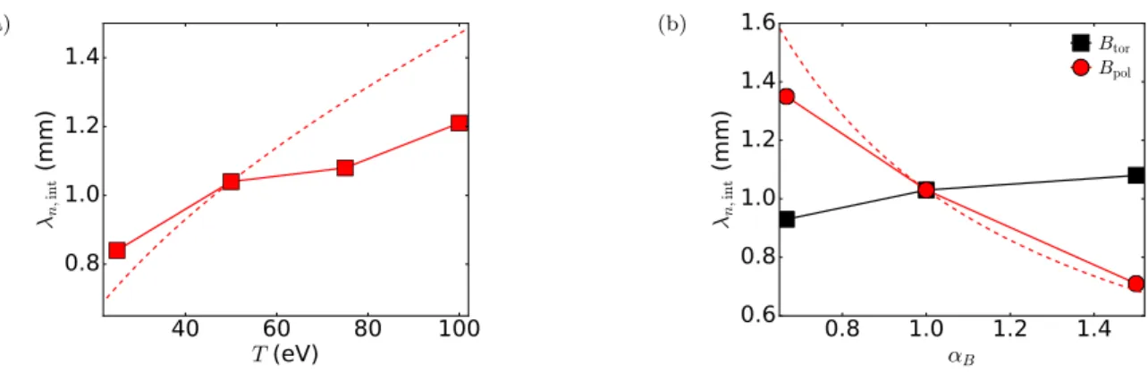
Figure 7 – λn,int SOL for ∇B-drift simulations at D = 2 × 10−4m2s−1 as a function of the temperature with red dashed lines

representing the√T scaling (a) and as a function of the multiplicative factor, αB, on Bpol and Btor with dashed lines representing

the B_pol−1 scaling (a)

0.0 0.1 0.2

Normalized poloidal distance from LFS divertor

1 0 1 Mach number % T LFS mp mp LFS X-pt (b) 0.0 0.1 0.2

Normalized poloidal distance from LFS divertor

1 0 1 Mach number & Bpol LFS mp mp LFS X-pt

Figure 8 – Mach number poloidal profile in the near SOL, for ∇B-drift simulations for D= 2 × 10−4m2s−1for several temperature T = 25 eV, 50 eV, 75 eV and 100 eV respectively blue, green, red, cyan lines, and different Bpol = 1/1.5, 1, 1.5 × Bpol,0 respectively

blue, green, red lines

by spurious numerical diffusion. As the use of low diffusion coefficient are numerically challenging we have also proceeded to a test of convergence with the grid spatial resolution, and found that the estimate of λn does not change when increasing the resolution

of the grid in ∇B-drift simulations.

For ∇B-drift simulations, λn,Eich scales also as diffusive simulations for D ≥ 5 × 10−3m2s−1 that is to say Dth, which is in

agreement with the result of section 3.1 where we have established that the diffusive operator is largely dominant in the transport in that range of D. This transport mechanism is thus the one setting the SOL width. This is followed by a stagnation of λn,Eich

corresponding to the transition toward the drift dominated regime, and λn,Eichsaturates at a non-zero value when D tends towards

zero. Hence, at low diffusion, one finds indeed a regime where the ∇B-drift is the mechanism determining entirely the SOL width. In such regime, λn,Eich does not depend on the diffusion level. One can then define the SOL width associated with the ∇B-drift

large scale transport by λ∇B= lim λD→0. Here, we find λ∇B≈ 1.5 mm.

The same scan can be made for λn,int estimated at the outer mid-plane, that gives similar trends but with a lower value of

stagnation≈ 1 mm. Note that once again the λn,int saturation appears at the same time as the supersonic transition, that is to say

Dth= Dtrans, confirming that the drift dominated regime is governed by a complex parallel equilibrium.

3.4

Parametric dependencies

In order to have further insight in the drift dominated regime, we now look at the parametric dependencies of the SOL width λ∇B in such a regime. The three scanned parameters are : the temperature Te = Ti = T for T = 25 eV, 50 eV, 75 eV and 100 eV,

and both poloidal and toroidal magnetic field Bpol and Btor, which varies independently. Note that here the scaling is done for

λn,intbecause the target profiles are not well fitted with an Eich’s description. However, we have already assessed that the trend of

λn,Eichand λn,int are similar.

On Fig. 7, λn,int are reported for the lowest diffusion value D = 2 × 10−4m2s−1 as an estimate for λ∇B = limD→0λint, as a

10

₁₀

₁₀

₁₀

₁₀

D

(m

_.

s

)

10

10

λ

/λ

λ

Figure 9 – λn,intfor ∇B-drift simulations normalized by the

heu-ristic model prediction in JET-like (blue triangles), COMPASS-like (red circle) and circular geometry (green square) both x- and y-axis are in log-scale

0.0

0.2

0.4

0.6

0.8

1.0

Normalized poloidal distance from LFS divertor target

1

0

1

Mach number

Figure 10 – Mach number parallel profile for JET-like (blue with triangle) COMPASS-like (red line with circle) and circular (green line with square) geometry at a distance of λn,int from the

sepa-ratrix and for D= 2 × 10−4m2s−1

poloidal magnetic field. First, λ∇B presents a positive correlation with T , of the form Tαwith α strictly lower than 0.5 (λn,int∝

√ T is indicated by dashed lines). The scaling in Bpol shows a decreasing dependency with Bpol, close from the inverse dependency

λn,int∝ B−1pol observed in experiment.

The SOL width results from a competition between the parallel and cross-field transport in the main SOL. Hence, one can define a fundamental SOL width associated with a mechanism by taking the equality between the parallel characteristic time and the characteristic time associated with this mechanism. We can thus get an estimate of the SOL width with :

τ_∥∼ τ⊥ i.e v∥ L_∥ ∼

v∇B

λn

(11)

Using the following order of magnitude for each terms, v∇B∼

T

BR, v∥∼ cs∝

√

T , and L_∥∼ qR, one gets : λ∇B∼ T qR BRcs ∝ a R √ T B_pol−1 (12)

Note that the parametric dependencies of λ∇Bin (12) are the one found by the HD-model, as it follows similar lines of thoughts.

The discrepancies of the numerical results with this rough estimation can be explained by the fact the parallel flows evolves with Bpol and T , but this evolution is not captured by the simplified estimation. In fact, the estimation of λ∇B as the integrated radial

displacement driven by the ∇B-drift should depend on the parallel velocity and on the parallel length traveled by particles flowing toward the outer divertor target. On Fig. 8, we observe that the stagnation point, separating particles flowing to the outer target and to the top of the machine, moves downward with an increase of T or a decrease of Bpol. This explain the weaker correlation

between λ∇B and T as the effective parallel length travelled by the particles decreases with T , which is not accounted in the

estimation of λ∇B scaling.

Finally, it is worth noting that there is an additive functional dependencies with Btor weaker than the one in Bpol, but not

completely negligible either, this effect is also explainable by the parallel flows evolution.

4

∇

B-drift dominated regime in a other geometries

The scan of the level of anomalous transport is also made for two other geometries : a circular limited and a COMPASS divertor magnetic equilibrium (Fig 1 b) and c)), to study whether the conclusion drawn in the previous sections are robust in other equilibria and what is the impact of the geometry on the results. In this section, λn,int at the outer mid-plane is used for the definition of the

SOL width in order to compare the circular and the divertor geometry.

The same pattern is retrieved in both geometries, with two regimes depending of the level of anomalous transport : 1) a diffusive dominated regime at high D where transport is dominated by diffusion and λn,intscales as

√

D and 2) a drift dominated regime with a stagnation of λn,intand a non zero limit when D tends toward zero. Hence, the ∇B-drift dominated regime exists independently of

the magnetic configuration. Let us stress that the threshold value of D, Dthfor the stagnation of λn,int, occurs in both case at Dtrans,

that is to say the bifurcation towards supersonic flows. This reinforces the conclusion that the supersonic flows are a characteristic inherent to the ∇B-drift dominated regime, as it does not depend on the geometrical configuration. Furthermore, in both geometry Dtransis correctly predicted by the simplified model presented section 3.2 predicting Dtrans= 1.8 × 10−1m2s−1for circular geometry

0.0 0.2 0.4 0.6 0.8 1.0

Normalized poloidal distance from LFS divertor entrance

0.5

0.0

0.5

1e20

Γ

Γ

Γ

Γ

Figure 11 – Poloidal profile of the local radial flux due to diffusion, ∇B-drift, centrifugal drift, and total contribution for D= 2 × 10−4m2_s−1

0.0

0.2

0.4

0.6

0.8

1.0

Normalized poloidal distance from LFS divertor target

2

1

0

1

Mach number

Figure 12 – Poloidal profile of Mach number in the near SOL (r_a = 1.004) for ∇B-drift simulation (red with square markers) and for ∇B and centrifugal drift simulation (blue with triangle markers) for D= 2 × 10−4m2s−1 (a)

-5

0

5

d

(mm)

10

10

10

10

N

/N

20

0

20

40

d

(mm)

0.0

0.5

1.0

N

/N

10

₁₀

₁₀

₁₀

₁₀

D

(m

_.

s

)

10

10

λ

λ

Figure 13 – (a), (b) : Density radial profile for diffusion (blue dashed lines), ∇B-drift (blue dashed-dot lines), and ∇B and centrifugal drift (blue full lines) simulations at the outer mid-plane and at the outer divertor (b) for D= 2 × 10−4m2s−1. (c) : λn,int

SOL for ∇B-drift simulations (blue triangles), and for ∇B and centrifugal drift simulations (green square) as a function of the diffusion coefficient for JET-like simulation

with a transition for D between 1× 10−1m2s−1and 5× 10−1m2s−1in the simulations, and Dtrans= 2.8 × 10−1m2s−1for COMPASS

geometry with a transition for D between 1× 10−1m2s−1and 5× 10−1m2s−1in the simulations.

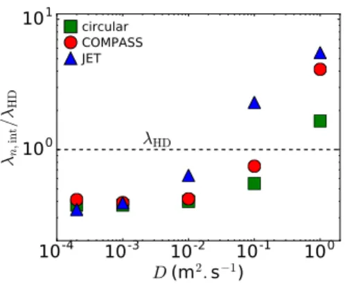
We now compare the value of stagnation λ∇Bwith the HD-model estimate, that is to say a SOL width proportional to

a R

√ T B_pol−1 also obtained in (12). We observe on Fig 9a) that the ratio λ∇B/λHDis approximately constant∼ 2−3 for the three geometries. This

invariable ratio in the three geometry could be explain by the similarity of the parallel equilibrium. Indeed, on Fig 10 reporting the Mach number poloidal SOL profile at a distance λn,intfrom the separatrix, one can observe that the profiles at the LFS coincide for

the three geometry. This interpretation is consistent with the previous assertion that the parallel equilibrium has a strong impact on the establishment of λ in this regime and that the discrepancy with the rough scaling law comes from the assumption of constant parallel speed and parallel length. This also explains that we find about the same ratio for all geometries for the same LFS parallel flows. At the high field side, the parallel flows differs greatly because of the symmetry breaking of divertor configuration : for COMPASS geometry the u_∇B contribution is weaker at the HFS due to the triangularity implying weaker Pfirsch–Schl¨uter flows, on the contrary the circular geometry presents a relatively symmetric parallel profile.

5

Influence of the centrifugal drift

In fluid models, the centrifugal drift is often neglected under the assumption of small mach number in the SOL, ∣ucent∣

∣u∇B∣ = M

2_{<< 1.}

However, we have previously assessed that in ∇B-drift driven simulations supersonic flows are at play, thus neglecting ucent is not

relevant. In this section, the impact of the centrifugal drift on the transverse transport, parallel equilibrium and resulting SOL width is investigated in a JET-like magnetic configuration. For this purpose, we compare simulations including both ∇B and centrifugal drifts with ones including only the ∇B-drift.

(a)

10

₁₀

₁₀

₁₀

₁₀

D

(m

_.

s

)

10

10

λ

(m

m

)

λ

Figure 14 – λn,int and λq,int for ∇B-drift simulations as a function of the diffusion coefficient in anisothermal JET-like simulation

its flux-surface averaged contribution is negligible⟨Γcurv⟩FS/ ⟨Γtot⟩FS< 10%. Contrary to the ∇B-drift flux, the centrifugal drift

flux is not only dependent on the density but also on the parallel flows amplitude. Now, the later presents opposite asymmetry to the one of density, as a result the centrifugal drift has a negligible contribution to the particle flux averaged on a flux-surface. Nevertheless ucent has an indirect impact on the transverse transport, through the modification of the poloidal equilibrium and

⟨Γ∇B,withucent⟩FS ≈ 1.25 × ⟨Γ∇B,withoutucent⟩FS. The plasma equilibrium response to the centrifugal drift is complex, and hard to

capture as it results from a complex inter-play between symmetry breaking of both the parallel velocity and the density, however several effects on the plasma equilibrium and the transverse transport can be underlined.

The first impact of ucentis to stimulate the symmetry breaking. Poloidal profiles present greater variation for Mach number but

also for λn,int(Fig 12 and 5) when it is included in the model. The amplitude of variation in the poloidal direction of λn,int at LFS

for simulation with centrifugal is twice the one for the same simulations without ucent, and the maximum of the Mach number is

1.5 times greater in the case with ucent. Moreover, ucent favors the transition towards supersonic flows which appears at higher D

for simulations including ucent.

This drift has also an impact on radial profiles. At D< Dth, radial profiles exhibit three distinct layers (Fig 13a.) in simulation

including ucent. When moving from the separatrix to the far SOL, one first finds a boundary layer, of about 1.5 mm wide,

characte-rized by flat gradient, followed by a second layer with steeper gradients and finally the last layer with intermediate gradients. The first layer can be interpreted as a thin layer due to the radial displacement via drift convection of particles from the core. Simulations with only ∇B-drift included present also the same kind of pattern although less marked. The second layer is a layer where the transport would be essentially diffusive, in fact the e-folding length in this layer is about the same as the one in simulations without diffusion. The explanation of the third layer is not straightforward, but is most probably link to the rise of the diffusion coefficient at the outer border of the mesh, or to the boundary condition at the wall. Note that this feature is also retrieved at the outer target, with irregular radial profile presenting a flat layer in the area of the strike point.

6

Releasing some assumptions of the model

The previous model addresses explicitly neither the heat transport nor the neutral species. In this section, we further look at the impact of self-consistent electron and ion temperature variations on particles and power SOL width. Simulations are run for two values of thermal diffusivities χi= χe= 1 m2s−1, χi= χe= 0.1 m2s−1, chosen as they are representative of the classical value of

thermal conductivities in the pedestal used in mean field fluid simulations to fit H-mode experiment [20, 21, 22, 23]. Concerning the boundary conditions, the electron and ion temperatures at the inner boundary are taken constant, are equal to 100 eV. On Fig. 14, we observe that, for 1 m2s−1, the value of λn,int as a function of D follows the same trend as in the isothermal simulation,

and the value of saturation of λn,int is similar to the one found in isothermal simulation λn,int = 1.1 mm. Moreover, we find that

λn,int≈ λq,int, under the assumption of high thermal diffusivity. Let us also underline that the equilibrium presents the same feature

than in isothermal simulations, that is to say the presence of supersonic flows and steady-state shock. In the set of anisothermal simulation, the supersonic transition occurs at higher D due to a higher temperature at the separatrix. Simulation have been also run for this χ= 0.1 m2s−1. It is found that the value of λn,int at low D is not impacted, but as we could expect the value of

stagnation of λq,intis smaller but only of about 15%. In this range of χ, the power SOL width are not strongly impacted due to the

fact that λT >> λn. Thus, in the ∇B-drift dominated regime, and for the chosen thermal diffusivities, the assumption that λq ≈ λn

seems reasonable, and the inclusion of temperature variation does not impact drastically the equilibrium.

Finally we study the impact of the inclusion of neutral species in a low recycling regime in the case where only the ∇B-drift is taken into account. Simulations have been run with tungsten PFC for the divertor target and beryllium PFC for outer wall, with recycling coefficients of 0.99 and 1. respectively, the density is set at 1× 1020_m−3 _{at the inner boundary and the density at}

0.0

0.2

0.4

0.6

0.8

1.0

Normalized poloidal distance from LFS divertor target

1

0

1

Mach number

Figure 15 – Mach number poloidal profile in the near SOL, for

∇B-drift simulations for D = 2 × 10−4m2s−1 for simulation

wi-thout neutral species (red with square markers), with neutral spe-cies (black with circle markers)

20

0

20

40

d

(mm)

0.0

0.5

1.0

q/

q

Figure 16 – Heat flux radial profile ∇B-drift simulations at the outer target for D = 2 × 10−4m2_s−1 _{for simulation without (red}

line) and with (black line) the inclusion of neutral species

the separatrix is about 1× 1019_m−3_{in order to be in a low recycling regime (i.e. the framework of the HD-model) and a diffusion}

coefficient is taken equal to 2× 10−4m2_s−1 _{to study the ∇B dominated regime. The inclusion of neutral species is expected to}

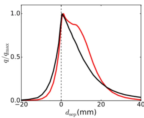
impact the results as it modifies the value of parallel velocity in the divertor region, and we have previously showed that the parallel equilibrium plays a major role in the establishment of the SOL width, indeed Fig. 15 we observe that the inclusion of neutral species results in smaller amplitude of parallel flows, even if a supersonic transition is still reached in this case. This also impacts the parallel variation of density which are of a smaller amplitude and less abrupt. Looking at the profiles at the outer mid-plane, we observe that the simulation including neutral species presents radial profiles with flatter gradient, resulting in a larger SOL width, λn,int= 1.7 mm and λq,int= 1.5 mm. This can be explained by the fact that the Mach number amplitude is lower in the lower-outer

quadrant, so that particles crossing the separatrix at the bottom and flowing toward the top of the machine, are drifting during a longer time, resulting on a larger SOL width at the outer mid-plane. However if we now look at the outer target profile we observe the inverse effect, both density and heat flux profiles of simulation without the inclusion of neutral are more spread than in the case with inclusion of neutral Fig. 16. The detailed study of the physic in the divertor region is out of the scope of this paper, but let us mention several mechanisms that can explain this effect. First it is important to underline that the repartition of particle sources is completely modified, and the ionization of neutrals in the divertor region become a major player in the source for the plasma. This tends to decouple the physic of the main SOL and divertor explaining that we observe opposite variation of the profile in the two regions. This effect can also be observed in the parallel flow amplitude, in simulations without neutral only a thin boundary layer at the vicinity of the separatrix presents a Mach number close to zeros, when in simulation with neutral the Mach number is close to zero at the divertor entrance on all the radial domain of the SOL. The fact the radial profile at the outer target presents sharper gradients at the strike point in the case including neutrals could be partly due to ionization. Indeed this mechanism is proportional to the local density, so will be maximum at the strike point, this way reinforcing the plasma source at the peak location.

7

Comparison of the results with the heuristic-drift based model and discussion

on its hypothesis

The reduced model used in the section 3, corresponds to the main assumption made in the heuristic drift based model. Hence, it is worth comparing λn,Eich with the one predicted by the HD-model λHD = 2

√ 2a_(B B

pR)MP

ρL. The numerical application for

the JET geometry gives λHD≈ 3 mm namely twice the limit found in simulations limD→0λn,Eich≈ 1.5 mm. Let us recall that this

discrepancy between our numerical results and the HD-model estimate is also retrieve for the other geometries (section 4). Moreover, the functional dependency on T (λHD ∝

√

T ) is not retrieve in our simulations. The scaling in Bpol, although it shows a better

agreement with the model, is not unquestionable. Indeed, the dependency seems to be weaker than predicted, as highlighted by the lower Bpol point, showing a variation 40% lower than the HD-model prediction Fig. 7b).

The discrepancy between numerical results and the model is readily explainable by the parallel equilibrium, important in the establishment of the SOL width in the drift dominated regime. Indeed, the reduced model predicts λn,Eich under the assumption

that the parallel velocity is constant and equal to cs/2 in the lower outer quadrant of the SOL, while the Mach number at low

diffusion varies between -cs and cs in this poloidal extent (Fig 3). Moreover, it assumes that particles flow from the outer target

to the entry of the divertor when in low diffusion simulations the stagnation point is halfway between the outer mid-plane and the X-point so particles crossing the separatrix at the outer mid-plane flow to the top of the machine and not downward to the divertor

target. In conclusion, within the main hypothesis of the model, the assumption of a ∇B-drift dominated regime seems to lead to a contradiction with the first heuristic made that ”the parallel flow along B to the divertor competes at order unity with the usual Pfirsch–Schl¨uter parallel flow to the opposite side of the plasma” [11].

One should also keep in mind that some physics missing in the HD-model, is proven to play an important role in the plasma equilibrium. First, the centrifugal drift is implicitly neglected in this model under the assumption that u_∥/cs≈ 0.5. However, we

have showed, on the contrary to this assumption, the ∇B-drift dominated regime is characterised by large amplitude flows and that ucent plays a role in the establishment of the equilibrium section 5. Furthermore, the HD-model addresses explicitly neither

the heat transport nor the neutral species. If the assumption, that the thermal transport is fast enough so that λn ≈ λq seems to

be valid considering the classical diffusivity used in the pedestal, the impact of the neutrals species should be taken into account as it impacts significantly both the equilibrium and the profiles.

The study of the charge balance is out of the scope of this work, and is a hard task from a numerical point of view due to the complexity of the equilibrium presenting stationary shock and sharp gradients. However, we know that the ∇B drifts are charge dependent, and in the ∇B-drift dominated regime, the principal mechanism of transport leads to a charge separation and must therefore drives significant electric fields. Moreover, it has been shown that the electric drift has not only an importance in E× B turbulence but also drives large scale transport that need to be taking into account even for a laminar approach [27]. Due to numerical constraint, too demanding in the regime of low D considered here, no simulation including the drift E× B have been run yet. However, one could expect a strong effect of the addition of the drift, especially in the low anomalous transport regime. Indeed, for a quasi-adiabatic electric field model, one has φ(θ) ∝ ln N (θ). Considering the large poloidal inhomogeneities of density, it would create a large ∂θφ, i.e. a large radial E× B drift velocity urE. Such E× B flows could modify significantly the equilibrium.

8

Conclusions

In this work, we have studied the impact of the ∇B-drift on the cross-field transport and on the SOL’s width for different levels of anomalous transport using the fluid code SolEdge2D. The first conclusion of this work is that in all cases, including anisothermal simulations and simulation taking account neutral species, and all geometries a ∇B-drift dominated regime is reach at low D. In this regime the value of SOL particles or power width is set by the magnetic drift and does not depend on D. However the relevance of this regime is disputable as it exists only at very low anomalous and collisional transport, well below the neoclassical level. This result is in agreement with the previous works of [15, 16], note that in [16] this regime appears at higher D, but this difference can be explained by the parameters of the simulations, in particular a higher temperature at the inner boundary of Te= Ti= 500 eV

against a range of temperature of 50 eV to 100 eV used in this work. If we reach in all case the ∇B-drift dominated regime, the resulting SOL widths are significantly lower, of a factor comprise between 2 and 3, than the estimate of HD-model. Moreover, the parametric functional dependencies of the estimate, in particular the one on T , are not retrieved.

An other robust conclusion is that the ∇B-drift dominated regime and the saturation of SOL width are linked to the transition toward a complex poloidal equilibrium, characterized by the apparition of supersonic flow and steady-state shock. This appearance of a supersonic transition is supported by a simple 1D-analytical model, which have shown good agreement with numerical simulations. Moreover, the parallel equilibrium seems to plays a role in the establishment of the SOL width, and it provides a reasonable explanation for the discrepancies between the estimate of HD-model and the numerical results. Hence, a reduce model for the drift dominated regime should take into account the complexity of the parallel equilibrium. Furthermore, in this regime characterized by large Mach number amplitude, the impact of the centrifugal drift should be explicitly taking into account, as we have proven in section 5 that the inclusion of this drift impact significantly the equilibrium of the plasma.

Finally, one should discuss some open remaining questions. Especially in this work we have not included the E×B drift, however it has been shown that the electric drift has not only an importance in E× B turbulence but also drives large scale transport that need to be taken into account even for a laminar approach [27]. Moreover, here the charge balance are not taking into account. Considering the large asymmetry at play in the simulations at low anomalous transport one could expect large potential response, thus large E× B flows modifying significantly the equilibrium.

R´

ef´

erences

[1] A Loarte, B Lipschultz, AS Kukushkin, GF Matthews, PC Stangeby, N Asakura, GF Counsell, G Federici, A Kallenbach, K Krieger, et al. Power and particle control. Nuclear Fusion, 47(6) :S203, 2007.

[2] T Eich, B Sieglin, A Scarabosio, W Fundamenski, RJ Goldston, A Herrmann, and ASDEX Upgrade Team. Inter-elm power decay length for jet and asdex upgrade : Measurement and comparison with heuristic drift-based model. Physical review letters, 107(21) :215001, 2011.

[3] T Eich, B Sieglin, A Scarabosio, A Herrmann, A Kallenbach, GF Matthews, S Jachmich, S Brezinsek, M Rack, RJ Goldston, et al. Empiricial scaling of inter-elm power widths in asdex upgrade and jet. Journal of Nuclear Materials, 438 :S72–S77, 2013.

[4] Thomas Eich, AW Leonard, RA Pitts, W Fundamenski, RJ Goldston, TK Gray, A Herrmann, A Kirk, A Kallenbach, O Kar-daun, et al. Scaling of the tokamak near the scrape-off layer h-mode power width and implications for ITEr. Nuclear Fusion, 53(9) :093031, 2013.

[5] AJ Thornton, A Kirk, MAST Team, et al. Scaling of the scrape-off layer width during inter-elm h modes on mast as measured by infrared thermography. Plasma Physics and Controlled Fusion, 56(5) :055008, 2014.

[6] H J Sun, E Wolfrum, T Eich, B Kurzan, S Potzel, U Stroth, and the ASDEX Upgrade Team. Study of near scrape-off layer (sol) temperature and density gradient lengths with thomson scattering. Plasma Physics and Controlled Fusion, 57(12) :125011, 2015.

[7] A Scarabosio, T Eich, A Herrmann, B Sieglin, JET-EFDA contributors, et al. Outer target heat fluxes and power decay length scaling in l-mode plasmas at jet and aug. Journal of Nuclear Materials, 438 :S426–S430, 2013.

[8] JP Gunn, R Dejarnac, P Devynck, N Fedorczak, V Fuchs, C Gil, M Koˇcan, M Komm, M Kubiˇc, T Lunt, et al. Scrape-off layer power flux measurements in the tore supra tokamak. 438 :S184–S188.

[9] Paolo Ricci and BN Rogers. Transport scaling in interchange-driven toroidal plasmas. Physics of Plasmas, 16(6) :062303, 2009.

[10] Nicolas Fedorczak, JP Gunn, N Nace, A Gallo, C Baudoin, H Bufferand, G Ciraolo, Th Eich, Ph Ghendrih, and Patrick Tamain. Width of turbulent sol in circular plasmas : a theoretical model validated on experiments in tore supra tokamak. Nuclear Materials and Energy, 12 :838–843, 2017.

[11] RJ Goldston. Heuristic drift-based model of the power scrape-off width in low-gas-puff h-mode tokamaks. Nuclear Fusion, 52(1) :013009, 2012.

[12] FL Hinton and RD Hazeltine. Kinetic theory of plasma scrape-off in a divertor tokamak. Physics of Fluids (1958-1988), 17(12) :2236–2240, 1974.

[13] M Faitsch, B Sieglin, T Eich, HJ Sun, and A Herrmann. Change of the scrape-off layer power width with the toroidal b-field direction in asdex upgrade. Plasma Physics and Controlled Fusion, 57(7) :075005, 2015.

[14] B Sieglin, T Eich, M Faitsch, A Herrmann, D Nille, A Scarabosio, and ASDEX Upgrade Team. Density dependence of sol power width in asdex upgrade l-mode. Nuclear Materials and Energy, 2016.

[15] D Reiser and T Eich. Drift-based scrape-off particle width in x-point geometry. Nuclear Fusion, 57(4) :046011, 2017.

[16] ET Meier, RJ Goldston, EG Kaveeva, MA Makowski, S Mordijck, VA Rozhansky, I Yu Senichenkov, and SP Voskoboynikov. Analysis of drift effects on the tokamak power scrape-off width using solps-ITEr. Plasma Physics and Controlled Fusion, 58(12) :125012, 2016.

[17] AV Chankin and DP Coster. The role of drifts in the plasma transport at the tokamak core–sol interface. Journal of Nuclear Materials, 438 :S463–S466, 2013.

[18] Hugo Bufferand, Guido Ciraolo, Yannick Marandet, J´erome Bucalossi, Ph Ghendrih, Jamie Gunn, N Mellet, Patrick Tamain, R Leybros, Nicolas Fedorczak, et al. Numerical modelling for divertor design of the west device with a focus on plasma–wall interactions. Nuclear Fusion, 55(5) :053025, 2015.

[19] AV Chankin. Classical drifts in the tokamak sol and divertor : models and experiment. Journal of nuclear materials, 241 :199– 213, 1997.

[20] AV Chankin, DP Coster, R Dux, Ch Fuchs, G Haas, A Herrmann, LD Horton, A Kallenbach, M Kaufmann, Ch Konz, et al. Solps modelling of asdex upgrade h-mode plasma. Plasma physics and controlled fusion, 48(6) :839, 2006.

[21] LD Horton, AV Chankin, YP Chen, GD Conway, DP Coster, T Eich, E Kaveeva, C Konz, B Kurzan, J Neuhauser, et al. Characterization of the h-mode edge barrier at asdex upgrade. Nuclear fusion, 45(8) :856, 2005.

[22] A Kallenbach, Y Andrew, M Beurskens, G Corrigan, T Eich, S Jachmich, M Kempenaars, A Korotkov, A Loarte, G Matthews, et al. EDGE2D modelling of edge profiles obtained in jet diagnostic optimized configuration. Plasma physics and controlled fusion, 46(3) :431, 2004.

[23] B. Gulejov´a, R.A. Pitts, M. Wischmeier, R. Behn, D. Coster, J. Horacek, and J. Marki. Solps5 modelling of the type iii elming h-mode on tcv. Journal of Nuclear Materials, 363 :1037–1043, 2007. Plasma-Surface Interactions-17.

[24] W Fundamenski, Odd Erik Garcia, Volker Naulin, RA Pitts, Anders Henry Nielsen, J Juul Rasmussen, J Horacek, JP Graves, et al. Dissipative processes in interchange driven scrape-off layer turbulence. Nuclear fusion, 47(5) :417, 2007.

[25] Ph Ghendrih, K Bodi, H Bufferand, Guillaume Chiavassa, Guido Ciraolo, Nicolas Fedorczak, Livia Isoardi, A Paredes, Ya-nick Sarazin, Eric Serre, et al. Transition to supersonic flows in the edge plasma. Plasma Physics and Controlled Fusion, 53(5) :054019, 2011.

[26] M Koˇcan, RA Pitts, G Arnoux, I Balboa, PC de Vries, R Dejarnac, I Furno, RJ Goldston, Y Gribov, J Horacek, et al. Impact of a narrow limiter sol heat flux channel on the ITEr first wall panel shaping. Nuclear Fusion, 55(3) :033019, 2015.

[27] D. Galassi, P. Tamain, H. Bufferand, G. Ciraolo, Ph. Ghendrih, C. Baudoin, C. Colin, N. Fedorczak, N. Nace, and E. Serre. Drive of parallel flows by turbulence and large-scale e× b transverse transport in divertor geometry. Nuclear Fusion, 57(3) :036029, 2017.