HAL Id: hal-03090960
https://hal.archives-ouvertes.fr/hal-03090960
Submitted on 30 Dec 2020
HAL is a multi-disciplinary open access
archive for the deposit and dissemination of sci-entific research documents, whether they are pub-lished or not. The documents may come from teaching and research institutions in France or abroad, or from public or private research centers.
L’archive ouverte pluridisciplinaire HAL, est destinée au dépôt et à la diffusion de documents scientifiques de niveau recherche, publiés ou non, émanant des établissements d’enseignement et de recherche français ou étrangers, des laboratoires publics ou privés.
Analysis, improvement and limits of the multiscale Latin
method
Paul Oumaziz, Pierre Gosselet, Karin Saavedra, Nicolas Tardieu
To cite this version:
Paul Oumaziz, Pierre Gosselet, Karin Saavedra, Nicolas Tardieu. Analysis, improvement and limits of the multiscale Latin method. Computer Methods in Applied Mechanics and Engineering, Elsevier, 2021, 384, pp.113955. �10.1016/j.cma.2021.113955�. �hal-03090960�
Analysis, improvement and limits of the multiscale Latin method
Paul Oumaziz1,2, Pierre Gosselet3,4, Karin Saavedra5, Nicolas Tardieu6
1 Núcleo Científico Multidisciplinario, Facultad de Ingeniería, Universidad de Talca, Campus Curicó, Chile
2 Institut Clément Ader (ICA), Université de Toulouse, CNRS/INSA/ISAE/Mines Albi/UPS - 3 rue Caroline Aigle, 31 400 Toulouse, France
3 Univ. Lille, CNRS, Centrale Lille, UMR 9013 - LaMcube - Laboratoire de Mécanique, Multiphysique, Multiéchelle, F-59000 Lille, France
4 LMT, ENS Paris-Saclay/UMR 8535 CNRS/Université Paris-Saclay - 4, avenue des Sciences 91190 Gif-sur-Yvette, France
5 Dpto. Tecnologías Industriales, Facultad de Ingeniería, Universidad de Talca, Campus Curicó, Chile 6 IMSIA, UMR 9219 EDF-CNRS-CEA-ENSTA, Saclay, France
Abstract
This work studies the convergence properties of the mixed non-overlapping domain decomposition method (DDM) commonly named “Latin method”. As all DDM, the Latin method is sensitive to near-interface heterogeneity and irregularity. Using a simple yet fresh point of view, we analyze the role of the Robin parameters as well as of the second level (coarse space) correction – which are a characteristic of the method. In particular, we show how to build a spectrum-motivated coarse space aiming at ensuring fast convergence. 2D and 3D linear elasticity problems involving highly heterogeneous materials confirm the robustness of the spectral coarse space and provide evidence of the scalability of the multiscale Latin method.
Keywords Latin method, domain decomposition method, spectral coarse problem, GenEO, heteroge-neous problem
1
Introduction
Domain Decomposition Methods [1] (DDM) offer a powerful framework to design efficient parallel iterative solvers for computational mechanics problems. Recently, much progress has been made in understanding the methods and how to make them robust, in particular with respect to misplaced heterogeneity and poorly shaped subdomains.
The first possibility consists in using a preprocessing step where local generalized eigenvalue problems detect “bad” spectral contributions. These harmful components are then removed from the resolution process by adding constraints to the system. In FETI-DP (Dual-Primal Finite-Element Tearing and Interconnection) or BDDC (Balancing Domain Decomposition by Constrains) methods, the constraints can be applied by selecting the coarse degrees of freedom [2, 3, 4, 5, 6, 7, 8]. In FETI and BDD methods, Krylov-augmented solvers are used to remove the bad modes which have been detected by a technique inspired from Schwarz methods (see [9, 10, 11, 12, 13] and references therein) and known as “Generalized Eigenvalue problems in the Overlap” (GenEO) [14, 15, 16, 17]. GenEO coarse spaces were also extended to the Symmetrized Optimized Restricted Additive Schwarz (SORAS) algorithm [18, 19].
The second alternative is to rely on a multipreconditioned solver [20]. This was proposed for the FETI method in [21] where as many search directions as subdomains are generated by the conjugate gradient at each iteration. Less demanding versions were presented in [22] and illustrated in [23]. Note that a link between multipreconditioning and GenEO coarse spaces was exhibited in [24].
This paper is devoted to the Latin DDM [25]. This strategy makes use of mixed (Robin) interface conditions, it was specifically designed to solve nonlinear mechanical problems involving complex behaviors inside subdomains and on their interfaces by stationary iterations, and it has been successfully applied to viscoplasticity, frictional contact, cracking, cohesive interfaces [26, 27, 28, 29, 30, 31] and also naturally coupled with the PGD (Proper Generalized Decomposition) model reduction [32, 33]. In [34], a two-level version was proposed to grant a certain scalability face to moderate heterogeneity. Note that in [35, 36] the authors proposed an analysis of the method in the light of more classical domain decomposition methods, and showed how a simple non-invasive implementation using python and MPI to pilot an industrial finite element software (code-aster [37] in this case)
Here, we propose to analyze the multiscale Latin approach and try to apply the GenEO philosophy. We show that local generalized eigenvalue problems naturally arise when studying the convergence of the Latin DDM. For a chosen convergence ratio, it is then possible to tell “nefarious” eigenvectors from “innocuous” ones, opening the path to sounder higher-order coarse spaces than the ones commonly based on polynomial development of interface quantities. Unfortunately, we show that in current state, the multiscale Latin approach does not permit to precisely remove the unwanted components and parasitic effects cannot be prevented.
The article is organized as follows: Section 2 introduces notations and the substructured problem, Section 3 presents the monoscale Latin method which is then analyzed in Section 4 through a generalized eigenvalue problem. Section 5 is dedicated to the multiscale (or two-level) approach, and we show how a hopefully efficient coarse space can be built from previously obtained eigenvector. Finally, Section 7 illustrates the method on three highly heterogeneous academic test-cases.
2
The problem to be solved in substructured form
A domain Ω ∈ Rd (d = 2 or 3) under small perturbations and quasi-static isotherm evolution is considered, the material is supposed to be linear elastic and classical Lagrange conforming finite element is used to approximate the displacement field.
2.1 Subdomains equations
We take into account a non-overlapping decomposition of N subdomains (Ω(s))
S∈N. For the subdomain Ω(s), let K(s) denote the stiffness matrix, u(s) the vector of nodal displacement and g(s) the generalized forces associated to given loads, including the forces resulting from the elimination of Dirichlet boundary conditions. Matrix K(s) is symmetric semi-definite positive, the null space is spanned by rigid body motions for floating subdomains.
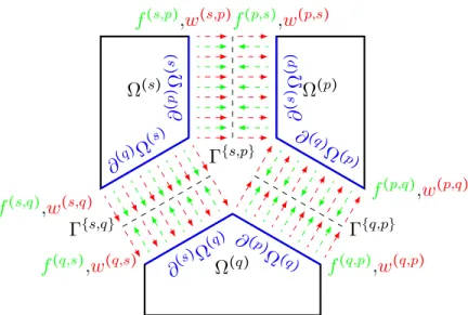
Let Ω(s) and Ω(q) be two neighbors subdomains. We write ∂(q)Ω(s) the degrees of freedom of Ω(s) facing Ω(q). Some degrees of freedom can be shared by two boundaries, see Figure 1. Boundaries ∂(q)Ω(s) and ∂(s)Ω(q) interact through the interface Γ{s,q}=∂Ω(s)∩∂Ω(q). The interface Γ{s,q} is granted its own finite element discretization, while displacements and reactions associated with each parent subdomains are defined as (w(s,q), w(q,s)
) and (f(s,q), f(q,s)), respectively. These fields are connected to the parent subdomains by trace relations materialized by the operators N(s,q) and N(q,s). For now, we consider conforming discretization between the subdomains (Ω(s), Ω(q)) and the interface Γ{s,q}, so that the trace operators are simple boolean matrices. Let G(s)be the set of the neighbors of the subdomain Ω(s); E the set of all subdomains and G the set of all interfaces.
Ω
(s)Ω
(q)Ω
(p)f
(p,s),
w
(p,s)f
(s,p),
w
(s,p)f
(s,q),
w
(s,q)f
(q,s),
w
(q,s)f
(q,p),
w
(q,p)f
(p,q),
w
(p,q)Γ
{s,q}Γ
{q,p}Γ
{s,p}∂
( p )Ω
( s )∂
( s )Ω
( p )∂
(q )Ω
(s)∂
(q)Ω
(p )∂
(s )Ω
(q)∂
(p)Ω
(q )Figure 1: Force and displacement interface fields.
To easily handle the many interfaces of one subdomain Ω(s), we define concatenated operators: w(s)= ⎛ ⎜ ⎝ ⋮ w(s,q) ⋮ ⎞ ⎟ ⎠ , f(s)= ⎛ ⎜ ⎝ ⋮ f(s,q) ⋮ ⎞ ⎟ ⎠ , N(s)= ⎛ ⎜ ⎝ ⋱ N(s,q) ⋱ ⎞ ⎟ ⎠ , q ∈ G(s) (1)
Thus, the mechanical problems to be solved on the subdomains can be written as follows: On subdomains: ∀Ω(s) ∈ E, ⎧ ⎪ ⎪ ⎨ ⎪ ⎪ ⎩ K(s)u(s)=g(s)+N(s) T f(s) w(s)=N(s)u(s) (2) Remark 1 (Condensation). Since the interface vectors are only connected to the boundary of the subdo-mains, we tag with index b the boundary degrees of freedom of the subdomain and the trace relationship can be written as:
∀Ω(s)∈ E, w(s)=N(s)
b u
(s)
b (3)
Also, internal nodes (index i) can be eliminated from the balance of the domain leading to the condensed form of the equilibrium:
∀Ω(s)∈ E, S(s)u(s)b =b(s)+N(s) T b f (s) (4) where S(s)=K(s) bb −K (s) bi K (s)−1 ii K (s)
ib is the Schur complement and b
(s)=g(s) b −K (s) bi K (s)−1 ii giis the condensed right-hand side. Proposition 1 (Properties of N(s)b ). N(s)b is a n(s)Γ ×n(s) ∂ matrix, where n (s)
∂ is the number of boundary degrees of freedom of Ω(s) and n(s)Γ is the number of interface degrees of freedom of (Γ{s,q})q∈G(s). In the presence of multiple points (node facing more than one neighbor), n(s)Γ >n(s)∂ and the matrix is not full-ranked, see Figure 1.
2.2 Interfaces equations
The mechanical behavior of the interface Γ{s,q}is given by a relationship which links the boundary vectors (w(s,q), w(q,s), f(s,q), f(q,s)). Many mechanical behaviors, such as perfect interfaces, contact, friction or loss of cohesion can be represented by constraining the force to belong to a domain of admissibility –
materialized by a function c– which depends on the displacement gap and satisfies the action-reaction principle: On general interfaces: ∀Γ{s,q}∈ G, ⎧ ⎪ ⎪ ⎨ ⎪ ⎪ ⎩ f(s,q)∈c(s,q)(w(s,q)−w(q,s)) f(s,q)+f(q,s)=0 (5) Note that internal variables could be incorporated into relation c to transcribe history-dependent behaviors like friction or debonding. However, in this work we only take into account perfect interfaces by stating the continuity of the displacement, then Equation (5) becomes:
On perfect interfaces: ∀Γ{s,q} ∈ G, ⎧ ⎪ ⎪ ⎨ ⎪ ⎪ ⎩ w(s,q)=w(q,s) f(s,q)+f(q,s)=0 (6)
2.3 Assembly operators and interface behaviors
Block notations are also here employed. For instance, vectors are concatenated by rows and matrices on the diagonal as follows:
u = ⎛ ⎜ ⎝ ⋮ u(s) ⋮ ⎞ ⎟ ⎠ , K = ⎛ ⎜ ⎝ ⋱ 0 K(s) 0 ⋱ ⎞ ⎟ ⎠ , s ∈ E (7)
This leads to the following expression being equivalent to Equation (2): On subdomains: {Ku = g + N
Tf
w = Nu (8)
We introduce assembly operators for communicating neighboring subdomains. Operator A makes the sum of interface vectors whereas operator B makes the difference (an arbitrary orientation is chosen on the interface):
(Af )∣Γ{s,q}=f(s,q)+f(q,s) (Bw)∣Γ{s,q}=w(s,q)−w(q,s)
(9) Proposition 2 (Properties of interface operators). Operators A and B are nΓ×2nΓ matrices, where nΓ= ∑s<qnΓ{s,q} is the number of all interface degrees of freedom. They are full-ranked operators and also are orthogonal in the sense that:
ker(A) = range(BT) (10)
This implies that ABT =0. More precisely, any interface vector x can be written uniquely under the form x = ATxA+BTxB. In fact, this property can be generalized using non-euclidean orthogonality. Let Q be any symmetric positive definite matrix of size 2nΓ, then we have:
R2nΓ = (Q Range(AT)) ⊕Range(BT) (11)
Finally, assembly operators enable to easily write the perfect interface behavior as follows: On perfect interfaces: {Af = 0
Bw = 0 (12)
Note that the general case takes the form f = BTc(Bw). This notation makes it clear that the interface equilibrium is satisfied since Af = ABTc(Bw) = 0. For instance, the contact formulation with Coulomb friction is fully detailed in [35].
2.4 Partial solutions and total solution
The interface fields are gathered in two sets:
A ∶ (w, f )solutions to ∃u/ {Ku = g + N Tf w = Nu ⇔ ∃ub/ { Sub=b + NTbf w = Nbub (13) L ∶ ( ̂w,̂f )solutions to { Âf = 0 B ̂w = 0 (14)
The set A generally called admissibility space is the affine space made out of the solutions to the linear equations on the subdomains, i.e. the equilibrium of the subdomains submitted to the given load. The set L of solutions to the interface equations is called local space; it is a vector space in the case of perfect interfaces, it would be a cone for Coulomb friction or a manifold for more complex interface behaviors. Remark 2. Note that this framework extends to many mechanical situations, including time-dependent problems, nonlinear behaviors in the volume or large transformations, as long as A is characterized by linear equations (potentially associated with differential operators) and L is defined by non-differential equations (potentially nonlinear).
Of course, if (w, f) ∈ L ∩ A then (w, f) solves the whole substructured formulation. Note that w is defined uniquely but f is not as stated is the next proposition.
Proposition 3 (Indeterminacy of f). In the presence a multiple points, the subspace ker(NTbBT) is not reduced to 0. This means that there exist balanced interface force (of the form f = BTβ) which result in the same mechanical effort NTbf on the subdomains. This phenomenon is very well-known in FETI methods, and in practice it does not bring any difficulty.
3
The monoscale Latin method
3.1 Principle
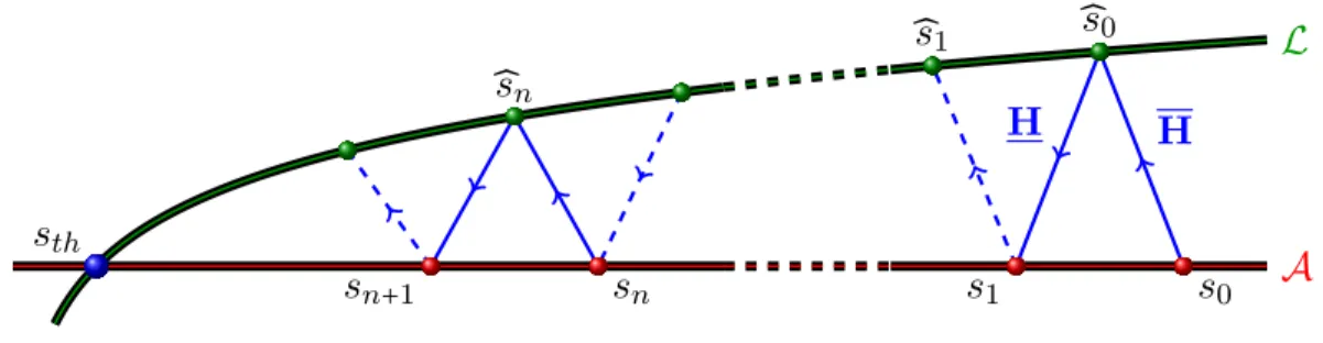
The Latin method is an alternating direction algorithm. Solution (w, f) is reached through partial solutions of the sets A and L, which are consecutively calculated as illustrated in Figure 2.
A
L
H
̂
s
0H
̂
s
1s
0s
1s
ns
n+1̂
s
ns
thFigure 2: Illustration of the Latin framework.
Firstly, starting from a partial solution sn= (wn, fn) ∈ A, the so-called local stage consists in searching for a partial solution ̂sn= ( ̂wn,̂fn) ∈ L. This is possible by enforcing a relation of the form:
̂f
n−fn−H ( ̂wn−wn) =0 (15)
This equation is often called “local search direction” in the Latin literature. H is a symmetric definite positive operator selected by the user, however, for computational efficiency – in particular in the case of complex interface behaviors – it should be chosen to be diagonal.
Then, starting from a partial solution ̂sn= ( ̂wn,̂fn) ∈ L, the so-called linear stage consists in searching for a partial solution sn+1= (wn+1, fn+1) ∈ A. This is possible by enforcing a relation of the form:
fn+1− ̂fn+H (wn+1− ̂wn) =0 (16)
This equation is often called “linear search direction”, where H is also a symmetric definite positive operator chosen by the user.
3.2 The local stage
The local stage finds a partial solution of the equations defined on the interfaces by enforcing the search direction. Then, the problem to be solved is:
Knowing sn= (wn, fn), find ̂sn= ( ̂wn,̂fn)/ ⎧ ⎪ ⎪ ⎪ ⎪ ⎨ ⎪ ⎪ ⎪ ⎪ ⎩ Âfn=0 B ̂wn=0 ̂f n−fn−H ( ̂wn−wn) =0 (17) which gives the following solution:
⎧ ⎪ ⎪ ⎪ ⎨ ⎪ ⎪ ⎪ ⎩ ̂ wn=AT(AHAT)−1[AHwn−Afn] ̂f n=BT (BH−1BT) −1 [BH−1fn−Bwn] (18) We recognize scaled assembly operators as classically encountered in FETI and BDD methods [38, 39]:
̂ A = (AHAT) −1 AH ̂ B = (BH−1BT) −1 BH−1 (19)
They satisfy ÂAT =I, B̂BT =I and ATA + ̂̂ BTB = I[40].
The set L gathers interface equations, and thus, compared to the complete system to be solved, it misses the subdomain mechanical behavior. H should provide a computationally affordable ersatz of this information. To make this analysis precise, let us use the condensed form of A to express w and f in terms of ub.
̂f
n−fn−H ( ̂wn−wn) =0 ⇒ NTb̂fn− (Sub,n−b) − NTbH ( ̂wn−wn) =0 ⇒ (NTbHNb−S) ub,n− (NTbH ̂wn−NTb̂fn−b)
(20) Proposition 4 (Optimal local search direction). If H is such that NTbHNb=S, then the system formed by the above equation and the interface conditions (14) is equivalent to the substructured problem. In that case, the local stage directly gives the exact solution.
Let ̃Nb be a matrix such that NTbÑb = I, such as for instance ̃Nb = Nb(NTbNb)−1, and let ̃S be an approximation of S (like a weighted superlumped operator). We thus should choose H = diag ( ̃Nb̃S ̃NTb). In the case of ̃Nb=Nb(NTbNb)−1, this accounts to weighting diag(̃S) by the inverse of the multiplicity of the interface nodes (number of interfaces a boundary nodes textcolororangenode belongs to).
3.3 The linear stage
The linear stage finds a partial solution verifying the equilibria of subdomains while respecting the search directions. This leads to the following problem set independently on subdomains:
Knowing ̂sn= ( ̂wn,̂fn), find sn+1= (w, f )/ ⎧ ⎪ ⎪ ⎪ ⎪ ⎨ ⎪ ⎪ ⎪ ⎪ ⎩ Kun+1=g + NTfn+1 wn+1=Nun+1 fn+1− ̂fn+H (wn+1− ̂wn) =0 (21)
leading as follows:
Solve for un+1 solution to: (K + NTHN) un+1=g + NT(̂fn+H ̂wn) Then compute: ⎧ ⎪ ⎪ ⎨ ⎪ ⎪ ⎩ wn+1=Nun+1 fn+1= ̂fn+H ( ̂wn−wn+1) (22) 3.4 Relaxation
To ensure convergence [25] a relaxation step is added at the end of a linear stage, thus:
sn+1←Ðωsn+1+ (1 − ω) sn (23)
The method is proved to converge in a very general framework (including nonlinear behavior associated with a convex potential) assuming that relaxation is used and that search directions are chosen to be equal H = H.
3.5 Other choices of search directions
Selecting the search directions is crucial for the convergence ratio of the algorithm. In Section 3.2 we have proposed approximations of the optimal one for the local stage, but we can also raise the possibility of search directions motivated by a FETI preconditioner [39]. In that case, the same direction is used for both stages, written H and defined as a scaled assembly of approximate subdomains stiffness. Additionally, the same value is employed for the two subdomains connected by an interface. Therefore, the common linear/local search direction can be written as:
H = 1 2(A
THA + B̃ THB)̃ (24)
where ̃H = (ADAT)−1ADMDAT(ADAT)−1 is an operator defined on the interfaces, D a diagonal matrix and M a block-diagonal matrix. The operator AT⋯A+BT⋯B
2 brings back ̃Hto the boundary of the subdomains.
In practice, inspired by FETI scaling and preconditioners, we propose to use D = ̃Nbdiag (Kbb)−1ÑTb, whereas two possible alternatives regarding M:
• M = ̃Nbdiag (S)−1ÑTb, leading to a search direction named HS. • M = D+, leading to the search direction H
K =AT(ADAT)−1A.
4
Analysis of the monoscale method
In this section, the Latin method is recast into a fixed-point iteration and a convergence analysis is then derived. This allows to recover some classical properties of the algorithm and to introduce better decisions for a multiscale extension.
Because the equations of perfect interfaces are linear, we can rewrite both linear and local stages in a matrix form with the interface unknown (wn, fn) and (̂wn,̂fn) as the variables, where index n stands for the iteration counter. In fact, the local stage (18) can be written as:
( ̂ wn ̂f n ) = (A TÂ 0 0 BTB̂) ( H−1 −I ) (H −I) (wn fn ) (25)
while the linear stage (22) can be formulated like this: (wn+1 fn+1 ) = (w0 f0 ) + ( I 0 −H I ) (N (K + N THN)−1NT I ) (H I) ( ̂ wn ̂f n ) (26)
where, we have named the following quantity: (w0 f0 ) = ( I −H)N (K + N THN)−1g
At last, if we introduce the mixed variable µn=Hwn−fn, the iteration takes the form µn+1=µ0+Mµn, where the iteration matrix M can be written as:
M = (H −I) ( I 0 −H I ) (N (K + N THN)−1NT I ). . . . . . (H I) (A TÂ 0 0 BTB̂) ( H−1 −I ) (27) Using the expression of the scaling matrices (19) and their properties, it simplifies to:
M = ((H + H) N (K + NTHN)−1NT −I) (HATAĤ −1−BTB)̂ = ((H + H) N (K + NTHN) −1 NT −I) ´¹¹¹¹¹¹¹¹¹¹¹¹¹¹¹¹¹¹¹¹¹¹¹¹¹¹¹¹¹¹¹¹¹¹¹¹¹¹¹¹¹¹¹¹¹¹¹¹¹¹¹¹¹¹¹¹¹¹¹¹¹¹¹¹¹¹¹¹¹¹¹¹¹¹¹¹¹¹¹¹¹¹¹¹¹¹¹¹¹¹¹¹¹¹¹¹¹¹¹¹¹¹¹¹¹¹¹¹¹¹¹¹¹¹¹¹¹¹¹¹¹¹¹¹¹¸¹¹¹¹¹¹¹¹¹¹¹¹¹¹¹¹¹¹¹¹¹¹¹¹¹¹¹¹¹¹¹¹¹¹¹¹¹¹¹¹¹¹¹¹¹¹¹¹¹¹¹¹¹¹¹¹¹¹¹¹¹¹¹¹¹¹¹¹¹¹¹¹¹¹¹¹¹¹¹¹¹¹¹¹¹¹¹¹¹¹¹¹¹¹¹¹¹¹¹¹¹¹¹¹¹¹¹¹¹¹¹¹¹¹¹¹¹¹¹¹¹¹¹¹¹¶ M1 ((H + H)AT(AHAT)−1A − I) ´¹¹¹¹¹¹¹¹¹¹¹¹¹¹¹¹¹¹¹¹¹¹¹¹¹¹¹¹¹¹¹¹¹¹¹¹¹¹¹¹¹¹¹¹¹¹¹¹¹¹¹¹¹¹¹¹¹¹¹¹¹¹¹¹¹¹¹¹¹¹¹¹¹¹¹¹¹¹¹¹¹¹¹¹¹¹¹¹¹¹¹¹¹¹¹¹¹¹¹¹¹¸¹¹¹¹¹¹¹¹¹¹¹¹¹¹¹¹¹¹¹¹¹¹¹¹¹¹¹¹¹¹¹¹¹¹¹¹¹¹¹¹¹¹¹¹¹¹¹¹¹¹¹¹¹¹¹¹¹¹¹¹¹¹¹¹¹¹¹¹¹¹¹¹¹¹¹¹¹¹¹¹¹¹¹¹¹¹¹¹¹¹¹¹¹¹¹¹¹¹¹¹¹¹¶ M2 (28)
The iteration matrix can thus be written as the product of two matrices of which we suggest analyze the spectrum under the next hypotheses:
Hypothesis 1 (Same assembled search directions). AHAT =AHAT.
Hypothesis 2 (Identical search directions). H = H, in that case we use the notation H for both directions. Of course, Hypothesis 2 is stronger than Hypothesis 1.
Proposition 5 (Spectrum of matrix M2). Under Hypothesis 1, the spectrum of Matrix M2 is exactly {−1, 1} and thus the spectral radius is 1.
Proof. Let be xT = (xTAA + xTBB). We have:
xTAAM2=xTAA(H + H)AT(AHAT)−1−xTAA =2xTAA − xTAA = xTAA ⇒ λ = 1
xTBB(H + H)−1M2=xTBBAT(AHAT)−1A − xTBB(H + H)−1 = −xTBB(H + H)−1 ⇒ λ = −1
(29)
We thus have found a family of left eigenvectors for matrix M2, thanks to Proposition 2 they span the whole space.
Proposition 6 (Spectrum of matrix M1). Under Hypothesis 2, the spectrum of Matrix M1 is in the interval ] − 1, 1], the eigenvalue 1 is associated with rigid body motions of floating subdomains.
Proof. Let λ be an eigenvalue of M1 and x an associated eigenvector, thus: M1x = ((H + H) N (K + NTHN) −1 NT −I) x = λx HN (K + NTHN)−1NTx = (λ + 1) 2 x NTHN (K + NTHN)−1NTx = (λ + 1) 2 N Tx (30)
If we let y = (K + NTHN)−1NTx, we have: NTHNy =(λ + 1) 2 (K + N THN) y λ = 2 y TNTHNy yTKy + yTNTHNy−1 (31) The bounds are obtained by observing that yTKy ⩾ 0 and yTNTHNy > 0. The value λ = 1 is obtained for Ky = 0 which means that y is a (subdomain-wise) rigid body motion.
From this analysis we can conclude that the iteration is a contraction, relaxation is required if there exist floating subdomains.
5
The multiscale Latin method
In this section we briefly present the multiscale extension of the Latin method [34] which is closely con-nected to classical domain decomposition methods’ coarse problems.
5.1 Principle
The multiscale extension consists in back-porting part of the interface equations in the subdomain stage. The action-reaction principle Af = 0 has the advantage to be a linear equation satisfied even by complex nonlinear interface behavior. We wish to ensure that the action-reaction principle is at least satisfied perpendicularly to a subspace of interface displacements. This subspace is often referred to as the subspace of “macro displacements” and it is given by a basis WM.
Remark 3 (Usual macrospace). In the Latin-method literature, the macro-space is often defined in each interface. WM is constituted at least by interfaces’ rigid body motions, often low-order deformation modes are added (simple strain) or, in some cases, higher-degree polynomial displacements are added [41].
In the multiscale framework, the linear stage (21) becomes: Knowing ̂sn= ( ̂wn,̂fn), find sn+1= (wn+1, fn+1) such that:
⎧ ⎪ ⎪ ⎪ ⎪ ⎪ ⎪ ⎪ ⎪ ⎨ ⎪ ⎪ ⎪ ⎪ ⎪ ⎪ ⎪ ⎪ ⎩ Kun+1=g + NTfn+1 balance of subdomains wn+1=Nun+1 trace relationship WM T Afn+1=0 macro constraint fn+1− ̂fn+H (wn+1− ̂wn−ATWMαn+1) =0 search direction (32)
where the search direction was modified in order to comply with the macro constraint. It was shown in [36] that the multiscale extension simply amounts to modifying the linear search direction, as follows:
Knowing ̂sn= ( ̂wn,̂fn), find sn+1= (wn+1, fn+1) such that: ⎧ ⎪ ⎪ ⎪ ⎪ ⎪ ⎪ ⎪ ⎪ ⎨ ⎪ ⎪ ⎪ ⎪ ⎪ ⎪ ⎪ ⎪ ⎩ Kun+1=g + NTfn+1 wn+1=Nun+1 fn+1− ̂fn+H(I − P) (wn+1− ̂wn) =0 with P = AT WM(WM T AHATWM)−1WM T AH (33)
Proposition 7 (Properties of P). P is a projector satisfying the following relationships: HP = PTH, PATWM =ATWM,
BP = 0, (I − P)THP = 0
Projector P can be used to extract the so-called macro part of an interface displacement Pw and of an interface effort PTf.
5.2 Linear stage
When using the projection (I − P) into the search direction, is similar to softening the stiffness H. It also introduces a low-rank coupling between neighbors subdomains, which is exploited by using the Sherman-Morrison formula. In fact, if we set:
(w0 f0
) = ( I
−H(I − P))N (K + N
TH(I − P)N)−1g,
The linearstage (26) can be written as: (wn+1 fn+1 ) = (w0 f0 ) + ( I 0 −H(I − P) I ). . . . . . (N (K + N TH(I − P)N)−1NT I ) (H(I − P) I) ( ̂ wn ̂f n ) (35)
We observe the fundamental property PTf
n =0 meaning that the effort is purely microscopic. Besides, only the micro part of the displacement from the local stage (I − P)̂wn is used as an input.
5.3 Local stage under Hypothesis 2
The new iteration matrix can be obtained by simply replacing H by H(I − P) in (28). However it is hard to derive further analysis in the general case, thus we restrict our analysis to Hypothesis 2.
If H = H = H, important simplifications also occur in the local stage. Indeed, Âfn =0 implies that there exists some β such that ̂fn=BTβ thus PT̂fn=PTBTβ = 0; together with the properties of P and fn, the search direction (15) can be written as:
0 = ̂fn−fn−H ( ̂wn−wn) = (I − PT)(̂fn−fn) −H(I − P + P) ( ̂wn−wn) = (I − PT) ((̂fn−fn) −H ( ̂wn−wn)) −HP( ̂wn−wn) Ô⇒ ⎧ ⎪ ⎪ ⎨ ⎪ ⎪ ⎩ 0 = (I − PT) ((̂fn−fn) −H ( ̂wn−wn)) 0 = P( ̂wn−wn) (36) This means that the macro part of displacements is preserved during the local stage, whereas the micro part of efforts and displacements are coupled by H(I − P). Therefore, the local stage (25) can be transformed into the matrix form:
⎛ ⎜ ⎝ P ̂wn (I − P) ̂wn ̂f n ⎞ ⎟ ⎠ = ⎛ ⎜ ⎝ I 0 0 0 (I − P)ATÂ −(I − P)ATAĤ −1 0 −BTBĤ BTB̂ ⎞ ⎟ ⎠ ⎛ ⎜ ⎝ Pwn (I − P)wn fn ⎞ ⎟ ⎠ (37)
5.4 Multiscale iteration matrix under Hypothesis 2
If we gather previous results, the iteration is driven by the micro mixed variable µn =H(I − P)wn+fn and the iteration matrix M can turned into:
M = (H −I) ( (I − P) 0 −H(I − P) I ) (N (K + N TH(I − P)N)−1NT I ). . . . . . (H I) ((I − P)A TÂ 0 0 BTB̂) ( H−1 −I ) (38)
and if we use PTBT =0and PTH = HPthis simplifies to: M =(I − PT)(2HN (K + NTH(I − P)N) −1 NT −I) ´¹¹¹¹¹¹¹¹¹¹¹¹¹¹¹¹¹¹¹¹¹¹¹¹¹¹¹¹¹¹¹¹¹¹¹¹¹¹¹¹¹¹¹¹¹¹¹¹¹¹¹¹¹¹¹¹¹¹¹¹¹¹¹¹¹¹¹¹¹¹¹¹¹¹¹¹¹¹¹¹¹¹¹¹¹¹¹¹¹¹¹¹¹¹¹¹¹¹¹¹¹¹¹¹¹¹¹¹¹¹¹¹¹¹¹¹¹¹¹¹¹¹¹¹¹¹¹¹¹¹¸¹¹¹¹¹¹¹¹¹¹¹¹¹¹¹¹¹¹¹¹¹¹¹¹¹¹¹¹¹¹¹¹¹¹¹¹¹¹¹¹¹¹¹¹¹¹¹¹¹¹¹¹¹¹¹¹¹¹¹¹¹¹¹¹¹¹¹¹¹¹¹¹¹¹¹¹¹¹¹¹¹¹¹¹¹¹¹¹¹¹¹¹¹¹¹¹¹¹¹¹¹¹¹¹¹¹¹¹¹¹¹¹¹¹¹¹¹¹¹¹¹¹¹¹¹¹¹¹¹¹¹¶ M3 . . . . . .(I − PT)(2HAT(AHAT)−1A − I) ´¹¹¹¹¹¹¹¹¹¹¹¹¹¹¹¹¹¹¹¹¹¹¹¹¹¹¹¹¹¹¹¹¹¹¹¹¹¹¹¹¹¹¹¹¹¹¹¹¹¹¹¹¹¹¹¹¹¹¹¹¹¹¹¹¹¹¹¹¹¹¹¹¹¹¹¹¹¹¹¹¹¸¹¹¹¹¹¹¹¹¹¹¹¹¹¹¹¹¹¹¹¹¹¹¹¹¹¹¹¹¹¹¹¹¹¹¹¹¹¹¹¹¹¹¹¹¹¹¹¹¹¹¹¹¹¹¹¹¹¹¹¹¹¹¹¹¹¹¹¹¹¹¹¹¹¹¹¹¹¹¹¹¹¶ M2 (39) where matrix M2 is unchanged from one defined in the monoscale iteration matrix (28).
6
Analysis of the multiscale method under Hypothesis 2
We consider the eigenproblems that drives the convergence of the monoscale method, let Λ be the di-agonal matrix of eigenvalues. From the generalized eigenvalue problems with symmetric definite positive matrices (31), we can build the basis of eigenvectors Y which satisfies:
(NTHN)Y = (K + NTHN)Y (Λ + I) 2 YT(NTHN)Y = (Λ + I) 2 YT(K + NTHN)Y = I (40)
Note that we can recover the original eigenvectors of (30):
X = HN(NTHN)−1(K + NTHN)Y =HNY2(Λ + I)−1 X(Λ + I) 2 =HN (K + N THN)−1NTX (41) Considering the iteration matrix (39), the convergence of the multiscale method is driven by the following eigenproblem: (I − PT)(2HN (K + NTH(I − P)N) −1 NT −I) ´¹¹¹¹¹¹¹¹¹¹¹¹¹¹¹¹¹¹¹¹¹¹¹¹¹¹¹¹¹¹¹¹¹¹¹¹¹¹¹¹¹¹¹¹¹¹¹¹¹¹¹¹¹¹¹¹¹¹¹¹¹¹¹¹¹¹¹¹¹¹¹¹¹¹¹¹¹¹¹¹¹¹¹¹¹¹¹¹¹¹¹¹¹¹¹¹¹¹¹¹¹¹¹¹¹¹¹¹¹¹¹¹¹¹¹¹¹¹¹¹¹¹¹¹¹¹¹¹¹¹¸¹¹¹¹¹¹¹¹¹¹¹¹¹¹¹¹¹¹¹¹¹¹¹¹¹¹¹¹¹¹¹¹¹¹¹¹¹¹¹¹¹¹¹¹¹¹¹¹¹¹¹¹¹¹¹¹¹¹¹¹¹¹¹¹¹¹¹¹¹¹¹¹¹¹¹¹¹¹¹¹¹¹¹¹¹¹¹¹¹¹¹¹¹¹¹¹¹¹¹¹¹¹¹¹¹¹¹¹¹¹¹¹¹¹¹¹¹¹¹¹¹¹¹¹¹¹¹¹¹¹¹¶ M3 (I − PT)x = γx (42)
Proposition 8(Spectral stability under macro constraint). Let x be an eigenvector of M1as given in (30). Assume x ∈ Ker(PT) =Range(I − PT), then x is an eigenvector of M3 and the eigenvalue is unchanged. Proof. We note ̃K = (K + NTHN), let λ be the eigenvalue of (30) associated with x. We have:
HN ̃K−1NTx =(λ + 1)
2 x (43)
We note Z = NTHAT
WM and use the Sherman-Morrison formula to develop M3: M3+ I 2 = HN( ̃K− Z(W MT AHATWM)−1ZT)−1NT = HN ( ̃K−1+ ̃K−1Z(WMTA(H − HN ̃K−1NTH)−1ATWM) ZTK̃−1) NT (44)
Since x is an eigenvector, we have ZTK̃−1NTx = WMTAx(λ + 1)/2. Since assuming x ∈ Ker(PT) is equivalent to WMT
Ax = 0, the low-rank part of the above development vanishes when applied to x and it only remains that:
M3+I
2 x = HN ̃K
−1NTx = λ + 1
We can now try to derive a coarse space which would warranty a given rate of convergence 0 < ρ < 1. We can split the spectrum in two parts: superscript M (macro) gathers the bad eigenvalues and associated eigenvectors. Bad eigenvalues are the ones responsible for poor convergence, that is to say eigenvalues whose absolute value is greater than ρ. Superscript m (micro) is used for the rest of the spectrum.
In order to remove the bad spectrum from the resolution with the multiscale constraint, we would need to find a macro subspace WM such that:
Span(XM) ⊂Range(PT) =Span(ATWM) (46)
Unfortunately, this cannot be achieved. Indeed, it is possible to write XM as QATXM
A +BTXMB, and the XMB can not be affected. The best we can do is to remove the XMA part, for a well-chosen orthogonality Q.
Proposition 9 (Quasi-optimal macro constraint). In view of previous analysis, choosing Q = H to define XMA, we propose to define the macro constraint as:
WM = (AHAT) −1
AHNYM (47)
This choice leads to Span (ATWM) =Span (ATXMA).
Proof. Due to the relation between YM and XM the previous equation is equivalent to: WM = (AHAT) −1 AHN (K + NTHN)−1NTXM ´¹¹¹¹¹¹¹¹¹¹¹¹¹¹¹¹¹¹¹¹¹¹¹¹¹¹¹¹¹¹¹¹¹¹¹¹¹¹¹¹¹¹¹¹¹¹¹¹¹¹¹¹¹¹¹¹¹¹¹¹¹¹¹¹¹¹¹¹¹¹¹¹¹¹¹¹¹¹¹¹¹¹¹¹¹¹¹¹¹¹¹¹¸¹¹¹¹¹¹¹¹¹¹¹¹¹¹¹¹¹¹¹¹¹¹¹¹¹¹¹¹¹¹¹¹¹¹¹¹¹¹¹¹¹¹¹¹¹¹¹¹¹¹¹¹¹¹¹¹¹¹¹¹¹¹¹¹¹¹¹¹¹¹¹¹¹¹¹¹¹¹¹¹¹¹¹¹¹¹¹¹¹¹¹¹¶ XM Λ+1 2 with eq.30 = (AHAT) −1 AXMΛ + 1 2 (48) Writing XM
=HATXMA +BTXMB, the expression of WM becomes:
WM = (AHAT) −1⎛ ⎜ ⎝ AHATXMA + ABT ² =0 XMB ⎞ ⎟ ⎠ Λ + 1 2 =XMA Λ + 1 2 (49)
Remark 4 (Difference with usual macrospace). Contrarily to the usual macrospace, here the modes are originating from the subdomains and then projected on the interfaces, instead of directly emanating from the interfaces. This has several consequences:
• With our method, one subdomain’s mode has components on each interface of that subdomain, whereas one interface receives information from the two neighbors it links.
• The dimension of the coarse problem may strongly differ. Considering a cube with N subdomains per side, there are N3 subdomains and 3N2(N − 1) interfaces, assuming the minimal rigid-body motions macro-modes, our coarse space has 6N3 columns compared to the ≃ 18N3 columns of the usual method.
• With our method, higher order modes are built based on spectral considerations on subdomains, where each subdomain adapts the number of its contributions to a given criterion. In the standard method, a common higher degree is used to define the macro kinematics of the interfaces, in general regardless of the heterogeneity.
7
Numerical assessments
The following three test-cases permit to assess the performance of the multiscale Latin method, considering the proposed search directions and the new macrospace. For practical reasons, the generalized eigenvalue problem at the boundary of subdomains (40) is defined as:
(K + NTHN)Y = ˘λ(NTHN)Y or in condensed form: (S + NbHNTb)Y = ˘λ(NTbHNb)Y
(50) These eigenvalues are the inverses of the ones used previously: ˘λ = 1/λ ⩾ 1, and the smaller min(˘λi), the worse the rate of convergence is. When using the spectrum-based coarse space, we will select all modes associated with eigenvalues 1 ⩽ ˘λi ⩽ρ˘, where ˘ρ is a user parameter.
We remind the three variants of the search direction that we introduced:
• HO = diag ( ̃Nb̃S ̃NTb) is the search direction presented in Proposition 4 with ̃S the superlumped stiffness matrix.
• HK=AT (ADAT)−1A with D = ̃Nbdiag (Kbb)−1ÑTb. • HS=AT(ADAT)
−1
AD ̃Nbdiag (S)−1ÑTbDAT (ADAT) −1
A.
7.1 Chessboard test case
We propose a test-case similar to the one from [15] representing a heterogeneous chessboard subjected to gravity and clamped one its bottom face. The objectives are:
1. To conduct a weak scalability study in a case where partition resolves the heterogeneity, and to compare the HO and HS search directions.
2. To conduct a strong scalability study with partitions that involves heterogeneous subdomains, and to compare the HS and HK search directions.
Whatever the studied case, the materials are linear isotropic elastic (see Table 1). The heterogeneity comes from the distinct material between 2 neighbored-squares of the chessboard.
material 1 material 2 E1=200000 MPa E2 =2 MPa
ν1=0.3 ν2=0.3
Table 1: Description of the materials (chessboard test case) 7.1.1 Weak scalability with partitions resolving the heterogeneity
In this part we study the case where partitions resolve the heterogeneity. It means that a subdomain is composed of one only material. Four structures with 16, 36, 64 and 256 subdomains respectively are simulated under a gravity load (Figure 3). We choose a criterion of ˘ρ = 1.1 in order to select the spectral modes.
Comparison of HO and HS In Figure 4, the convergence and the spectrum of subdomains for these two kinds of search directions are compared. Several comments can be made:
• Figure 4a: with the search direction HO, a dependency of the convergence rate is observed with respect to the number of subdomains. On the contrary with the search direction HS, the convergence is more stable and asymptotically faster.
(a) 16 subdomains (b) 36 subdomains Figure 3: Different partitions resolving heterogeneities.
• Figure 4b: we focus on the spectrum of soft and stiff subdomains for both search directions. Contrary to the results obtained by [15], in the HO case, the subdomains do not only select the rigid body modes, but also include a few more modes due to our mixed approach. However, in the HS case, the rigid subdomains include only the rigid body modes and a huge jump is observed in the spectrum.
5 10 15 20 25 30 10−12 10−9 10−6 10−3 100 iterations error indicator HO16 SD HO36 SD HO64 SD HO256 SD HS 16 SD HS36 SD HS64 SD HS 256 SD
(a) Convergence rate
5 10 15 20 25 30 1 1.05 1.1 1.15 1.2 modes eigen v alue Stiff HO Soft HO Stiff HS Soft HS
(b) Spectrum of stiff and soft subdomains Figure 4: Weak scalability - effect of the search direction HO and HS (chessboard test case).
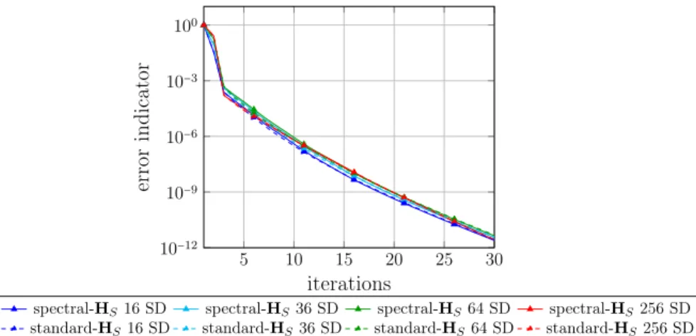
Comparison with the standard multiscale approach Henceforth, we choose the HSsearch direction in order to compare the spectral approach with the standard one. We observe in Figure 5 that the convergence rate remains similar for both procedures. Indeed, in this case where the partition resolves the heterogeneity, the spectral approach only selects the rigid body and simple deformation modes (see Figure 6) which are similar to the ones chosen in the standard approach. For the standard approach, 6 modes are defined per interface.
5 10 15 20 25 30 10−12 10−9 10−6 10−3 100 iterations error indicator
spectral-HS 16 SD spectral-HS36 SD spectral-HS64 SD spectral-HS256 SD
standard-HS16 SD standard-HS36 SD standard-HS 64 SD standard-HS256 SD
Figure 5: Weak scalability - convergence rate for the standard and spectral approaches with different number of subdomains (chessboard test-case).
(a) ˘λ3=1.042 (b) ˘λ4=1.045
(c) ˘λ5=1.046 (d) ˘λ6=1.073
7.1.2 Strong scalability
Now we study the strong scalability of the methods by keeping fixed the number of degrees of freedom and modifying the partition. For this, we start from the previous 256-subdomain case and we regroup subdomains four by four to create a new partition of 8x8 new subdomains. Therefore, these new subdo-mains are no more homogeneous, and they are composed of the two materials in a 2x2 chessboard scheme. From this new partition we apply the same procedure to obtain a new 4x4 partition. Moreover – as the subdomains are heterogeneous – we use a ˘ρ = 1.2 criterion to select the spectral modes with a maximum of 30 modes selected per subdomain. Several comments can be made:
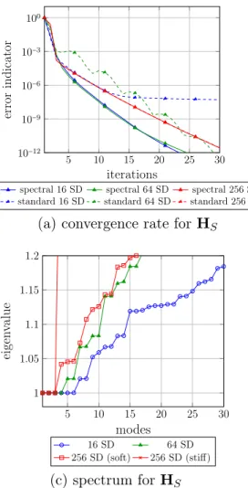
• Figure 7a-7b: with heterogeneous subdomains the standard modes are no more able to represent the heterogeneity correctly. Thus, the more heterogeneous the subdomains are, the worse the convergence rate is. In particular, the convergence of the 4x4 partition leads to stagnation whereas the 8x8 one keeps converging with a few oscillations. On the other side, the spectral approach is not really disrupted as it selects the most adapted modes automatically, however the size of the coarse problem increases with the number of modes. Moreover, when using HS we can observe that the convergence rate is extremely similar for the 4x4 and 8x8 partitions, whereas the 16x16 partition (which resolves the heterogeneity) has an inferior performance. In the case of HK, we note an improvement for the 8x8 and 16x16 respect to the 4x4 partition.
• Figure 7c-7d: it is observed that the more heterogeneous the subdomains are, the lower the first eigenvalues are. Therefore, more modes are selected. We also notice that the HK case with 16 subdomains needs more than 30 modes to satisfy the criterion ˘ρ = 1.2 and represent the whole subspace. On the other side, for the three partitions more modes are selected for HK than for HS respectively, explaining why HK leads to faster convergence for each partition.
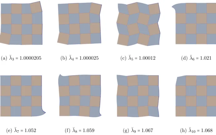
• Figure 8: the first modes for a subdomain belonging to the 4x4 partition are shown, where we can observe the role of the softer material in these deformations.
7.2 2D heterogeneous beam
In this example we show the performance of the method when the heterogeneity pattern is more complex and where the interfaces see crossing and non-crossing heterogeneity, as illustrated in Figure 9. The studied structure consists of a 2D beam with the material pattern described in Figure 10 and Table 2, submitted to a vertical flexion load on its right end. The 4-subdomain pattern is repeated 16 times to obtain 64 subdomains in total.
material 0 material 1 material 2 material 3
E0=2 MPa E1=200000MPa E2=2000MPa E3=50000MPa
ν0 =0.3 ν1=0.49 ν2=0.3 ν3=0.3
Table 2: Description of the materials (2D heterogeneous test case) 7.2.1 Study of the spectrum
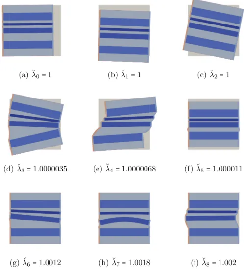
We show the spectrum of the first five subdomains in Figure 11. Excepted for the first subdomain, all others have a similar spectrum: three rigid body modes associated with the triple eigenvalue 1 followed by six modes with eigenvalues close to 1. Then, a gap is observed in the spectrum and no more modes are selected as we cut at ˘ρ = 1.05. One can remark that after the ninth first modes, the spectrum for HK is lower than for HS. We illustrate the first nine modes in Figure 12 concerning the third subdomain. Regarding the first subdomain, no rigid body modes are selected since it is a clamped subdomain. A few modes are selected, they are shown in Figure 13.
5 10 15 20 25 30 10−12 10−9 10−6 10−3 100 iterations error indicator
spectral 16 SD spectral 64 SD spectral 256 SD standard 16 SD standard 64 SD standard 256 SD
(a) convergence rate for HS
5 10 15 20 25 30 10−12 10−9 10−6 10−3 100 iterations error indicator
spectral 16 SD spectral 64 SD spectral 256 SD standard 16 SD standard 64 SD standard 256 SD
(b) convergence rate for HK
5 10 15 20 25 30 1 1.05 1.1 1.15 1.2 modes eigen v alue 16 SD 64 SD 256 SD (soft) 256 SD (stiff) (c) spectrum for HS 5 10 15 20 25 30 1 1.05 1.1 1.15 1.2 modes eigen v alue 16 SD 64 SD 256 SD (soft) 256 SD (stiff) (d) spectrum for HK Figure 7: Strong scalability - effect of the search direction HS and HK (chessboard test case). 7.2.2 Comparison with the standard multiscale approach
We contrast the convergence ratio of the spectral and classical coarse spaces. The Figure 14 shows the evolution of iterations for the two approaches and also that of the monoscale. We note a tremendous im-provement with the spectral macrospace. Moreover, the convergence ratio depends on the search direction (HS or HK).
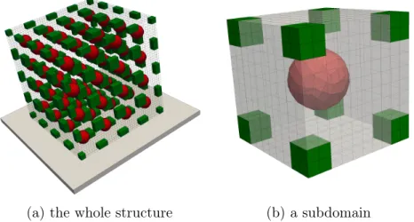
7.3 A 3D heterogeneous test case
We are here focused on a 3D cubic structure partitioned into 64 subdomains (4x4x4) with heterogeneity both inside subdomains and crossing interfaces at corners, as detailed in Figure 15. The difficulty lies in the stiffness contrast (see Table 3) between the very soft matrix – material 0 – compared to the stiff inclusions – materials 1 and 2 – which leads to a very bad conditioning, especially due to the corner inclusions. For this example, only the search direction HK is used.
material 0 material 1 material 2
E0=2 MPa E1 =200000MPa E2=200000MPa
ν0=0.3 ν1=0.3 ν2 =0.3
(a) ˘λ3 =1.0000205 (b) ˘λ4=1.000025 (c) ˘λ5=1.00012 (d) ˘λ6=1.021
(e) ˘λ7=1.052 (f) ˘λ8=1.059 (g) ˘λ9=1.067 (h) ˘λ10=1.068 Figure 8: Strong scalability - modes for an heterogeneous subdomain where the softer material is in bleu (chessboard test case).
Figure 9: Example of crossing and non-crossing interfaces.
Figure 10: Pattern of materials - material 0,material 1,material 2,material 3. 7.3.1 Homogeneous structure
Firstly, we stay in a homogeneous case where the inclusions are made out of the same material as the matrix. The purpose is to expose that rigid body modes are not enough to obtain good performance.
5 10 15 20 25 30 1 1.1 1.2 1.3 1.4 1.5 modes eigen v alue 1stSD 2ndSD 3rdSD 4thSD 5thSD
(a) spectrum for HS
5 10 15 20 25 30 1 1.1 1.2 1.3 1.4 1.5 modes eigen v alue 1stSD 2ndSD 3rdSD 4thSD 5thSD (b) spectrum for HK
Figure 11: Spectrum of the first five subdomains (2D heterogeneous test case).
(a) ˘λ0=1 (b) ˘λ1=1 (c) ˘λ2 =1
(d) ˘λ3=1.0000035 (e) ˘λ4 =1.0000068 (f) ˘λ5=1.000011
(g) ˘λ6=1.0012 (h) ˘λ7=1.0018 (i) ˘λ8=1.002
Figure 12: First nine modes of the third subdomain and their associated eigenvalues (2D heterogeneous test case).
(a) ˘λ0=1.000223 (b) ˘λ1=1.000228 (c) ˘λ2=1.00085 (d) ˘λ3=1.0022
Figure 13: First four modes of the first subdomain and their associated eigenvalues (2D heterogeneous test case). 20 40 60 80 100 10−13 10−10 10−7 10−4 10−1 iterations error indicator
monoscale HS standard HS spectral HS
monoscale HK standard HK spectral HK
Figure 14: Convergence ratio for standard and spectral approaches (2D heterogeneous test case).
(a) the whole structure (b) a subdomain
Figure 15: Geometry, material heterogeneity and partition of the 3D heterogeneous structure (material 0, material 1 andmaterial 2).
perceive some jumps, but they are not very strong. To illustrate the need of taking into account more than the very first modes, Figure 18a presents the convergence with the spectral approach for several criteria:
20 40 60 80 100 1 1.1 1.2 1.3 1.4 1.5
modes
eigen
v
alue
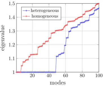
heterogeneous homogeneousFigure 16: Spectrum of an internal subdomain (3D test case).
(a) ˘λ6 =1.047 (b) ˘λ15=1.113 (c) ˘λ75=1.397
Figure 17: Some modes and their associated eigenvalues (3D homogeneous test case).
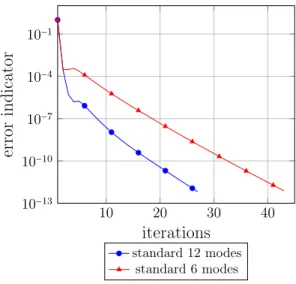
from ˘ρ = 1.1 to ˘ρ = 1.5. The main conclusion is that the first modes containing combinations of rigid body motions and other simple deformations are not sufficient. Indeed, using a criterion of ˘ρ = 1.2 the number of selected modes is doubled but it enables dividing by two the number of iterations to reach an error indicator of 10−13. Choosing a bit more modes with a criterion of ˘ρ = 1.3, the convergence at the beginning is enhanced. However, it is not necessary to select more modes, because the convergence with criteria of ˘ρ = 1.3, ˘ρ = 1.4 and ˘ρ = 1.5 remains very similar. Figure 17 shows some modes selected with different criteria. While we recognize simple deformation for the first ones, it becomes more erratic for the last ones and it remains very local. As confirmed in Figure 18a, these last modes do not really improve the convergence of the algorithm. Figure 18b compares the standard approach considering only rigid body modes and simple interface deformations. Obviously rigid body motions (6 modes) are not able to capture all the suitable information.
10 20 30 40 10−13 10−10 10−7 10−4 10−1 iterations error indicator ˘ ρ =1.1 ρ =1.2˘ ρ =1.3˘ ˘ ρ =1.4 ρ =1.5˘ (a) spectral macrospace
10 20 30 40 10−13 10−10 10−7 10−4 10−1 iterations error indicator standard 12 modes standard 6 modes (b) standard macrospace Figure 18: Convergence ratio for standard and spectral approaches (3D test case). 7.3.2 Heterogeneous structure
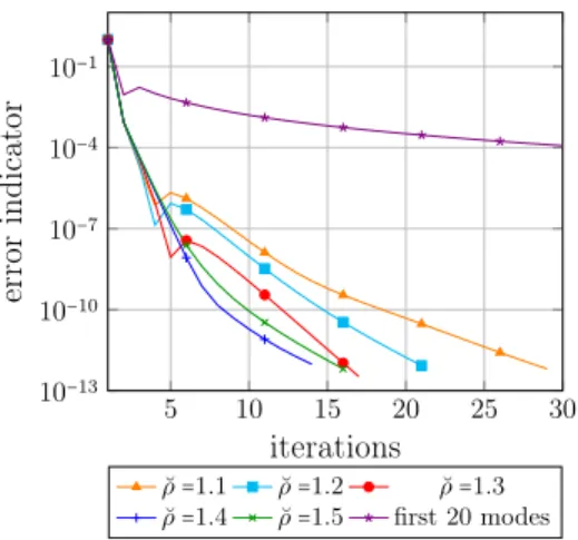
The 3D structure is here analyzed taking into account material parameters with a heterogeneity ratio of 105 (see Table 3). The spectrum of an internal subdomain is blue plotted in Figure 16. The spectrum of the homogeneous case allows to emphasize that the heterogeneous case has a very flat spectrum near to 1 for the almost 50 first modes. These first modes are rigid body motions and simple deformations of the stiff inclusions. In Figure 19 a few modes are shown.
Figure 20 exposes what occurs if the initial plateau of the spectrum (eigenvalues close to 1) is partially taken into account. In fact, only 20 modes per subdomain are not satisfying; on the contrary even the weak criterion ˘ρ = 1.1 is enough to capture the bad modes leading to a significantly improved convergence rate (fewer than 30 iterations to reach an error of 10−12). Selecting more modes by augmenting the criterion helps to improve the convergence: ˘ρ = 1.4 seems to be most adapted in this case, whereas the more stringent ˘ρ = 1.5 leads to selecting more than 100 modes per subdomains without accelerating.
(a) ˘λ6=1.00000153 (b) ˘λ30=1.0000102 (c) ˘λ48=1.115 Figure 19: Some modes and their associated eigenvalues (3D heterogeneous test case).
5 10 15 20 25 30 10−13 10−10 10−7 10−4 10−1 iterations error indicator ˘ ρ =1.1 ρ =˘ 1.2 ρ =˘ 1.3 ˘ ρ =1.4 ρ =˘ 1.5 first 20 modes
Figure 20: Convergence ratio for the spectral approach (3D heterogeneous test case).
8
Conclusion
This paper proposes an analysis of the mono and multiscale Latin method in the presence of perfect interfaces. It shows that the convergence rate of the monoscale method can be studied through local generalized eigenvalue problems. It is then possible to tell which spectral contributions are slowing down the convergence, and gather them in a “macrospace” used to constrain the resolution process. Unfortu-nately, in current state, with the multiscale Latin method only constraining the interface force field, it is not possible to warranty the bad part of the spectrum not being activated. Anyhow, even without strict bound on the convergence rate, it is possible to assess a new spectrum-motivated coarse space.
The performance of the method is illustrated of various severe heterogeneous examples. The first one consists in a weak and strong scalability study of a heterogeneous chessboard. The second test case is a 2D slender beam with various heterogeneity patterns. We observe very similar results respecto to the ones in [15] and we illustrate that the standard modes chosen for the Latin method are no more sufficient and modes adapted to the heterogeneity are required. The last test case is a 3D structure with spherical and cubic stiff inclusions into a softer material. We show that choosing more modes in addition to the rigid body modes is relevant, even in the homogeneous case, and compulsory in the heterogeneous case.
Future work will concern the full control of the spectrum of the multiscale operator, probably using more complex constraint, also applied to the displacement field.
Acknowledgment
This work was partly funded by the international project ECOS-CONICYT C17E04 between LMT and Universidad de Talca, and by the French project PIA PAMSIM.
References
[1] V. Dolean, P. Jolivet, F. Nataf, An introduction to domain decomposition methods: algorithms, theory, and parallel implementation, SIAM, 2015.
[2] J. Mandel, B. Sousedík, Adaptive selection of face coarse degrees of freedom in the BDDC and the FETI-DP iterative substructuring methods, Comput. Methods Appl. Mech. Eng. 196 (8) (2007) 1389–1399. doi:10.1016/j.cma.2006.03.010.
[3] J. Mandel, B. Sousedík, J. Šístek, Adaptive BDDC in three dimensions, Math. Comput. Simul. 82 (10) (2012) 1812–1831. arXiv:arXiv:0910.5863v2, doi:10.1016/j.matcom.2011.03.014.
[4] A. Klawonn, M. Kühn, O. Rheinbach, Adaptative coarse space for FETI-DP in three dimensions, SIAM J. SCI. Comput. 38 (5) (2016) A2880–A2911. doi:10.1137/15M10496101.
[5] A. Klawonn, P. Radtke, O. Rheinbach, A comparison of adaptive coarse spaces for iterative substruc-turing in two dimensions, Electron. Trans. Numer. Anal. 45 (2016) 75–106.
[6] C. Pechstein, C. R. Dohrmann, A unified framework for adaptive BDDC, Electronic Transactions on Numerical Analysis 46 (2017) 273–336.
[7] A. Klawonn, M. Kühn, O. Rheinbach, Adaptative FETI-DP and BDDC methods with a generalized transformation of basis for heterogeneous problems, Electronic Transactions on Numerical Analysis 49 (2018) 1–27. doi:10.1553/etna.
[8] A. Klawonn, M. Kühn, O. Rheinbach, Coarse spaces for FETI-DP and BDDC methods for het-erogeneous problems: connections of deflation and a generalized transformation-of-basis approach, Electronic Transactions on Numerical Analysis 52 (2020) 43–76. doi:10.1553/etna.
[9] M. J. Gander, Optimized Schwarz Methods, SIAM Rev. 44 (2) (2006) 699–731. doi:10.1137/ S0036142903425409.
[10] A. St-Cyr, M. J. Gander, S. J. Thomas, Optimized Multiplicative, Additive, and Restricted Additive Schwarz Preconditioning, SIAM Journal on Scientific Computing 29 (6) (2007) 2402–2425. arXiv: arXiv:1011.1669v3, doi:10.1137/060652610.
URL http://epubs.siam.org/doi/10.1137/060652610
[11] M. J. Gander, Schwarz methods over the course of time, Electronic Transactions on Numerical Anal-ysis 31 (5) (2008) 228–255. doi:10.1007/s00595-010-4443-5.
[12] M. J. Gander, Y. Xu, Optimized Schwarz methods for model problems with continuously vaiable coeffi-cients, SIAM Journal of Scientific Computing 38 (5) (2016) A2964–A2986. doi:10.1137/15M1053943. URL epubs.siam.org/doi/abs/10.1137/15M1053943
[13] M. J. Gander, T. Vanzan, Heterogeneous optimized Schwarz methods for second order elliptic PDEs, SIAM Journal of Scientific Computing 41 (4) (2019) 2329–2354. doi:10.1137/18M122114X.
URL epubs.siam.org/doi/abs/10.1137/18M122114X
[14] N. Spillane, V. Dolean, P. Hauret, F. Nataf, C. Pechstein, R. Scheichl, A robust two-level domain decomposition preconditioner for systems of PDEs, Comptes Rendus Math. 349 (23-24) (2011) 1255– 1259. doi:10.1016/j.crma.2011.10.021.
[15] N. Spillane, D. J. Rixen, Automatic spectral coarse spaces for robust finite element tearing and interconnecting and balanced domain decomposition algorithms, Int. J. Numer. Methods Eng. 95 (11) (2013) 953–990. arXiv:1010.1724, doi:10.1002/nme.4534.
[16] N. Spillane, V. Dolean, P. Hauret, F. Nataf, C. Pechstein, R. Scheichl, Abstract robust coarse spaces for systems of PDEs via generalized eigenproblems in the overlaps, Numer. Math. 126 (4) (2014) 741–770. doi:10.1007/s00211-013-0576-y.
[17] F. Nataf, Mathematical analysis of robustness of two-level domain decomposition methods with respect to inexact coarse solves, Numerische Mathematik 144 (4) (2020) 811–833. doi:10.1007/ s00211-020-01102-6.
URL https://doi.org/10.1007/s00211-020-01102-6
[18] R. Haferssas, P. Jolivet, F. Nataf, A robust coarse space for Optimized Schwarz methodsSORAS-GenEO-2, Comptes Rendus Mathematique 353 (10) (2015) 959,963. doi:10.1016/j.crma.2015.07. 014.
[19] R. Haferssas, P. Jolivet, F. Nataf, An additive schwarz method type theory for lions’s algo-rithm and a symmetrized optimized restricted additive schwarz method, SIAM Journal on Sci-entific Computing 39 (4) (2017) A1345–A1365. arXiv:https://doi.org/10.1137/16M1060066, doi:10.1137/16M1060066.
URL https://doi.org/10.1137/16M1060066
[20] R. Bridson, C. Greif, A Multipreconditioned Conjugate Gradient Algorithm, SIAM J. Matrix Anal. Appl. 27 (4) (2006) 1056–1068. doi:10.1137/040620047.
[21] P. Gosselet, D. J. Rixen, F.-X. Roux, N. Spillane, Simultaneous FETI and block FETI: Robust domain decomposition with multiple search directions, Int. J. Numer. Methods Eng. 104 (10) (2015) 905–927. arXiv:1010.1724, doi:10.1002/nme.4946.
[22] N. Spillane, An Adaptive MultiPreconditioned Conjugate Gradient Algorithm, SIAM J. Sci. Comput. 38 (3) (2016) A1896–A1918. doi:10.1137/15M1028534.
[23] C. Bovet, A. Parret-Fréaud, N. Spillane, P. Gosselet, Adaptive multipreconditioned FETI: Scalability results and robustness assessment, Comput. Struct. 193 (2017) 1–20. doi:10.1016/J.COMPSTRUC. 2017.07.010.
[24] M. C. Leistner, P. Gosselet, D. J. Rixen, Recycling of Solution Spaces in Multi-Preconditioned FETI Methods Applied to Structural Dynamics, International Journal for Numerical Methods in Engineer-ing 116 (2) (2018) 141–160. doi:10.1002/nme.5918.
[25] P. Ladevèze, Nonlinear computational structural mechanics: new approaches and non-incremental methods of calculation, Springer-Verlag New York, 1999. doi:10.1007/978-1-4612-1432-8. [26] P. Ladevèze, A. Nouy, On a multiscale computational strategy with time and space homogenization
for structural mechanics, Computer Methods in Applied Mechanics and Engineering 192 (28) (2003) 3061–3087, multiscale Computational Mechanics for Materials and Structures. doi:https://doi. org/10.1016/S0045-7825(03)00341-4.
URL http://www.sciencedirect.com/science/article/pii/S0045782503003414
[27] V. Roulet, L. Champaney, P.-A. Boucard, A parallel strategy for the multiparametric analysis of structures with large contact and friction surfaces, Advances in Engineering Software 42 (6) (2011) 347 – 358.
[28] P. A. Guidault, O. Allix, L. Champaney, C. Cornuault, A multiscale extended finite element method for crack propagation, Computer Methods in Applied Mechanics and Engineering 197 (5) (2008) 381–399.
[29] P. Kerfriden, O. Allix, P. Gosselet, A three-scale domain decomposition method for the 3D analysis of debonding in laminates, Computational Mechanics 44 (3) (2009) 343–362.
[30] V. Visseq, P. Alart, D. Dureisseix, Towards an augmented domain decomposition method for non-smooth contact dynamics models, Computational Particle Mechanics 1 (1) (2014) 15–26. doi: 10.1007/s40571-014-0005-8.
[31] A. Giacoma, D. Dureisseix, A. Gravouil, M. Rochette, Toward an optimal a priori reduced basis strategy for frictional contact problems with LATIN solver, Computer Methods in Applied Mechanics and Engineering 283 (2015) 1357–1381. doi:10.1016/j.cma.2014.09.005.
[32] P. Ladevèze, J.-C. Passieux, D. Néron, The latin multiscale computational method and the proper generalized decomposition, Computer Methods in Applied Mechanics and Engineering 199 (21) (2010) 1287 – 1296, multiscale Models and Mathematical Aspects in Solid and Fluid Mechanics. doi:https: //doi.org/10.1016/j.cma.2009.06.023.
URL http://www.sciencedirect.com/science/article/pii/S0045782509002643
[33] N. Relun, D. Néron, P. Boucard, A model reduction technique based on the pgd for elastic-viscoplastic computational analysis, Computational Mechanics 51 (2012) 83–92. doi:https://doi.org/10.1007/ s00466-012-0706-x.
[34] P. Ladevèze, O. Loiseau, D. Dureisseix, A micro–macro and parallel computational strategy for highly heterogeneous structures, International Journal for Numerical Methods in Engineering 52 (12) (2001) 121–138. doi:10.1002/nme.274.
[35] P. Oumaziz, P. Gosselet, P.-A. Boucard, S. Guinard, A non-invasive implementation of a mixed domain decomposition method for frictional contact problems, Computational Mechanics 60 (5) (2017) 797–812. doi:10.1007/s00466-017-1444-x.
[36] P. Oumaziz, P. Gosselet, P. A. Boucard, M. Abbas, A parallel noninvasive multiscale strategy for a mixed domain decomposition method with frictional contact, Int. J. Numer. Methods Eng. 115 (8) (2018) 893–912. doi:10.1002/nme.5830.
[37] E. R. D, code-aster.
URL www.code-aster.org
[38] D. Rixen, C. Farhat, A simple and efficient extension of a class of substructure based preconditioners to heterogeneous structural mechanics problems, Internat. J. Num. Meth. Engin. 44 (4) (1999) 489– 516. doi:10.1002/(SICI)1097-0207(19990210)44:4<489::AID-NME514>3.0.CO;2-Z.
[39] A. Klawonn, O. B. Widlund, FETI and Neumann-Neumann iterative substructuring methods: Connections and new results, Commun. Pure Appl. Math. 54 (1) (2001) 57–90. doi:10.1002/ 1097-0312(200101)54:1<57::AID-CPA3>3.0.CO;2-D.
[40] P. Gosselet, C. Rey, D. Rixen, On the initial estimate of onterface forces in FETI methods, Computer Methods in Applied Mechanics and Engineering 192 (2003) 2749–2764. doi:10.1016/ S0045-7825(03)00288-3.
[41] K. Saavedra, O. Allix, P. Gosselet, J. Hinojosa, A.-E. Viard, An enhanced nonlinear multi-scale strategy for the simulation of buckling and delamination on 3D composite plates, Computer Methods in Applied Mechanics and Engineering 317 (2017) 952–969. doi:10.1016/j.cma.2017.01.015. URL http://dx.doi.org/10.1016/j.cma.2017.01.015