HAL Id: hal-00817201
https://hal-pjse.archives-ouvertes.fr/hal-00817201v2
Preprint submitted on 15 Oct 2013
HAL is a multi-disciplinary open access
archive for the deposit and dissemination of sci-entific research documents, whether they are pub-lished or not. The documents may come from teaching and research institutions in France or abroad, or from public or private research centers.
L’archive ouverte pluridisciplinaire HAL, est destinée au dépôt et à la diffusion de documents scientifiques de niveau recherche, publiés ou non, émanant des établissements d’enseignement et de recherche français ou étrangers, des laboratoires publics ou privés.
Learning in a Black Box
Heinrich H. Nax, Maxwell N. Burton-Chellew, Stuart A. West, H. Peyton
Young
To cite this version:
Heinrich H. Nax, Maxwell N. Burton-Chellew, Stuart A. West, H. Peyton Young. Learning in a Black Box. 2013. �hal-00817201v2�
WORKING PAPER N° 2013 – 10
Learning in a Black Box
Heinrich H. Nax Maxwell N. Burton-Chellew Stuart A. West H. Peyton Young JEL Codes : C70, C73, C91, D83, H41
Keywords: Learning; Information; Public goods games
P
ARIS-
JOURDANS
CIENCESE
CONOMIQUES48, BD JOURDAN – E.N.S. – 75014 PARIS TÉL. : 33(0) 1 43 13 63 00 – FAX : 33 (0) 1 43 13 63 10
Learning in a Black Box
∗
H.H. Nax
†, M.N. Burton-Chellew
‡, S.A. West
§, H.P. Young
¶First version: April 18, 2013
This version: September 30, 2013
∗We thank Margherita Comola for help at an early stage of the project and Johannes Abeler, Richard Bradley, Fabrice Etil´e, Philippe Jehiel, Thierry Verdier, Vince Crawford, Colin Camerer, Guillaume Hollard, Muriel Niederle, Edoardo Gallo, Amnon Rapoport, Guillaume Fr´echette and participants of the Economics and Psychology seminar at MSE Paris, the Choice Group at LSE and the 24th Game Theory Workshop at Stony Brook for helpful discussions, suggestions and comments. Correspondence to: H. H. Nax, 48 Boulevard Jourdan, Bureau A201, Paris School of Economics, 75014 Paris, France.
†Heinrich H. Nax, Paris School of Economics, ´Ecole Normale Sup´erieure. Nax’s research was in part supported by the Office of Naval Research grant N00014-09-1-0751 and under project NET of the Agence Nationale de Recherche.
‡Maxwell N. Burton-Chellew, Nuffield College, Oxford & Department of Zoology, University of Oxford (The Tinbergen Building S Parks Rd, Oxford OX1 3PS, United Kingdom).
§Stuart A. West, Department of Zoology, University of Oxford (The Tinbergen Building S Parks Rd, Oxford OX1 3PS, United Kingdom). Burton-Chellew and West’s research was supported by the European Research Council.
¶H. Peyton Young, Department of Economics, University of Oxford (Nuffield College, New Rd, Oxford OX1 1NF, United Kingdom). Young’s research was supported in part by the Office of Naval Research grant N00014-09-1-0751.
Abstract
Many interactive environments can be represented as games, but they are so large and complex that individual players are in the dark about others’ actions and the payoff structure. This paper analyzes learning behavior in such ‘black box’ environments, where players’ only source of information is their own history of actions taken and payoffs received. Specifically we study voluntary contributions games. We identify two robust features of the players’ learning dynamics: search volatility and trend-following. These features are clearly present when players have no information about the game; but also when players have full information. Convergence to Nash equilibrium occurs at about the same rate in both situations.
JEL classifications: C70, C73, C91, D83, H41
Keywords: learning, information, public goods games
1
Introduction
Many interactive environments can be represented as games, but they are so complex and involve so many individuals that for all practical purposes the game itself is unknown to the players themselves. Examples include bidding in on-line markets, threading one’s way through urban traffic, or participating in a group effort where the actions of the other members of the group are difficult to observe (guerrilla warfare, neighborhood watch programs, tax evasion). In each of these cases a given individual will have only the haziest idea of what the other players are doing but their payoffs are strongly influenced by the actions of the others. How do individuals learn in such environments and under what circumstances does their learning behavior lead to equilibrium?
In this paper we investigate these questions in a laboratory environment where the un-derlying game has the structure of a public goods game. Players take actions and receive payoffs that depend on others’ actions, but (in the baseline case) they have no informa-tion about the others and they do not know what the overall structure of the game is. This distinguishes our experimental setup from other “low-information” setups such as Rapoport et al. (2002) and Weber (2003) who provide information about the structure of the game but withhold information about the distribution of players’ types and the outcome of play, or Friedman et al. (2012) who withhold information about the payoff structure of the game but provide information about other players’ actions and payoffs. The closest “low-information” set-up to ours is that of Bayer et al. (2013) who also implement experiments without information about the structure of the game and about
other players. However, their set-up purposefully induces a “confusion” element that the game structure itself may also change. In our setup, the structure of the game, although it is unknown to the agents, remains fixed and agents know that. Perhaps the closest antecedent of our ‘black box’ treatments are repeated two-by-two zero sum games used to test the early Markov learning models by Suppes & Atkinson (1959).1
As the game proceeds, all agents know is the amount that they themselves contributed and the payoff they received as a result. Learning in such an explicitly repated game environment is said to be completely uncoupled (Foster & Young, 2006; Young, 2009; see also Hart & Mas-Colell, 2003, 2006;). In this setting many of the standard learning rules in the empirical literature, such as experience-weighted attraction, k-level reasoning, and imitation, do not apply because these rules use the actions of the other players as inputs (Bj¨ornerstedt & Weibull, 1993; Stahl & Wilson, 1995; Nagel, 1995; Ho et al., 1998; Camerer & Ho, 1999; Costa-Gomes et al., 2001; Costa-Gomes & Crawford, 2006).2
Nevertheless our experiments show that learning ‘inside the box’ can and does take place.3 The learning process exhibits certain distinctive patterns that have been identified in other settings. Two especially noteworthy features are the following:
Search volatility. A decrease in a player’s realized payoff triggers greater variance in his choice of action next period, whereas an increase in his realized payoff results in lower variance next period.
Trend-following. If a higher contribution leads to a higher payoff this period, the player will tend to raise his contribution next period, whereas if a higher contribution leads to a lower payoff this period, he will tend to reduce his contribution next period. Similarly, if a lower contribution leads to a higher payoff the player will tend to lower his contribution, whereas if a lower contribution leads to a lower payoff he will tend to increase his contribution next period.
Learning rules with high and low search volatility have been proposed in a variety of set-tings, including biology (Thuijsman et al., 1995), organizational learning (March, 1991),
1Note that subjects in that setting have only two strategies and were explicitly ‘fooled’ not to think that they were playing a game. The observed learning in this setting follows reinforcement.
2Indeed most impulse-based learning models (see Crawford, 2013) except for reinforcement learning (Erev & Roth, 1998) are thus excluded. We also note that social preferences cannot enter into subjects’ behavior because they cannot compare their own payoffs with others’ payoffs. Thus the black box environment eliminates some of the explanations that have been advanced for behavior in public goods games (Fehr & Schmidt, 1999; Fehr & Gachter, 2000, 2002; Fehr & Camerer, 2007).
3Oechssler & Schipper (2003) show that, in the context of 2x2 games, players can learn to identify the other player’s payoff structure on the basis of their own payoffs and information about other’s actions. In our set-up players may or may not learn the game, but even without information about the relationship between their own and others’ payoffs they do learn to play Nash equilibrium. See Erev & Haruvy (2013) for a recent survey of equilibrium learning.
computer science (Eiben & Schippers, 1998), and psychology (Coates, 2012). (In com-puter science and organization theory this type of learning is known as ‘exploration versus exploitation’, ‘win-stay-lose-shift’ or ‘fast and slow’ learning.) Search volatility is also a crucial feature of rules that have recently been proposed in the theoretical literature; in particular there is a family of such rules that lead to Nash equilibrium in generic n-person games (Foster & Young, 2006; Germano & Lugosi, 2007; Marden et al., 2009; Young, 2009; Pradelski & Young, 2012). To our knowledge, despite systematic differences in behavior following positive and negative feedback being noted (e.g. Ding & Nicklisch, 2013), our model is the first experimental text of an explicit learning model with such this feature.
Trend-following also has antecedents in the experimental literature, where it is sometimes called directional learning (Selten & Stoecker, 1986; Selten & Buchta, 1998).4 Directional
learning describes behavioral dynamics based on local adjustments of strategy and aspi-ration (Sauermann & Selten, 1962; Cross, 1983). The underlying behavioral components are illustrated in a bargaining game: if a higher demand results in a higher realized payoff the agent increases his demand, whereas a decrease in realized payoff leads to a demand decrease (Tietz & Weber, 1972; Roth & Erev, 1995). Other experiments such as Erev & Roth (1998) and Erev & Rapoport (1998) corroborate these bargaining findings and Nash equilibrium is learned based on reinforcement dynamics in various settings. Recent the-oretical generalization’s of directional learning when strategies are unidimensional have been proposed by Laslier & Walliser (2011). Bayer et al. (2013) recover a directional learning model in their learning condition even if the structure of the game potentially changes.
In this paper we show that these two patterns help explain the behavior of subjects who are learning in a ‘black box’ environment. Moreover, despite the lack of information and the simplicity of the adjustment rules, the behavior of the group approaches Nash equilibrium and does so at approximately the same rate as in the situation where subjects have full information (Burton-Chellew & West, 2012). As we shall see, this is true both when free riding is the dominant strategy, and also when full contribution is the dominant strategy. We conclude that even when subjects have virtually no information about the game, learning follows certain distinctive patterns that have been documented in a wide variety of learning environments. In public goods games this behavior leads to Nash equilibrium at a rate that is very similar to learning under full information. Moreover, search volatility turns out to be a robust behavioral component even when more information becomes available and when players gain experience.
The paper is structured as follows. In section 2 we describe the experimental set-up in detail. In section 3 we present the empirical findings together with statistical tests of significance. We conclude in section 4. An appendix contains experimental instructions and supplementary regression tables.
2
Experimental set-up
Participants were recruited from a subject pool that had not previously been involved in public goods experiments.5 The subjects were not limited to university students,
but included different age groups with diverse educational backgrounds.6 Each subject
played four separate contribution games, where each game was repeated twenty times with randomly allocated subgroups. The twenty-fold repetition of a given game will be called a ‘phase’ of the experiment. This yields a total of 236 games and 18,880 observations. During sixteen separate sessions in groups of sixteen or twelve, subjects play the four phases in a row.
Games differ with respect to two rates of return (‘low’ and ‘high’) such that either ‘free-riding’ or ‘fully contributing’ is the dominant strategy. Treatments differ with respect to the information that is revealed to the agents (‘black box’, ‘standard’ and ‘enhanced’). Every player plays both black box games, and either the two standard or enhanced information games. Either two black box games are played first, or two games of one of the other two treatments.7 The two first phases constitute stage one, the second two constitute stage two. Each possible information order is played in four separate sessions, each of which with a different order of the two rates of return.8
In this section, we shall describe the underlying stage game, the structure of each repeated game, and the different information treatments.
5The subjects were recruited through ORSEE (Online Recruiting System for Economic Experiments; Greiner, 2004) with this request specifically made.
6The experiment was programmed and conducted with the software z-Tree (Fischbacher, 2007). All experiments were conducted at the Centre for Experimental Social Sciences (CESS) at Nuffield College, University of Oxford.
7Of the 18,880 observations, 9,440 are black box, 4,640 are standard, and 4,800 are enhanced. 8This yields sixteen different scenarios each played in one of the sessions given by the possible orders and permutations; four (combinations) times four (orders) equals sixteen (sessions).
2.1
Linear public goods game
Consider the following linear public goods game. Every player i in population N = {1, 2, ..., n} makes a nonnegative, real-numbered contribution, ai, from a finite budget
B ∈ N+. Given a resulting vector of all players’ contributions, a = {a1, a2, ..., an}, for
some rate of return, e ≥ 1, the public good is provided, R(a) = eP
i∈Nai, and split
equally amongst the players.9 Given others’ contributions a
−i, player i’s contribution ai
therefore results in a payoff of φi = e n X i∈N ai+ (B − ai),
where en is the marginal rate of return. Write φ for the payoff vector {φ1, ..., φn}.
Nash equilibria. Depending on whether the rate of return is low (e < n) or high (e > n), individual contribution of either zero (free-riding) or B (fully contributing) is the strictly dominant strategy for all players; the respective Nash equilibrium results in either nonprovision or full provision of the public good.10
2.2
Repeated game
In any session, the same population S (with |S| = 12 or 16) plays four phases. Each phase is a twenty-times repeated, symmetric public goods game. In each period t of each game, players in S are randomly matched to groups of four to play the stage game.11 The
budget every period is a new B = 40 to every player of which he can invest any amount, but he cannot invest money carried over from previous rounds. The rate of return is either low (e = 1.6) or high (e = 6.4) throughout the game.12 Write N4t for any of the four-player groups matched at time t, and ρt4 for the partition of S into such groups. Given at, ρt
4, N4t, in any period t such that i ∈ N4t∈ ρt4, each i receives
φi = X t=1,...,20 φti = X t=1,...,20 [e/4X j∈Nt 4 atj+ (40 − ati)].
For every i, φi represents a real monetary value that is paid after the game.13
9If e < 1, R(a) is a public bad.
10When e = n, any contribution is a best reply to any level of contribution by the others, hence any level of provision is supported by at least one pure-strategy Nash equilibrium.
11This follows the random ‘stranger’ rematching of Andreoni (1988).
12The Nash equilibrium payoffs of the stage games are 40 when e = 1.6, and 256 when e = 6.4. 13Hundred coins are worth £0.15 to pay £19.2 maximal individual earnings from the whole experiment.
2.3
Information treatments
Before the first game begins, each player is told that two separate experiments will be played. (From the analyst’s point of view the experiment consists of both of these taken together.) At no point before, during, or in between the separate phases of the exper-iment are players allowed to communicate. Depending on which treatment is played, the following information is revealed at the start of each stage when a new treatment begins.
All treatments. Two separate twenty-times repeated stage games are played. In each, the underlying stage game is unchanged for 20 periods. Each player receives 40 monetary units each period of which he can invest any amount. Moreover, after investments are made, each player gets a nonnegative return each period which, at the end of each game, he receives together with his uninvested money according to a known exchange rate.
Black box. No information about the structure of the game, or about other players’ actions or payoffs is revealed. Throughout the game players only know their own contribution and payoffs.
Standard. The rules of the game are revealed including production of the public good, rate of return, and how groups in the session form to play each stage game. In addition, at the end of each period, players receive a summary of the relevant contributions in their previous-period group; without knowing who these players are and what payoffs they receive.14
Enhanced. In addition to the information available in the standard treatment, players learn about the other group members’ previous-period payoffs.
Our main treatment is black box. Indeed, all our results concerning the learning rules are based on black box data from sessions when black box is played first, in which case subjects really have no knowledge of the structure of the game. For this reason, we also required the recruiting system (ORSEE) to select only ‘first timers’ in public-goods experiments. (See Appendix A for full black box instructions and Appendix B for the output screens displayed during the experiment for each treatment.)
14This follows the standard information treatment design as in Fehr & Gachter (2002) and random ‘stranger’ rematching of subjects as introduced by Andreoni (1988).
3
Findings
First, we analyze the black box data when players have no prior experience playing public goods games in our experiments (or in other prior experiments). In this ‘black box’ treatment, subjects have no knowledge of the structure of the game and receive no information about others’ actions or payoffs.
3.1
Black box
In this section, we analyze the black box treatments when played before the standard or enhanced treatments. Subjects were chosen only if they had not previously participated in any public goods related experiment prior to ours.15 There were eight such sessions and
4,960 observations. By choosing these sessions, we ensure that players not only have no explicit knowledge of the game structure and no information about others, but also have no “experience” of related laboratory experiments that they could use to make structural inferences. Unless stated otherwise, “significance” refers to a 95% confidence interval (5% significance) when rejecting the null and to a 90% confidence interval (10% significance) when the null cannot be rejected.
3.1.1 Contributions
For both rates of return independent of whether played first or second (phase one or two), the mean initial contribution lies between one third and half the budget. The mean is 15.3 in the games with e = 1.6, and 13.9 in the games with e = 6.4. Using period-specific Mann-Whitney tests, we cannot reject the null of equal contributions for games with different rates of return and for phase one versus phase two, that is, similar observations are made in all games (with different rates of return) played in all initial black box treatment games. This is evidence of “restart effects” (observed throughout the literature).16 The period-two adjustments to the initial contribution have means close to zero.17 Notably, a large part of these contributions lie at 0, 10, 20, 30, 40, with several contributions made also in the range from 1 to 9; contributions at other numerical values are rare.18 Using period-specific Mann-Whitney tests, we cannot reject the null of equal
contributions for different rates of return for periods 1 through to period 3.
15We used ORSEE to recruit our subjects with this ‘first timer’ characteristic. In Section 4, we will test for experience and information effects by comparison with the rest of the data.
16See Andreoni, 1988; Croson, 1996; Cookson, 2000; Camerer, 2003. 17Means are 0.4 when e = 1.6 and 1.6 when e = 6.4.
Figure 1: Initial contributions (phases 1,2). 15 20 25 30 F re q u e n cy Period 1, e=1.6 0 5 10 0123456789 10 11 12 13 14 15 16 17 18 19 20 21 22 23 24 25 26 27 28 29 30 31 32 33 34 35 36 37 38 39 40 F re q u e n cy Contributions 15 20 25 30 F re q u e n cy Period 1, e=6.4 0 5 10 0123456789 10 11 12 13 14 15 16 17 18 19 20 21 22 23 24 25 26 27 28 29 30 31 32 33 34 35 36 37 38 39 40 F re q u e n cy Contributions 8 10 12 14 16 18 20 F re q u e n cy Period 2, e=1.6 0 2 4 6 8 0123456789 10 11 12 13 14 15 16 17 18 19 20 21 22 23 24 25 26 27 28 29 30 31 32 33 34 35 36 37 38 39 40 F re q u e n cy Contributions 10 15 20 25 F re que nc y Period 2, e=6.4 0 5 10 0123456789 10 11 12 13 14 15 16 17 18 19 20 21 22 23 24 25 26 27 28 29 30 31 32 33 34 35 36 37 38 39 40 F re q ue n cy Contributions
Initial contributions often lie at 0, 10, 20, 30, 40, with several contributions made also in the range from 1 to 9; contributions at other numerical values are rare.
(Figure 1 illustrates. See Appendix C, tables 4 and 5 for details.)
In the early periods of black box treatments, this is the behavior one would expect and it is consistent with hundreds of previous experiments on public goods.19 Since players
have no knowledge of the differences in the game structures, they initially make ran-dom contributions and play different games in much the same way. Note that players initially contribute less than half of their budget, another observation consistent with previous experimental results. A possible explanation for this is ambiguity aversion (Ep-stein, 1999).20 At the beginning of the game, players cannot judge their initial payoffs
to be particularly “good” or “bad”, and therefore have no comparison concerning the performance (“success” vs. “failure”) of different strategies. One would consequently not expect an obvious direction for the initial-period adjustments, and indeed they are similarly random until period 3 for the different rates of return.
19As surveyed, for example, in Chaudhuri, 2011.
20In Fehr & Schmidt, 1999, for example, mean contributions are ca. 40 percent of the budget; this would mean ca. 16 in our experiment.
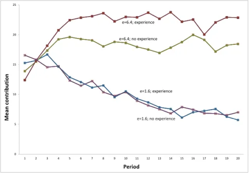
Figure 2: Mean black box play (phases 1,2). 25 e=6.4 20 15 10 Me a n c o n t r ib u t io n e=1.6 10 Me a n c o n t r ib u t io n 5 Me a n c o n t r ib u t io n 0 1 2 3 4 5 6 7 8 9 10 11 12 13 14 15 16 17 18 19 20 Period Period
Contributions deteriorate in the free-riding game. This trend is accentuated compared to the full-contribution games which display a weak positive trend.
(Figure 2 illustrates.)
If players were not to learn at all, one would expect similar behavior throughout the games. Using period-specific Mann-Whitney tests, however, we reject the null of equal contributions for different rates of return in all periods after period 3. Moreover, play evolves following distinctly different patterns: the contributions towards the end of the game are closer to the respective stage game Nash equilibrium.21 Simple linear regressions
of contributions on a time trend (controlling for phase and group) reveal a trend of -0.6 when e = 1.6 (significant at 1%), and of +0.1 when e = 6.4 (significant at 10%). Note the trend is accentuated in the games with e = 1.6.22 When e = 6.4, the mean contribution never exceeds twenty and thus remains more than “halfway” from the Nash contribution. Again, players’ ambiguity aversion may explain this phenomenon.23
21Means are 5.7 when e = 1.6 and 18.5 when e = 6.4.
22This pattern is consistent with previous experiments as, for example, noted in Ledyard, 1995. Note our contributions decline more sharply than in Bayer et al. (2013), possibly indicating a “within-game restart effect” in their experiments since players are lead to believe that underlying stage games are changing.
23A contribution decrease represents less ambiguity and is, ceteris paribus, preferred by ambiguity-averse agents, a contribution increase results in more ambiguity (Schmeidler, 1989).
Figure 3: Final contributions. 20 25 30 35 40 45 50 F re q u e n cy Period 20, e=1.6 0 5 10 15 20 0123456789 10 11 12 13 14 15 16 17 18 19 20 21 22 23 24 25 26 27 28 29 30 31 32 33 34 35 36 37 38 39 40 F re q u e n cy Contributions 15 20 25 30 F re q u e n cy Period 20, e=6.4 0 5 10 0123456789 10 11 12 13 14 15 16 17 18 19 20 21 22 23 24 25 26 27 28 29 30 31 32 33 34 35 36 37 38 39 40 F re q u e n cy Contributions
Final contributions amass close to zero in the free-riding game, and split between contri-butions close to zero and 40 for the full-contribution game.
(Figure 3 illustrates. See Appendix C, table 6 for details.)
To summarize our observations regarding aggregate contributions in free-riding games, we reconfirm the standard findings from the literature regarding initial contributions, restart effects and contribution deterioration. Moreover, we note that in games where full contribution is a Nash equilibrium, the observed trends to Nash equilibrium are substantially weaker. Higher contributions seem harder to learn.
3.1.2 Difference in variation
Adjustment. The adjustment of a player i in period t is at+1i − at i.
Success versus failure. A player i experiences success in period t + 1 if his realized payoff does not go down (φt+1i ≥ φt
i); otherwise he experiences failure.
Based on a Levene’s test (robust variance), the hypothesis of equal variances of adjust-ments following success versus failure is rejected with 99% confidence.24 Furthermore, we regress absolute adjustments on success versus failure controlling for phase, period, individual, group, and two lags of contributions and payoffs. We obtain a significantly (with 99% confidence) smaller coefficient of adjustment following success (by -1.2) than after failure. The phase dummies are not significant. None of the period dummies is significant after period 3. The two previous contributions are significant. The previous-period payoffs are significant, those lagged two previous-periods are not significant. We conclude that players’ adjustments after successful contributions have a smaller variation than ad-justments after unsuccessful contributions. As discussed in sections 1 and 2 of this paper,
Table 1: Adjustments after success and failure (phases 1,2).
statistic success failure
variance 123.9 188.5
mean +0.8 -1.2
SEARCH: the variance after success is lower than after failure; the average adjustments are close to zero.
the phenomenon of “different adjustments following success versus failure” is a feature of “search” in several recent learning models.25 Subsequently, we shall refer to this feature
as SEARCH.
(Table 1 summarizes. See also Appendix C, table 7 for details.)
3.1.3 Directional learning
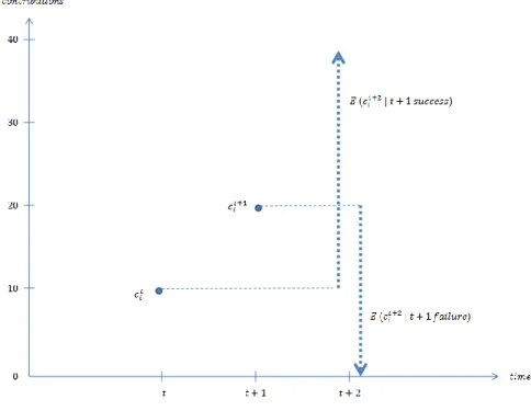
Our games have the following structure, of which subjects in the black box are unaware. First, despite knowing that they can make any contribution in the range from 0 to 40, subjects do not know that the Nash equilibrium lies at either end. Second, an individual’s payoff rises with the contributions of the other players but may rise or fall with his own adjustment depending on the game’s underlying rate of return. Importantly, in varying his own contribution, the individual agent is unable to distinguish between a self-induced success versus failure, and one that is caused by others: in the interplay with others, incremental adjustments in either direction may lead to higher or lower payoffs.26
The structure of the action space calls for a directional learning model (Selten & Stoecker, 1986; Selten & Buchta, 1998) based on success-versus-failure stimuli. Given period t, a player i may increase or decrease his contribution relative to his contribution in the previous period. As a result, he experiences either success or failure. Table 2 shows the model of directional adjustments that we propose and shall subsequently refer to as TREND.
To test the TREND hypothesis, given two subsequent payoffs, φt+1i and φt
i, we regress
adjustments relative to two lags of contributions (ct+2i − ct
i) and adjustments relative to
25See Young, 2009; Marden et al., 2011; Pradelski & Young, 2012.
26The effects that a player’s own actions and those of others have on one’s own payoff are important features in Young, 2009; Marden et al., 2011; Pradelski & Young, 2012.
Table 2: TREND hypothesis.
given success in period t given failure in period t
Player i in period t + 1 (φt i ≥ φ t−1 i ) (φti < φ t−1 i )
given an increase in period t increases contribution decreases contribution
(at i > a
t−1
i ) with respect to period t − 1 with respect to period t
given a decrease in period t decreases contribution increases contribution
(at i < a
t−1
i ) with respect to period t − 1 with respect to period t
previous contributions (ct+2i − ct−1
i ) separately.
After success (φt+1i ≥ φt
i), we obtain significant coefficients in line with the TREND
hypothesis for adjustments relative to two lags of contributions (ct+2i − ct
i): we observe a
significant increase with respect to contributions two periods ago (+7.1; significant at 1%) following an increase; and we observe a significant decrease with respect to contributions two periods ago (-12.5; significant at 1%) following a decrease. The previous contribution has a negative effect (-0.2; significant at 1%). All other coefficients are insignificant as in the failure case. Trend following after success therefore summarizes as follows:
• If an increase is a success in the current period, the average next-period adjustment relative to the previous period –net of negative level effects– is another increase. Similarly, if a decrease is a success in the current period, the average next-period adjustment relative to the previous period –net of negative level effects– is another decrease.
After failure (φt+1i < φt
i), we obtain significant coefficients in line with the TREND
hypothesis for adjustments relative to previous contributions (ct+1i − ct
i): we observe
significant coefficients for decrease with respect to the previous-period contribution (-3.4; significant at 1%) following an increase; and we observe significant increase with respect to the previous-period contribution (+2.2; significant at 1%) following a decrease. None of the phase or group dummies is significant. None of the period dummies after period 4 is significant. Past payoffs have significant but marginal (less than 0.05) effects. The previous contribution has a negative effect (-0.6; significant at 1%). Trend reversal after failure therefore summarizes as follows:
• If an increase is a failure in the current period, the average next-period adjustment relative to the current period –net of negative level effects– is a decrease instead.
Figure 4: TREND without level effect.
TREND without level effects: success versus failure leaves an intermediate range over which predictions are ambiguous.
Similarly, if a decrease is a failure in the current period, the average next-period adjustment relative to the current period –net of negative level effects– is an increase instead.
Based on TREND, given two previous contributions and a success versus failure stimulus, the location of the expected next-period contribution is known relative to the relevant previous contribution, but, given the same two previous contributions, the relative loca-tion of the contribuloca-tion depending on success versus failure is unknown. This is because TREND implies adjustment tendencies only with respect to the current period after fail-ure, and with respects to the previous period after success. It is unclear where, given both current and previous contributions, the next-period contribution will lie after either success or failure is experienced.
(Figure 4 illustrates. See also Appendix C, table 8 for details.)
We shall illustrate this point with an example as illustrated in Figure 4, if an agent contributes 10 in one period and 20 in the next, on average he contributes at least 10 if 20 was a success, and less than 20 if 20 was a failure. The following (stronger)
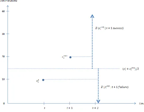
Figure 5: Average adjustment hypothesis (Bayer et al., 2013).
The average adjustment hypothesis ignores level effects and places further structure on TREND, making predictions over the intermediate range where TREND remained am-biguous.
hypothesis has been considered (Bayer et al., 2013): given two previous contributions, the next contribution is, in expectation, closer to the contribution which resulted in a higher payoff. If the stimulus is trend-neutral, the expectation lies exactly at the average. As illustrated in Figure 5, if an agent contributes 10 in one period and 20 in the next, on average he contributes at least 15 if 20 was a success, and less than 15 if 20 was a failure.
(Figure 5 illustrates. See Appendix C, table 9 for details.)
We regress contribution adjustments on the four trends controlling for phase, period, individual, group, two payoff lags, previous contribution. This yields the following ef-fects:
given at i and a
t+1
i of some individual i, the net average adjustments, controlling for level
E(at+2i ; at+1i , ati) −ati+a t−1 i 2 = φ t i ≥ φ t−1 i φti < φ t−1 i at i > a t−1 i +3.6 ∗∗ +0.3◦◦ ati < at−1i −6.5∗∗ −1.9∗◦
∗∗: significant at 1%, consistent with the average hypothesis. ◦◦: insignificant, inconsistent with the average hypothesis. ∗◦: significant at 1%, inconsistent with the average hypothesis.
Note that the adjustments following success point in the “right” direction (following success) and are significant. The adjustments following failure point in the “wrong” direction (following failure) and are significant in case of decrease. As before, the previous contribution has a significant negative effect of -0.4 (with 99% confidence). Previous profits have a marginal but significant effect. If we drop the two payoff lags and the previous contribution from the regression (since they are not included in the average adjustment model), we improve in terms of the model’s predictions but not regarding all aspects:
given at
i and a t+1
i of some individual i, the gross average adjustments, not controlling
for level effects, are
E(at+2i ; at+1i , at i) − at i+a t−1 i 2 = φ t i ≥ φ t−1 i φti < φ t−1 i ati > at−1i +1.4∗ −3.3∗∗ at i < a t−1 i −5.4 ∗∗ −0.9◦◦ ∗
: significant at 5%, consistent with the average hypothesis.
∗∗: significant at 1%, consistent with the average hypothesis. ◦◦: insignificant, inconsistent with the average hypothesis.
contribution level effects. Ceteris paribus, a higher previous-period contribution leads to a negative adjustment. Depending on trend stimulus (success or failure), success trends are followed with respect to the contribution two periods ago, failure trends are reversed with respect to the previous contribution. The size of the adjustments relative to the previous two-period average is ambiguous and depends on the level of the previous-period contribution as well as the spread of the two previous contributions. A learning model assuming average adjustments without level effects gives consistent predictions in the success and increase directions; given a decrease-failure, however, it may lead to wrong predictions. It is worth noting that in the context where the average adjustment rule was originally formulated (Bayer et al., 2013), the problematic decrease-failure trends are relatively rare because only games where free-riding is Nash are played. The most common failure in those games comes from contributing more, not less.27
3.2
Experience effects
In this section, we analyze the whole black box data including sixteen sessions and 9,440 observations. In 4,480 observations, individuals have “experience” in the sense that they play the black box games in the second stage having previously played a non-black box treatment in the first stage where they received information about the game structure in the form of detailed game instructions and about other players’ past actions (and payoffs). Even though subjects are explicitly told that a separate experiment is started after the first stage of the experiment, there is evidence that experience matters. This can be explained by subjects linking the black box game to the previous voluntary contributions games which seems reasonable given that payoffs will be similar and the action space is the same.
(Figure 6 illustrates. See Appendix C, table 10 for details.)
First, we test for distributional differences in contributions using period-specific Mann-Whitney tests for the two rates of return separately.28 The following observations are
made. In the initial period, restart effects are noted as previously. For both rates of return separately, the null hypothesis of equal contributions dependent on experience versus no experience cannot be rejected. Furthermore, there is no significant difference in between the two rates of return which is natural since players have no basis to distinguish between
27Conversely, in the games where fully contributing is Nash, decreases are the more common failures. 28Appendix C also contains regressions that cluster on individuals for the initial period and all other periods separately. The basic message being that there are significant differences if e = 6.4 but no significant differences in the initial periods or if e = 1.6
Figure 6: Mean black box play (phases 1,2 versus 3,4). e=6.4; experience 25 e=6.4; experience e=6.4; no experience 20 15 e=1.6; experience 10 Me a n c o n t r ib u t io n e=1.6; no experience 10 Me a n c o n t r ib u t io n e=1.6; no experience 5 Me a n c o n t r ib u t io n 0 1 2 3 4 5 6 7 8 9 10 11 12 13 14 15 16 17 18 19 20 Period Period
Experience plays no visible role in the free-riding games. Experience has a positive effect in the full-contribution games.
them.29 If e = 6.4, the null hypothesis of equal contributions dependent on experience versus no experience can be rejected with 90% confidence after period 5 except for periods 16 and 17. If e = 1.6, it cannot be rejected in any period.
Second, we compare the linear time trends of contributions (Appendix C, table 11 contains the details). Simple linear regressions controlling for phase and group reveal a similar trend as before if e = 1.6 (-0.5; significant at 1%) but a stronger drift e = 6.4 (+0.3; significant at 1%). Previously the respective trends were -0.6 (99%) and +0.1 (90%). Indeed, the time trends are not significant from each other if e = 1.6, but the time trend is significantly larger with experience than without experience if e = 6.4.30 Hence the contributions in games with high rates of return improve faster with experience, but there is no significant difference in play of games with low rates or return.
Finally, we perform the linear regressions with respect to SEARCH (absolute size of ad-justments) and TREND (directional adad-justments) from the previous section controlling for the same effects and adding experience dummies for both rates of return. We obtain
29The initial contributions for both rates of return lie between 14 and 15 in all four phases of the experiment.
the following results. The absolute size of adjustments (SEARCH) is smaller after the initial two periods (all period dummies after period 3 are negative and significant), and decreasing with experience. As before, the previous contribution is a positive and signif-icant factor. Payoff level effects are signifsignif-icant but marginal. All other effects (including phase dummies) are not significant. With respect to directional adjustments (TREND), experience leads to larger contributions but the direction of adjustments is unchanged. As before, the level of previous contributions is a negative and significant factor. All period dummies after period 4 are negative. All other effects are as before.
We conclude that experience has two main effects. On the one hand, experience decreases the SEARCH effect but preserves its sign. On the other hand, experience leads to larger contributions over time when e = 6.4, but has no significant effect when e = 1.6. In much a different setting, our findings complement the findings concerning experience in games with low rates of return from Marwell & Ames (1981), Isaac et al. (1984), Isaac et al. (1988) by analysis of games with high rates of return and by identifying a common SEARCH feature when standard information is withheld. In fact, it turns out that experience has a more significant effect in games where free-riding is not Nash (when e = 6.4) in which case experienced players contribute more and learn Nash equilibrium at a faster rate. A possible explanation for this is that experience reduces the agents’ perceived ambiguity of the game.
3.3
Comparison with information treatments
In this section, we shall investigate whether SEARCH and TREND are only features of black box behavior or whether they persist in the standard and enhanced treatments, that is, if players have explicit information about the structure of the game and others’ actions (and payoffs). We shall find that SEARCH is very robust and persists in all treatments, while TREND is fairly robust but more sensitive to the treatment setting and rate of return.
3.3.1 Distributional differences
Using period-specific Mann-Whitney tests we test for differences in contributions in the three information treatments for both rates of return.31 It turns out that initial black box
contributions are significantly lower than non-black box contributions for both rates of
31This yields three tests for each period for both high (when e = 6.4) and low (when e = 1.6) rates of return as summarized in Table 3.
Table 3: Mann-Whitney tests of equal contributions.
comparison period
e = treatments 1 2 3 4 5 . . . 20
1.6 enhanced vs. standard = ∗∗ ∗∗ ∗∗ ∗∗ . . . ∗∗
black box vs. enhanced ∗∗ = ∗∗∗ ∗∗∗ ∗∗∗ . . . ∗∗∗
black box vs. standard ∗∗ ∗ = = = . . . =
6.4 enhanced vs. standard = = ∗∗ ∗∗ ∗∗∗ . . . ∗∗∗
black box vs. enhanced ∗∗∗ ∗∗∗ ∗∗∗ ∗∗∗ ∗∗∗ . . . ∗∗∗
black box vs. standard ∗∗∗ ∗∗∗ ∗∗∗ ∗∗∗ ∗∗∗ . . . ∗∗∗
Significance: ∗: 10%;∗∗: 5%;∗∗∗: 1%; =: not significant.
return. There are no differences in initial contributions between standard and enhanced treatments but significant differences with the black box treatment.32 After period two,
all treatments are significantly different from each other in all periods except standard and black box play when e = 1.6 which are not significantly different in any period. When e = 6.4, standard treatment contributions significantly exceed enhanced treatment contributions which exceed black box contributions. When e = 1.6, standard and black box contributions are not significantly different from each other but exceed enhanced treatment contributions. In the final period, of all three treatments, enhanced information is closest to Nash equilibrium when e = 1.6, while standard and black box are closer to Nash when e = 6.4.
(Table 3 and Figures 7 and 8 illustrate.)
3.3.2 SEARCH
Testing for SEARCH, we perform tests for each rate of return separately, clustering on individuals and regressing absolute adjustments on black box, standard and enhanced information effects. We make the following observations. First, (more) information leads to less variation in adjustments in between time periods: for both rates of return, the standard and enhanced treatment dummies are negative. If e = 1.6, the enhanced treat-ment dummy is significantly more negative than the standard dummy. If e = 6.4, there
32Recall that initial black box contributions lie below 20 and show no differences for the two rates of return (see section 3.1.1). Initial contributions are higher for both standard and enhanced treatments; close to 20 when e = 1.6, and above 20 when e = 6.4.
Figure 7: Mean play all treatments (black box, standard, enhanced). standard 35 e=6.4 enhanced 25 30 20 25 black box 15 M e a n c o n tri b u t io n e=1.6 black box 10 M e a n c o n tri b u ti o n e=1.6 black box standard enhanced 5 enhanced 0 1 2 3 4 5 6 7 8 9 10 11 12 13 14 15 16 17 18 19 20 Period Period
Black box: initial contributions are low; trend when e = 1.6, weak trend when e = 6.4. Standard and enhanced: initial contributions are higher; enhanced trend steeper than standard trends when e = 1.6, weak trends if e = 6.4.
Figure 8: SEARCH and mean absolute adjustments (black box, standard, enhanced).
4 6 8 10 M e a n a b so lu te a d ju st m e n t e=6.4 failure 0 2 4
black box standard enhanced
M e a n a b so lu te a d ju st m e n t Treatment success 3 4 5 6 7 8 9 M e a n a b so lu te a d ju st m e n t e=1.6 failure 0 1 2 3
black box standard enhanced
M e a n a b so lu te a d ju st m e n t Treatment success
SEARCH volatility is observed in all treatments; more information leads to less variation in adjustments in between time periods for both rates of return.
is no significant difference. In all treatments and for both rates of return, success in the previous period leads to less variation in adjustments between time periods than failure in the previous period.
3.3.3 TREND
Testing for TREND, we perform tests for each rate of return separately (with individual clustering). We regress one-period and two-period adjustments treatment fixed effects and on TREND, controlling also for fixed effects from experience and of two lags of contributions and payoffs. We know that, overall, enhanced information leads to play over time that gets closer to the Nash equilibrium than black box and standard treatment play in the games with e = 1.6, while standard information play gets closer to the Nash equilibrium than enhanced and black box treatment play in the games with e = 6.4. At the TREND level, we observe a violation of TREND in two cases: i. when a contri-bution decrease leads to a lower payoff (down and failure) in games with e = 1.6, the expected next-period contribution is nevertheless smaller in both standard and enhanced treatments (down is not reversed), ii. when a contribution decrease leads to a higher payoff (down and success) in games with e = 1.6, the expected next-period contribution is nevertheless larger in the standard treatment (down is not followed). The remaining TREND components are preserved in a weak sense (pointing in the right way) in both the standard and enhanced treatments even if some TREND components are no longer statistically significant.
The remaining differences concern the size of the fixed effects and effects of earlier period contribution lags. First, contributions two periods ago now are also significant (previ-ously only contributions in the previous period but not two periods ago were significant). With 99% confidence, the level of contribution two periods ago has a negative effect on the contribution adjustments relative to two periods ago and a positive effect on the con-tribution adjustments relative to the previous period. The constant for both adjustments relative to one and two periods ago is negative in games when e = 1.6 and positive when e = 6.4. This suggests longer “memory” effects in the non-black box treatments. The standard and enhanced information fixed effects in terms of adjustments of contributions relative to two periods ago are negative and significant (at different levels of significance), and positive but insignificant for adjustments relative to the previous period. Experience has no significant effects.
3.3.4 Summary
Comparing black box with standard and enhanced treatments at a purely distributional level, we observe the following differences. Initial contributions are higher in both stan-dard and enhanced treatments (and not different from each other), and this finding includes the games with e = 1.6 where such contributions are worse replies in terms of the game’s Nash equilibrium. After period two, there are significant differences between all three treatments when e = 6.4. When e = 1.6, there are no differences between black box and standard treatments, and enhanced treatment contributions are significantly lower. In fact, enhancing the information relative to standard treatments leads to lower contributions in all games; these are higher than black box contributions when e = 6.4 and lower than black box contributions when e = 1.6.33
Let us also briefly summarize our results regarding SEARCH and TREND. SEARCH is robust in all treatments. More information reduces the size of this effect but preserves its sign. TREND including level effects is robust in black box treatments with or without experience. Inside the box, adjustments are made dependent on whether the previous adjustment was successful or not. There is only partial evidence for TREND adjustments in the non-black box data and further contribution lags are significant. TREND fails to explain non-black box adjustments, and subjects’ behavior is likely to interact and depend on other factors such as social preferences and social learning.
4
Conclusion
Much of the prior empirical work on learning in games has focussed on situations where players have a substantial amount of information about the structure of the game, and they can observe the behavior of others as learning proceeds. In this paper by contrast, we have examined situations in which players have no information about the strategic environment, and they must feel their way based solely on the pattern of realized payoffs. We identified two key features of such completely uncoupled learning dynamics – search volatility and directional adjustments, both of which have antecedents in the psychology literature. Search volatility in particular has not been examined previously in the context of experimental game theory and turns out to be very robust even when players gain
33Decreasing contributions due to more information have previously been observed (Huck et al., 2011). Indeed, this may be explained by considerations of relative payoffs. In both games, independent of the Nash equilibrium, those who contribute less are relatively better off. This generally aids learning in the games with e = 1.6 but may lead to an adverse learning effect in the games with e = 6.4.
experience and information. Whether this remains true for other classes of games is an open question for future research.
When no information regarding other players’ actions and payoffs is available and individ-uals are limited in their computational capacity and memory, individual learning amounts to trial-and-error type behavior. Outside game theory, these rules have a long tradition dating back to Thorndike (1898) and constitute the heart of experimental psychology of animal behavior processes. In our black box treatment, we enforce completely uncoupled behavior in the context of public goods games played in the economics laboratory. The key components of individual adjustments that we identify depart from traditional eco-nomic theory in a way not captured by existing models of bounded rationality linking reinforcement learning, directional learning and search volatility models.
References
J. Andreoni, “Why Free Ride? Strategies and Learning in Public Goods Experiments”, Journal of Public Economics 37, 291-304, 1988.
R.-C. Bayer, E. Renner & R. Sausgruber, “Confusion and learning in the voluntary contributions game”, Experimental Economics, forthcoming, 2013.
J. Bj¨ornerstedt, & J. Weibull, “Nash Equilibrium and Evolution by Imitation”, in Ar-row, K. and Colombatto, E. (Eds.), Rationality in Economics, New York: Macmillan, 1993.
M. N. Burton-Chellew & S. A. West, “Pro-social preferences do not explain human co-operation in public-goods games”, Proceedings of the National Academy of Science 110, 216-221, 2013.
C. F. Camerer, Behavioral Game Theory: Experiments on Strategic Interaction, Prince-ton University Press, 2003.
C. F. Camerer & T.-H. Ho, “Experience-weighted Attraction Learning in Normal Form Games”, Econometrica 67, 827-874, 1999.
A. Chaudhuri, “Sustaining cooperation in laboratory public goods experiments: a selec-tive survey of the literature”, Experimental Economics 14, 47-83, 2011.
J. Coates, “The Hour Between Dog and Wolf. Risk Taking, Gut Feelings, and the Biology of Boom and Bust”, Penguin Press USA, 2012.
R. Cookson, “Framing effects in public goods experiments”, Experimental Economics 3, 55-79, 2000.
M. Costa-Gomes, V. Crawford & B. Broseta, “Cognition and behavior in normal-form games: An experimental study”, Econometrica 69, 1193-1235, 2001.
M. Costa-Gomes & V. Craword, “Cognition and Behavior in Two-Person Guessing Games: An Experimental Study”, American Economic Review 96, 1737-1768, 2006.
V. P. Crawford, “Boundedly Rational versus Optimization-Based Models of Strategic Thinking and Learning in Games”, Journal of Economic Literature, forthcoming, 2013. R. Croson, “Partners and Strangers Revisited”, Economics Letters 53, 25-32, 1996. J. G. Cross, A Theory of Adaptive Economic Behavior, Cambridge University Press, 1983.
J. Ding & A. Nicklisch, “On the Impulse in Impulse Learning”, MPI Collective Goods Preprint 13/02, 2013.
A. E. Eiben & C. Schippers, “On evolutionary exploration and exploitation”, Fundamenta Informaticae 35, 35-50, 1998.
I. Erev & A. Rapoport, “Coordination, ‘magic,’ and reinforcement learning in a market entry game” Games and Economic Behavior, 146-175, 1998.
I. Erev & E. Haruvy, “Learning and the economics of small decisions”, J. H. Kagel & A. E. Roth (Eds.), The Handbook of Experimental Economics, forthcoming, Princeton University Press, 2013.
I. Erev & A. E. Roth, “Predicting How People Play Games: Reinforcement Learning in Experimental Games with Unique, Mixed Strategy Equilibria”, American Economic Review 88, 848-881, 1998.
L. G. Epstein, “A Definition of Uncertainty Aversion”, The Review of Economic Studies 66, 1999.
E. Fehr & S. Gachter, “Cooperation and Punishment in public goods experiments”, American Economic Review 90, 980-994, 2000.
E. Fehr & S. Gachter, “Altruistic punishment in humans”, Nature 415, 137-140, 2002. E. Fehr & K. M. Schmidt, “A Theory of Fairness, Competition and Cooperation”, Quar-terly Journal of Economics 114, 817-868, 1999.
E. Fehr & Camerer, “Social neuroeconomics: the neural circuitry of social preferences”, Trends in Cognitive Sciences 11, 419-427, 2007.
U. Fischbacher, “z-Tree: Zurich Toolbox for Ready-made Economic Experiments”, Ex-perimental Economics 10, 171-178, 2007.
D. Foster & H. P. Young, “Regret testing: Learning to play Nash equilibrium without knowing you have an opponent”, Theoretical Economics 1, 341-367, 2006.
D. Friedman, S. Huck, R. Oprea & S. Weidenholzer, “From imitation to collusion: Long-run learning in a low-information environment”, Discussion Papers in Economics of Change SP II 2012-301, WZB , 2012.
F. Germano & G. Lugosi, “Global Nash convergence of Foster and Young’s regret testing”, Games and Economic Behavior 60, 135-154, 2007.
& V. Macho (Eds.): Forschung und wissenschaftliches Rechnen 2003. GWDG Bericht 63, 79-93, 2004.
R. M. Harstad & R. Selten, “Bounded-Rationality Models: Tasks to Become Intellectually Competitive”, Journal of Economic Literature, forthcoming, 2013.
S. Hart & A. Mas-Colell, “Uncoupled Dynamics Do Not Lead to Nash Equilibrium”, American Economic Review 93, 1830-1836, 2003.
S. Hart & A. Mas-Colell, “Stochastic Uncoupled Dynamics and Nash Equilibrium,” Games and Economic Behavior 57, 286-303, 2006.
T.-H. Ho, C. Camerer & K. Weigelt, “Iterated Dominance and Iterated Best-response in p-Beauty Contests”, American Economic Review 88, 947-969, 1998.
S. Huck, P. Jehiel & T. Rutter, “Feedback spillover and analogy-based expectations: A multi-game experiment”, Games and Economic Behavior 71, 351-365, 2011.
M. Isaac, J. Walker & S. Thomas, “Divergent Expectations on Free Riding: An Experi-mental Examination of Possible Explanations”, Public Choice 43, 113-149, 1984.
M. Isaac & J. Walker, “Group Size Effects in Public Goods Provision: The Voluntary Contributions Mechanism”, Quarterly Journal of Economics 103, 179-199, 1988.
J.-F. Laslier & B. Walliser, “Stubborn Learning”, Ecole Polytechnique WP-2011-12, 2011.
J. O. Ledyard, “Public Goods: A Survey of Experimental Research”, in J. H. Kagel & A. E. Roth (Eds.), Handbook of experimental economics, Princeton University Press, 111-194, 1995.
J. G. March, “Exploration and Exploitation in Organizational Learning”, Organization Science 2, 71-87, 1991.
J. R. Marden, H. P. Young, G. Arslan, J. Shamma, “Payoff-based dynamics for multi-player weakly acyclic games”, SIAM Journal on Control and Optimization 48, special issue on “Control and Optimization in Cooperative Networks”, 373-396, 2009.
J. R. Marden, H. P. Young, L. Pao, “Achieving Pareto Optimality Through Distributed Learning”, discussion paper, University of Colorado and University of Oxford, 2011. G. Marwell & R. Ames, “Economists Free Ride, Does Anyone Else?”, Journal of Public Economics 15, 295-310, 1981.
Review 85, 1313-1326, 1995.
H. H. Nax, “Completely uncoupled bargaining”, mimeo., 2013.
H. H. Nax, B. S. R. Pradelski & H. P. Young, “The Evolution of Core Stability in Decen-tralized Matching Markets”, Department of Economics Discussion Paper 607, University of Oxford, 2012.
J. Oechssler & B. Schipper, “Can you guess the game you are playing?”, Games and Economic Behavior 43, 137-152, 2003.
B. S. R. Pradelski & H. P. Young, “Learning Efficient Nash Equilibria in Distributed Systems”, Games and Economic Behavior 75, 882-897, 2012.
A. Rapoport, D. A. Seale, & J. E. Parco, “Coordination in the aggregate without common knowledge or outcome information”, in: R. Zwick & A. Rapoport (Eds.): Experimental Business Research, 69-99, 2002.
A. E. Roth & I. Erev, “Learning in extensive form games: Experimental data and simple dynamic models in the intermediate term”, Games and Economics Behavior 8, 164-212, 1995.
H. Sauermann & R. Selten, “Anspruchsanpassungstheorie der Unternehmung”, Zeitschrift f¨ur die Gesamte Staatswissenschaft 118, 577-597, 1962.
D. Schmeidler, “Subjective Probability and Expected Utility without Additivity”, Econo-metrica 57, 571-587, 1989.
R. Selten & J. Buchta, “Experimental Sealed Bid First Price Auction with Directly Observed Bid Functions”, in: Budescu, D., Zwick, I.E. & R. (Eds.), Games and Human Behavior, Essays in Honor of Amnon Rapoport, 1998.
R. Selten & R. Stoecker, “End Behavior in Sequences of Finite Prisoner’s Dilemma Su-pergames: A Learning Theory Approach”, Journal of Economic Behavior and Organiza-tion 7, 47-70, 1986.
D. Stahl & P. Wilson, “On Players’ Models of Other Players: Theory and Experimental Evidence”, Games and Economic Behavior 10, 218-254, 1995.
P. Suppes & A. R. Atkinson, Markov Learning Models for Multiperson Situations, Stan-ford University Press, 1959.
F. Thuijsman, B. Peleg, M. Amitai & A. Shmida, “Automata, matching and foraging behavior of bees”, Journal of Theoretical Biology 175, 305-316, 1995.
E. Thorndike, “Animal Intelligence: An Experimental Study of the Associative Processes in Animals”, Psychological Review 8, 1898.
R. Tietz & H. Weber, “On the nature of the bargaining process in the Kresko-game”, in: Sauermann, H. (Ed.), Contributions to experimental economics, Vol. 3, pp. 305-334, 1972.
R. A. Weber, “Learning’ with no feedback in a competitive guessing game”, Games and Economic Behavior 44, 134-144, 2003.
H. P. Young, “Learning by trial and error”, Games and Economic Behavior 65, 626-643, 2009.
For online publication: appendices
Appendix A: black box instructions
Participants received the following on-screen instructions (in z-Tree) at the start of the Black Box game and had to click an on-screen button saying, “I confirm I understand the instructions” before the game would begin:
Instructions
Welcome to the experiment. You have been given 40 virtual coins. Each ‘coin’ is worth real money. You are going to make a decision regarding the investment of these ‘coins’. This decision may increase or decrease the number of ‘coins’ you have. The more ‘coins’ you have at the end of the experiment, the more money you will receive at the end. During the experiment we shall not speak of £Pounds or Pence but rather of “Coins”. During the experiment your entire earnings will be calculated in Coins. At the end of the experiment the total amount of Coins you have earned will be converted to Pence at the following rate: 100 Coins = 15 Pence. In total, each person today will be given 3,200 coins (£4.80) with which to make decisions over 2 economic experiments and their final totals, which may go up or down, will depend on these decisions.
The Decision
You can choose to keep your coins (in which case they will be ‘banked’ into your private account, which you will receive at the end of the experiment), or you can choose to put some or all of them into a ‘black box ’.
This ‘black box ’ performs a mathematical function that converts the number of coins inputted into a number of coins to be outputted. The function contains a random com-ponent, so if two people were to put the same amount of coins into the ‘black box ’, they would not necessarily get the same output. The number outputted may be more or less than the number you put in, but it will never be a negative number, so the lowest out-come possible is to get 0 (zero) back. If you chose to input 0 (zero) coins, you may still get some back from the box.
Any coins outputted will also be ‘banked’ and go into your private account. So, your final income will be the initial 40 coins, minus any you put into the ‘black box ’, plus all the coins you get back from the ‘black box ’.
You will play this game 20 times. Each time you will be given a new set of 40 coins to use. Each game is separate but the ‘black box ’ remains the same. This means you
cannot play with money gained from previous turns, and the maximum you can ever put into the ‘black box ’ will be 40 coins. And you will never run out of money to play with as you get a new set of coins for each go. The mathematical function will not change over time, so it is the same for all 20 turns. However as the function contains a random component, the output is not guaranteed to stay the same if you put the same amount in each time.
After you have finished your 20 turns, you will play one further series of 20 turns but with a new, and potentially different ‘black box ’. The two boxes may or may not have the same mathematical function as each other, but the functions will always contain a random component, and the functions will always remain the same for the 20 turns. You will be told when the 20 turns are finished and it is time to play with a new black box.
If you are unsure of the rules please hold up your hand and a demonstrator will help you.
I confirm I understand the instructions
Appendix B: on-screen output in each treatment
Supplementary Figures: the post-decision feedback information that participants re-ceived: (a) in the black-box treatment; (b) the first feedback screen in both the standard and the enhanced-information treatments; and (c) the second feedback screen, which differed between the two treatments (not shown in black-box treatment). Dashed lines border the information that was only shown in the enhanced-information treatment.
!"#$ !"#$%&'##"()% *+,-./%01%20345% 6437389%20345% :;% #34+5%<=>%?0+/%34@+7% AB% C9+5%<D>%7E.%0+7@+7%/.7+/4.F% G:% % % )0+/%13489%4+,-./%01%H0345% :I% JE35%5H/..4%93575%?0+/%F.H353045%84F%7E.%/.5+975K%8904L%M37E% ?0+/%34H0,.%<10/%7E35%7+/4>N% % =D.?'?>&%%,'".?-?'-D%'F%>.?.+,?'+A'$+0'#,F'-D%'+-D%&'9"#$%&?' 1.,'&#,F+)'+&F%&5'.,'$+0&'B&+09'1A+&'-D H%)%)/%&'-D%'-%&)? !"#$ !"#$%&'(#)%' *+,-&./0-.+,'123425' 6+0' 78' 9"#$%&':' 72' 9"#$%&';' <2' 9"#$%&'*' 8' =+-#"'>+,-&./0-.+,?' @2' =+-#"'#A-%&'B&+C-D' E@' =D.?'?>&%%,'".?-?'-D%'F%>.?.+,?'+A'$+0'#,F'-D%'+-D%&'9"#$%&?' 1.,'&#,F+)'+&F%&5'.,'$+0&'B&+09'1A+&'-D.?'&+0,F5G' H%)%)/%&'-D%'-%&)?'!"#$%&':I';I'J'*'%&'$('%)*)+,'--'#?' $+0'9"#$'C.-D'&#,F+)"$'?%"%>-%F'9%+9"%'.,'%#>D'&+0,FG' =D%'B&+09K?'-+-#"'>+,-&./0-.+,?'#,F'-D%',%C'-+-#"'#A-%&'-D%' LB&+C-DK'?-#B%'#&%'#"?+'?D+C,G' '
!"#$ !"#$%&' (#)%' *+,-&./0-.+,' 123425' !"#$%&' 6,7+)%'8' *&%9.-:' &%-#.,%9' ;'*&%9.-:' &%-0&,%9' 8'<+-#"' 7&%9.-:'
%&'$ =>' ?+&'$+0'8' @>' @4' 4A'
B"#$%&'C' =2' B"#$%&'C' D2' @4' >4'
B"#$%&'E' D2' B"#$%&'E' =2' @4' D4'
B"#$%&'*' >' B"#$%&'*' D>' @4' >A'
F+0&'.,7+)%'G&+)'$+0&'H&+0BI:'7+,-&./0-.+,:'#,9':0/:%J0%,-'IH&+K-LI'.:' :L+K,M' <L.:':7&%%,'".:-:'-L%'9%7.:.+,:'#,9'%#&,.,H:'+G'$+0'#,9'-L%'+-L%&'B"#$%&:'1.,' &#,9+)'+&9%&5'.,'$+0&'H&+0B'1G+&'-L.:'&+0,95M' '' N%)%)/%&'-L%'-%&):'!"#$%&'CO'EO'P'*'()*$+*(,-,./*00'#:'$+0'B"#$'K.-L' &#,9+)"$':%"%7-%9'B%+B"%'.,'%#7L'&+0,9M' '
Appendix C: regression outputs
Table 4: Section 3.1.1. Mann-Whitney tests for difference in contributions: period 1
Comparison # observations Test statistic (P-value)
1 if e = 1.6 124+124 -0.614 (0.5394)
1 if “phase”=1 124+124 -1.220 (0.2223)
We use black box data from phases 1 and 2. We test for differences in first-period contributions under inexperienced black box play. We find no evidence for significant
Table 5: Section 3.1.1. Mann-Whitney tests for difference in contributions: 1 if e = 1.6
Period # observations P-value (Significance)
1 124+124 -0.614 (0.5394) 2 124+124 -0.366 (0.7146) 3 124+124 0.099 (0.9213) 4 124+124 2.305∗∗ (0.0212) 5 124+124 3.300∗∗∗ (0.0010) 6 124+124 3.566∗∗∗ (0.0004) 7 124+124 3.369∗∗∗ (0.0008) 8 124+124 4.539∗∗∗ (<0.0001) ... ... ... ... 20 124+124 6.232∗∗∗ (<0.0001) Significance: ∗: 10%;∗∗: 5%; ∗∗∗: 1%.
We use black box data from phases 1 and 2. We test for differences in contributions under inexperienced black box play depending on rate of return. We find evidence for
significant differences for all periods after three.
Table 6: Section 3.1.1. Time trends of contributions
e = 6.4 e = 1.6
coefficient (std. error) coefficient (std. error)
Period 0.0831∗ (0.0514) -0.5561∗∗∗ (0.0404) 1 if “phase”=1 4.6486∗∗∗ (0.5937) -0.2628 (0.4675) 1 if “group”=2 -1.3031 (0.8345) 0.2734 (0.6492) 1 if “group”=3 -1.4063∗ (0.8345) 0.0016 (0.6492) 1 if “group”=4 -1.6472∗ (0.8545) -0.4944 (0.6728) Constant 15.8716∗∗∗ (0.8479) 16.1658∗∗∗ (0.6676) Observations 2,480 0.0247 Adjusted R2 2,480 0.0697 Significance: ∗: 10%;∗∗: 5%; ∗∗∗: 1%.
We use black box data from phases 1 and 2. We perform separate OLS regressions for each rate of return of contributions on a constant and a time trend controlling for phase
Table 7: Section 3.1.2. SEARCH: absolute adjustments following success and failure Coefficient (std. error) 1 if “failure” 1.1914∗∗∗ (0.3768) L.contribution 0.1948∗∗∗ (0.0129) L2.contribution -0.0447∗∗∗ (0.0127) L.payoff 0.0275∗∗∗ (0.0050) L2.payoff 0.0094∗∗ (0.0050)
Individual fixed effects not listed
Periods 3, 13, 15, 16, 19 significant below 10%
others not significant
1 if “group”=1 -0.8012∗∗ (0.3908) 1 if “group”=2 -0.3644 (0.3919) 1 if “group”=3 -0.7581∗ (0.3922) 1 if “phase”=1 -0.0397 (0.2689) Constant 3.3822∗∗ (1.6366) Observations 4,464 Adjusted R2 0.2246 Significance: ∗: 10%;∗∗: 5%; ∗∗∗: 1%.
We use black box data from phases 1 and 2. We perform an OLS regression of absolute adjustments on a dummy separating success and failure including a constant and controls for two lags of contributions and payoffs, as well as phase, group, period and