Tensors versus Matrices, usefulness and unexpected properties
Texte intégral
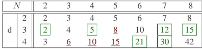
Figure
Documents relatifs
The direct cost includes software, hardware, its maintenance, staffing and training; the benefits include savings realized due to the reduction in delivery charges, travels,
At the heart of a good understanding of any quantum control problem, in- cluding the efficiency, accuracy, and stability of quantum control experiments as well as simulations,
The signifi cant item-to-scale correlations between the English and French online versions of the SOS-10 suggest items were tapping into the construct of psychological well-being
159 “Vamos segurar nossas pontas!” Paisagens em movimento e domínio sobre os lugares no rio Arapiuns Mostrei que as mudanças na paisagem ligadas às interações entre vários
n’importe quoi peut, suivant les cas, agir à cet égard comme une "cause occasionnelle" ; il va de soit que celle-ci n’est pas une cause au sens propre de ce mot, et
All these arguments suggest that individual incentives to challenge a patent may be rather low. The probabilistic nature of patent protection and the low individual incentives
ﻰﻠﻋ ﺎﻨودﻋﺎﺴ و ﺎﻨﻨﻴوﻜﺘ لﻴﺒﺴ ﻲﻓ دوﻬﺠﻝا لﻜ اوﻝذﺒ نﻴذﻝا ةذﺘﺎﺴﻷا ﻊﻴﻤﺠ رﻜﺸا ﺎﻤﻜ ﺔﻓرﻌﻤﻝا و مﻠﻌﻝا بﺎﺴﺘﻜا. صﺼﺨﺘ قوﻘﺤ رﺘﺴﺎﻤﻝا ﺔﺒﻠط ﻲﺌﻼﻤز لﻜ ﻰﻝإ صﻝﺎﺨﻝا
