HAL Id: halshs-00622325
https://halshs.archives-ouvertes.fr/halshs-00622325
Preprint submitted on 12 Sep 2011
HAL is a multi-disciplinary open access
archive for the deposit and dissemination of
sci-entific research documents, whether they are
pub-lished or not. The documents may come from
teaching and research institutions in France or
L’archive ouverte pluridisciplinaire HAL, est
destinée au dépôt et à la diffusion de documents
scientifiques de niveau recherche, publiés ou non,
émanant des établissements d’enseignement et de
recherche français ou étrangers, des laboratoires
Measuring Poverty Without The Mortality Paradox
Mathieu Lefebvre, Pierre Pestieau, Grégory Ponthière
To cite this version:
Mathieu Lefebvre, Pierre Pestieau, Grégory Ponthière. Measuring Poverty Without The Mortality
Paradox. 2011. �halshs-00622325�
WORKING PAPER N° 2011 – 30
Measuring Poverty Without The Mortality Paradox
Mathieu Lefebvre
Pierre Pestieau
Grégory Ponthière
JEL Codes: I32
Keywords: premature mortality, income-differentiated mortality, poverty
measurement, censored income profile
P
ARIS
-
JOURDAN
S
CIENCES
E
CONOMIQUES
48, BD JOURDAN – E.N.S. – 75014 PARIS TÉL. : 33(0) 1 43 13 63 00 – FAX : 33 (0) 1 43 13 63 10
Measuring Poverty Without The Mortality
Paradox
Mathieu Lefebvre, Pierre Pestieau
yand Gregory Ponthiere
zAugust 17, 2011
Abstract
Under income-di¤erentiated mortality, poverty measures re‡ect not only the "true" poverty, but, also, the interferences or noise caused by the survival process at work. Such interferences lead to the Mortality Paradox: the worse the survival conditions of the poor are, the lower the measured poverty is. We examine several solutions to avoid that paradox. We identify conditions under which the extension, by means of a …ctitious income, of lifetime income pro…les of the prematurely dead neutralizes the noise due to di¤erential mortality. Then, to account not only for the "missing" poor, but, also, for the "hidden" poverty (premature death), we use, as a …ctitious income, the welfare-neutral income, making indi¤erent between life continuation and death. The robustness of poverty measures to the extension technique is illustrated with regional Belgian data.
Keywords: premature mortality, income-di¤erentiated mortality, poverty measurement, censored income pro…le.
JEL classi…cation code: I32.
University of Liege.
yUniversity of Liege, CORE, PSE and CEPR.
zEcole Normale Superieure, Paris, and Paris School of Economics. [corresponding author]
Contact: ENS, 48 Bd Jourdan, Building B, 2nd ‡oor, O¢ ce B, 75014 Paris, France. Tel: 0033-1-43136204. E-mail: [email protected]
1
Introduction
In An Essay on the Principle of Population (1798), Malthus emphasized that the population is a social product, whose size adjusts to the prevalence of poverty through two kinds of population "checks". On the birth side, poverty reduces fertility through parental anticipations about future di¢ culties to raise children (i.e. "preventive checks"). Moreover, poverty leads to premature deaths within the low income classes (i.e. "positive checks").
Given the underdeveloped state of social statistics at Malthus’s time, the existence of population checks was more a conjecture than a scienti…c result. However, in the recent years, empirical studies con…rmed the existence of posi-tive population checks, under the form of a relationship between income and life expectancy.1 On average, individuals with higher incomes have, ceteris paribus,
a longer life than individuals with lower incomes.2
Income-di¤erentiated mortality raises a twofold challenge for the measure-ment of poverty. Actually, the two aspects of poverty measuremeasure-ment underlined by Sen (1976) are a¤ected: on the one hand, the identi…cation of the poor within the population; on the other hand, the construction of an index aggregating and weighting the information available on the identi…ed poor.
Regarding the identi…cation of the poor, income-di¤erentiated mortality leads to a paradox. Poor persons tend to die, on average, earlier than non-poor persons. Hence, usual poverty measures, which focus on living individuals, do not count the "missing" poor, and, thus, re‡ect not only the "true" poverty, but, also, the interferences or noise due to income-di¤erentiated mortality.3
Those interferences push towards a lower poverty estimate. As a consequence, poverty measures tend to underestimate the "true" poverty.4 That problem can
be called the Mortality Paradox: the worse the survival conditions faced by the poor are, the lower the measured poverty is. That result is paradoxical, since poverty measures should be increasing - or, at least, non-decreasing - in the premature mortality faced by the poor due to their low income.
Income-di¤erentiated mortality raises also an important challenge regarding the treatment of the informational basis relevant for the measurement of poverty. Undoubtedly, a shorter life is a major source of deprivation. Hence, if individuals with lower incomes face also a higher mortality, it is hard to ignore this when measuring poverty. But if one takes premature death as a part of the poverty phenomenon to be measured, then a major issue concerns the weighting of the two dimensions under study: income and longevity.
This paper focuses on the challenges raised by income-di¤erentiated mor-tality for the measurement of poverty, by re-examining the Mormor-tality Paradox
1The same cannot be said on the birth side, where the observed fertility transition has
in…rmed the existence of preventive population checks. Indeed, to explain the fertility decline, the substitution e¤ect related to the rise in productivity must have overcome the income e¤ect.
2See, among others, Duleep (1986), Deaton and Paxson (1998), Deaton (2003), Jusiot
(2003) and Salm (2007). One exception is Snyder and Evans (2006), who show that high income groups face, ceteris paribus, a higher mortality than low-income groups.
3The existence of "missing poor" due to income-di¤erentiated mortality is quite similar to
the existence of "missing women" because of gender discriminations (see Sen 1998).
4This problem is general, and concerns all poverty measures, including the recent
multi-dimensional poverty indexes. For instance, the Human Poverty Index (UNDP 1997), which includes, as dimensions, the probability of not surviving to ages 40 or 60, faces the paradox, since poor persons who survive until 40 or 60 years and then die will not be counted as poor after their death, so that a poverty-related death reduces the poverty measure.
and its solutions. For that purpose, we …rst develop a 2-period model with income mobility and income-di¤erentiated mortality, and study the conditions under which the Mortality Paradox occurs. We propose also a solution to it: the extension, by means of a …ctitious income, of lifetime income pro…les of the prematurely dead. Then, in a second stage, we argue that a natural candidate for the …ctitious income is the welfare-neutral income, i.e. the income making an agent indi¤erent between further life with that income and death. Finally, we use Belgian data to estimate the bias induced by the Mortality Paradox, and to evaluate the robustness of adjusted poverty measures to the extension of income pro…les. This allows us to decompose the adjustment into counting the "missing" persons and valuing premature death as a part of poverty.
At this stage, it is important to relate our paper to the existing literature on poverty measurement. As far as we know, there exists only one paper, by Kanbur and Mukherjee (2007), which proposed a solution to the Mortality Paradox. They recommend, when computing poverty measures, to count the prematurely dead poor persons as if they were still alive, and to truncate their lifetime income pro…les by means of a …ctitious income depending on past incomes. Our paper complements that contribution on three grounds. Firstly, whereas Kanbur and Mukherjee propose general rules for the selection of a …ctitious income, we argue, on the contrary, that the …ctitious income should be equal to a particular level: the welfare-neutral income. Secondly, while Kanbur and Mukherjee only truncate the income pro…les among the poor population, we propose to do it for all "missing" persons. Thirdly, whereas Kanbur and Mukherjee’s paper is purely theoretical, we provide empirical estimates of the size of the bias induced by the Mortality Paradox, as well as an empirical study of the robustness of adjusted old-age poverty measures to the extension technique used.
Anticipating our results, we …rst show how, under income-di¤erentiated mor-tality, standard old-age poverty rates are subject to the Mortality Paradox. We show that, when a …ctitious income lower than the poverty line is assigned to prematurely dead poor individuals only, the adjusted poverty rate is robust to variations in survival conditions, and, thus, avoids the Mortality Paradox. Then, we consider the construction of alternative adjusted poverty measures, which count a premature death as an aspect of deprivation and poverty. Such measures, instead of being invariant to a worsening of survival conditions, are increasing with the strength of positive population checks. That alternative solution to the Mortality Paradox consists of assigning, to all prematurely dead persons, a …ctitious income equal to the welfare-neutral income. Finally, we show, on the basis of Belgian regional data, that, while the addition of the "missing" persons with …ctitious incomes equal to the incomes when being alive only raises the poverty rates by about one point, the assignment of a …ctitious income equal to the welfare-neutral income raises poverty rates by 6-7 points. This suggests that taking the "hidden" burden of premature death into account is a much bigger correction than merely counting the "missing" poor.
The paper is organized as follows. Section 2 studies the measurement of poverty in a model with income mobility and income-di¤erentiated mortality, and identi…es conditions under which truncating income pro…les of the prema-turely dead prevents the Mortality Paradox. Section 3 explores a particular extension, which relies on the welfare-neutral income. Section 4 illustrates, on the basis of regional Belgian data, the Mortality Paradox and the robustness of poverty measures to the extension method. Conclusions are drawn in Section 5.
2
Poverty measure and income-based mortality
2.1
The framework
Let us consider a two-period model, where a cohort, of size N 2 N, lives the young age (…rst period) for sure, whereas only some fraction of the population will enjoy the old age (second period).5
There exists a …nite number K 2 N of possible income levels (K > 1). The set of possible income levels is: Y = fy1; :::; yKg. For the ease of presentation,
we assume that income levels are indexed in an increasing order, so that:
y1< ::: < yK (1)
The number of young individuals with income yi 2 Y is denoted by n1i.6 We
denote by n1the vector of size K, whose entries are n1k for k = 1; :::; K. The probability of survival to the old age, denoted by , depends on the income when being young. Following the literature, we assume that a higher in-come when being young leads to higher survival chances.7 Hence income-speci…c
survival probabilities, which take K distinct values, are ranked as follows:
1< ::: < K (2)
We denote by the vector of size K whose entries are the income-speci…c sur-vival probabilities k, for k = 1; :::; K. The number of surviving old individuals
with income yi 2 Y is denoted by n2i.8 We denote by n2the vector of size K,
whose entries are n2
k for k = 1; :::; K.
Denoting by ij the probability that a young agent with income yi enjoys,
in case of survival, an income yj at the old age, the income mobility can be
described, conditionally on survival, by the right stochastic matrix :
= 0 B B @ 11 12 ::: 1K 21 22 ::: 2K ::: ::: ::: ::: K1 K2 ::: KK 1 C C A (3)
The income mobility matrix concerns individuals who live the two periods. As such, this does not take premature death into account, and, thus, leads to an incomplete representation of the dynamics of income distribution.
Actually, the dynamics of income distribution can be represented by means of the transition matrix M, of size K K, which describes how the income distribution at the young age determines the income distribution at the old age:
n2= M0n1 (4)
The transition matrix M is:
M= 0 B B @ 1 11 1 12 ::: 1 1K 2 21 2 22 ::: 2 2K ::: ::: ::: ::: K K1 K K2 ::: K KK 1 C C A (5)
5Our argument is robust to the number of life-periods. We focus here on a two-period
framework to simplify the presentation without unnecessary material.
6By construction, we have: PK
k=1n1k= N.
7See Duleep (1986), Deaton and Paxson (1998), Jusiot (2003) and Salm (2007). 8By construction, we have: PK
k=1n2k=
PK k=1 kn1k.
The M matrix fully describes the trajectories of individuals in our econ-omy. The lifecycle trajectory depends on survival probabilities and on income transition probabilities, which are correlated in terms of rank. We can easily de-compose the matrix M into its two components: the income mobility component and the survival process component:
M= (6)
where 10
K, 1K being the identity vector of size K, while the symbol
refers to the Hadamard product, that is, the entrywise product of two matrices. The M matrix includes, as a special case, the situation where there is no premature death (i.e. i = 1 for all i). In that case, the matrix M vanishes
to the income mobility matrix . Alternatively, if there is no mobility over the lifecycle (i.e. ii= 1 for all i), the matrix M is a diagonal matrix with survival
probabilities i as entries.
2.2
The Mortality Paradox
The Mortality Paradox is a general problem faced by various types of poverty measures. It refers to an undesirable sensitivity of poverty measures to income-di¤erentiated mortality. That paradox can be stated as follows: the worse the survival conditions faced by the poor are, the lower the measured poverty is.
The origin of that paradox has to do with the selection mechanism that is at work under income-di¤erentiated mortality. Survival laws act as a selection process: poor individuals die, on average, earlier than non-poor persons. This implies that poor persons become, with the mere passage of time, relatively less numerous than non-poor persons, yielding a lower measured poverty. That result is paradoxical, since the measured poverty should not decrease because of the mere existence of positive population checks. Actually, income-di¤erentiated mortality can be regarded as creating some interferences or a noise preventing the measurement of the "true" poverty.
To illustrate the Mortality Paradox, let us focus on the simplest measures of poverty, i.e. head-count ratios, which measure poverty by counting the number of individuals whose incomes are below a (…xed) poverty threshold yP 2 Y .
De…nition 1 Assume an economy with income distribution ni at age i = 1; 2. If yP 2 Y is the poverty threshold, the poverty rate at age i is:
Pi= PP 1
j=1 nij
PK k=1nik
The old-age poverty rate P2is subject to the Mortality Paradox. To see this,
let us consider the following example. In a …rst situation n1; ; , individuals
who are poor at the young age survive to the old age with positive probabilities 0 < k < 1 for k < P , and there is no income mobility (i.e. jj = 1 for all
j). In the second situation n10; 0; , individuals who are poor at the young age do not survive to the old age: 0
k = 0 for k < P , and there is no income
mobility (i.e. jj= 1 for all j). Writing the old-age poverty rate as:
P2= PP 1 j=1 n2j PK k=1n2k = PK j=1 jn1j PP 1 l=1 jl PK k=1 kn1k (7)
we obtain the following two measures of poverty, denoted by P2 for the …rst
situation and by P20 for the second one:
PP 1 j=1 jn1j PK k=1 kn1k > PP 1 j=1 0jn1j0 PK k=1 0kn1k0 = 0
The old-age poverty rate is larger in the …rst situation than in the second one. The reason has nothing to do with the level of poverty at the young age, which could take any possible value; nor does it have anything to do with mobility (which is absent in the two situations); nor does it have anything to do with a change in the poverty threshold yP, which is supposed to be the same in the
two situations under study.9 Actually, the lower level of measured poverty at
the old age in the second situation is the mere outcome of income-di¤erentiated mortality. The strong positive population checks at work in the second situation have made old-age poverty vanish to - apparently - nothing.
The fact that a more severe income-based mortality reduces the measured poverty is paradoxical. Poverty indexes should show us the extent of poverty, and not be disturbed by the noise due to income-based mortality. Hence the Mortality Paradox invites a re…nement of poverty measures.
To avoid that paradox, one solution consists of imposing that poverty mea-sures exhibit some independence with respect to survival conditions. The follow-ing property, entitled Robustness to Mortality Changes, captures that intuition. Condition 1 (Robustness to Mortality Changes) A poverty measure Pi
satis…es Robustness to Mortality Changes if and only if a deterioration of the survival conditions of the poor leaves the measured poverty unchanged:
If k>
0
k for some k < P k = 0k for other k K
, then Pi = Pi0:
Robustness to Mortality Changes requires poverty measures to be invariant to a deterioration of the survival conditions faced by the poor. Whereas that property requires to observe the impact of a change in survival conditions on the poverty measure, a simpler way to avoid the Mortality Paradox consists of imposing that a poverty measure depends only on two things: (1) the level of poverty at younger ages; (2) the matrix of income mobility over the lifecycle. That simpler requirement is captured by the following property.
Condition 2 (No Mobility Same Poverty) A poverty measure Pi satis…es No Mobility Same Poverty if and only if, in the absence of income mobility, the measured poverty is constant across the lifecycle:
If ii= 1 for all i, then P1= P2:
The No Mobility Same Poverty condition states that, if we consider an econ-omy without mobility, the poverty rate should be constant across the lifecycle. That condition rules out the Mortality Paradox. Actually, this is also equivalent to the Robustness to Mortality Changes condition.
Lemma 1 Robustness to Mortality Changes and No Mobility Same Poverty are equivalent conditions.
Proof. See the Appendix.
That equivalence result is useful, since this will allow us, when studying whether a poverty measure satis…es Robustness to Mortality Changes or not, to focus on the hypothetical case where there is no income mobility, and to check whether the poverty rate is constant or not along the lifecycle.
Let us now examine whether poverty rates satisfy those conditions or not. As it is shown below, the old-age poverty rate P2 does not satisfy the Robustness to Mortality Changes condition. The old-age poverty rate is actually subject to the interferences induced by income-di¤erentiated mortality.
Proposition 1 P2 does not satisfy Robustness to Mortality Changes.
More-over, we have, in the absence of income mobility, that: P1> P2.
Proof. See the Appendix.
The old-age poverty rate is not robust to a deterioration of the survival conditions faced by the poor. The old-age poverty rate P2 is thus subject to
the Mortality Paradox. Moreover, by the above lemma, we know that P2 does
not satisfy No Mobility Same Poverty: P2is inferior to the P1under no income
mobility. The reason is that poor individuals tend to die earlier than non-poor persons, pushing the old-age poverty rate below the young age poverty rate.
2.3
A general solution to the Mortality Paradox
The reason why poverty measures su¤er from the Mortality Paradox has to do with the fact that, once dead, poor persons disappear from the population. Therefore, as suggested by Kanbur and Mukherjee (2007), a solution to the Mortality Paradox comes from the extension of lifetime income pro…les, to take into account the persons subject to premature mortality.
The underlying idea is the following. Instead of computing old-age poverty measures on the basis of the surviving persons only, one should do as if all individuals are still alive at the old age, and bene…t from some income. For that purpose, lifetime income pro…les must be extended, to assign some income to prematurely dead persons.
The assignment of a …ctitious income to the premature dead implies that we have now two, instead of one, income transition matrices: one for individuals who survived to the old age, i.e. , and one for those who did not survive. We will denote that latter income transition matrix by , of size K K:
= 0 B B @ 11 ::: ::: 1K ::: ::: ::: ::: ::: ::: ::: ::: K1 ::: ::: KK 1 C C A (8)
where ijis the probability, for an individual with income yiwhen being young,
to have a …ctitious income ei = yj assigned to him when he is dead.
The adjusted old-age poverty rate, denoted by ^P2, can be written as:
^ P2= PK i=1 in1i PP 1 j=1 ij +PKi=1(1 i)n1i PP 1 j=1 ij PK k=1n1k (9)
The …rst term of the numerator is standard: it counts the poor individuals among the old (surviving) population. But the second term is less standard: it counts the poor individuals among those who did not survive, their …ctitious incomes being assigned to them through the matrix .
The adjusted poverty rate ^P2 can take distinct forms, depending on: (1)
whether the assignment of …ctitious incomes concerns all individuals or only the initially poor; (2) whether …ctitious incomes exceed or are below the poverty line yP. Those two features of the extension are captured by the matrix .
The next proposition examines the conditions on under which ^P2avoids the Mortality Paradox. As above, we rely here on the No Mobility Same Poverty (i.e. NMSP), since we know, by our lemma, that a violation of that property leads to a violation of Robustness to Mortality Changes.10
Proposition 2 I: A …ctitious income ei is assigned to the dead poor only.
- Ia: If ei< yP for all i, ^P2 satis…es NMSP: ^P2= P1.
- Ib: If ei< yP for i < R P and ei yP for i R, ^P2 does not satisfy
NMSP: ^P2< P1.
- Ic: If ei yP for all i, ^P2 does not satisfy NMSP: ^P2< P1.
II: A …ctitious income ei is assigned to all dead individuals.
- IIa: If ei< yP for all i, ^P2 does not satisfy NMSP: ^P2> P1.
- IIb: If ei< yP for i < R P and ei yP for i R, ^P2 does not satisfy
NMSP: ^P2? P1.
- IIc: If ei yP for all i, ^P2 does not satisfy NMSP: ^P2< P1.
Proof. See the Appendix.
When …ctitious incomes are assigned only to the prematurely dead poor persons, and when all …ctitious incomes are lower than the poverty line, ^P2
satis…es the No Mobility Same Poverty, and, by our lemma, exhibits Robustness to Mortality Changes, and, thus, avoids the Mortality Paradox.
That case - case Ia - is quite speci…c, and - even slight - departures from this will generally imply a lack of robustness of the old-age poverty rate to changes in survival conditions. Two kinds of sensitivity can arise, and these do not have the same relationship with the Mortality Paradox.
On the one hand, if the …ctitious income exceeds the poverty threshold (i.e. cases Ib, Ic, IIc), the old-age poverty rate does not satisfy Robustness to Mor-tality Changes, and is subject to the MorMor-tality Paradox. In that case, ^P2 is,
despite the adjustment, lower than P1, since only a subgroup of the prematurely dead poor persons are counted as poor in the adjusted measure.
On the other hand, if …ctitious incomes are assigned to all prematurely dead persons (i.e. cases IIa), ^P2 is not invariant to mortality changes. ^P2 is then
higher than the poverty rate at the young age, because we count all prematurely dead persons as poor. Hence the Mortality Paradox does not hold here. It is quite the opposite, since ^P2does not only count the "missing" poor, but counts
also premature death as a part of the poverty phenomenon to be measured.11
1 0We assume, for the simplicity of presentation, that the poverty line y
P is invariant to the
adjustment. Alternatively, if one considers a relativistic view of poverty, it could be argued that the adjustment a¤ects also the poverty line. Given that this second-order e¤ect depends on the precise way in which the poverty line is computed, we leave that discussion to the empirical example of Section 4.
Finally, let us notice a special case where the two reasons why ^P2violates No
Mobility Same Poverty go in opposite directions. It can be shown that, under particular circumstances, those reasons cancel each other, making ^P2satisfy No
Mobility Same Poverty.
Corollary 1 When (1) a …ctitious income is assigned to all prematurely dead persons; (2) the …ctitious income is inferior to yP for all short-lived poor
individ-uals, and is superior to yP for all short-lived non-poor individuals, ^P2 satis…es
No Mobility Same Poverty. That case coincides with case IIb with R = P . Proof. See the Appendix.
In that case, we know also, by the equivalence lemma, that ^P2is robust to a deterioration of the survival conditions faced by the poor, so that ^P2 avoids the Mortality Paradox.12
In sum, this section shows that it is possible to escape from the Mortality Paradox by truncating the lifetime income pro…les of the prematurely dead. That extension can be done in various ways, but, if one wants poverty measures to be invariant to changes in mortality, the extension should concern either only the prematurely dead poor individuals, with …ctitious incomes below the poverty threshold, or every prematurely dead, but with …ctitious incomes below the poverty line only for prematurely dead poor individuals.
3
The extension of income pro…les revisited
The previous section identi…ed conditions under which truncating income pro-…les of the dead makes poverty measures avoid the Mortality Paradox. That solution, although appealing, faces some criticisms, which concern both the se-lection and meaningfulness of the …ctitious incomes used in the extension.
A …rst criticism is that, even if one sticks to the extension described above, there exist not a single, but numerous ways to truncate the lifetime income pro…les of the prematurely dead. The problem is that the resulting poverty es-timates are likely to be strongly sensitive to the chosen …ctitious income ei. The
closer ei is to yP, the lower the measured poverty is. Hence, the measurement
of poverty in real environments requires more precise information.13
A second criticism concerns the extent to which premature mortality per se matters for poverty measurement. Once lifetime income pro…les are extended, the …ctitious income enters the poverty measure as if it was an income enjoyed by a living person. This amounts to regard as equivalent two situations that
1 2That special case includes the situation where the matrix assigning …ctitious incomes, i.e.
, coincides with the income mobility matrix . Indeed, in that case, we have: ^ P2= PK i=1n1i PP 1 j=1 ij PK k=1n1k
It is easy to check that this adjusted poverty rate satis…es No Mobility Same Poverty.
1 3That critique applies not only to the extension discussed above, but, also, to what was
proposed by Kanbur and Mukherjee (2007). According to them, the …ctitious income has to satisfy three properties: (1) it is increasing in the past income (i.e. yi> yi 1 =) ei> ei 1);
(2) it cannot exceed the past income (i.e. ei yi); (3) agents who are not poor when being
alive should not be counted as poor after the extension (i.e. ei yP when yi> yP). Those
conditions imply that the poverty measure falls under case Ia, and escapes from the Mortality Paradox. However, those conditions are too general for measurement exercises.
are quite di¤erent: on the one hand, being alive with some income yi, and, on
the other hand, being dead with a …ctitious income ei equal to yi. Hence the
extension of lifetime income pro…les has a double e¤ect. This does not only allow to count some - otherwise missing - poor in the measure of poverty. The extension assigns also some weights to two dimensions of poverty (income and longevity). Such a weighting exercise cannot remain implicit, but should have some explicit (welfare) foundations.
Those two criticisms invite a method to select a particular …ctitious income, and to solve the trade-o¤s, in terms of poverty measurement, between low in-comes and short lives. This is the task of the present section.
3.1
A welfare-neutral …ctitious income
To overcome those two criticisms, we propose here to carry out the computation of …ctitious incomes on the basis of individual preferences on lifetime income pro…les. More precisely, we propose to solve those problems by selecting a particular …ctitious income: the welfare-neutral income. This is de…ned as the hypothetical income that would make an individual indi¤erent between, on the one hand, further life with that income, and, on the other hand, death.
The reliance on individual preferences requires some justi…cations. Actually, the Mortality Paradox is a paradox only to the extent that premature death is a part of the poverty phenomenon to be measured. If premature death had nothing to do with poverty, then there would be nothing paradoxical in having poverty measures decreasing once survival conditions deteriorate. But the will to overcome the Mortality Paradox pushes us de facto in the …eld of multidimen-sional poverty measurement. Hence, it is hard to ignore individual preferences as providing an adequate informational basis for weighting the two dimensions of poverty (income and longevity). Indeed, if the level of the …ctitious income contributes to assign a speci…c "weight" re‡ecting the contribution of premature death to poverty, then using individual preferences is the natural way to solve that weighting exercise.
To de…ne that welfare-neutral income, let us assume that individuals have well-de…ned preferences over all possible lifetime income pro…les, and that those preferences can be represented by a non-decreasing function U ( ):14
U (u1i; u2j) (10)
where ut
i is the value assigned by a state-dependent temporal utility function at
period t under temporal income yi:
uti = u(yi) if the individual is alive at that period
if the individual is not alive at that period (11) where u( ) is increasing, while is the utility of being dead.15
On the basis of that, one can de…ne the "welfare-neutral" income as follows. De…nition 2 For an individual with income yi2 Y with premature death, the
welfare-neutral income yi is the hypothetical income that makes him indi¤ erent
between life continuation and death:
U (u(yi); ) = U (u(yi); u(yi))
1 4For the sake of simplicity, we assume that preferences are uniform. 1 5That number is, in most applications, set to zero (see below).
Note that whether the welfare-neutral income yi is higher or lower than the
income when alive yi is an open issue. The answer depends on the individual’s
preferences (i.e. the shape of the functions U ( ) and u ( )), and on how poor he was when alive (i.e. yi enjoyed at the young age).
Having de…ned the welfare-neutral income yi, let us now explain why it is
a plausible candidate for the extension of lifetime income pro…les of the pre-maturely dead. For that purpose, we will show how the welfare-neutral income provides a solution to the two criticisms formulated above, by considering the welfare consequences of the extension of lifetime income pro…les.
Actually, when one truncates an agent’s income pro…le (yi; 0) with a …ctitious
income ei, this amounts to do as if that person was still alive during that period,
and enjoyed an income ei. Thus, the hypothetical situation after extension can
be better or worse than the actual situation depending on whether:
U (u(yi); )7 U(u(yi); u(ei)) (12)
If the RHS exceeds the LHS, the person would have preferred living one more period with the …ctitious income rather than dying after the young age. If the LHS exceeds the RHS, the person thinks that his actual life is better than the same life with the addition of one period with income ei. In the former case, the
extension of the income pro…le amounts to do as if the person had enjoyed a better life than the one he actually enjoyed. In the latter case, it is the opposite. But in any case, the extension disconnects the measurement of poverty from the measurement of welfare, which is problematic.
To illustrate this, let us compare three cases.
Case A: an individual with income yi < yP dies after period 1, and no
extension is made in the poverty measure.
Case B: an individual with income yi < yP dies after period 1, but his
income pro…le is extended by means of the income ~ei< yP such that:
U (u(yi); ) < U (u(yi); u(~ei))
Case C: an individual with income yi < yP dies at the end of period 2,
and enjoys the income yj= ~ei< yP at the old age.
The measured poverty is lower in Case A than in Case B. The measured poverty is also lower in Case A than in Case C, since Case C is equivalent to Case B for the measurement of poverty. Hence we have: P2A < P2B = P2C. In welfare terms, Cases A and B are equivalent, since these di¤er only in how poverty is measured, and are exactly the same otherwise. Case C dominates the other cases in welfare terms (because of the above inequality). Thus we have: UA = UB < UC. Hence, the death of the individual, i.e. the passage
from C to B, reduces his welfare, but does not change the measured poverty. This is quite problematic. Clearly, if a society undergoes an epidemy, so that many individuals shift from Case C to Case B, it is hard to claim, despite the fall in social welfare, that poverty is, at the end, the same as if the epidemic had not occurred. Such a claim is surely subject to the Mortality Paradox. The constancy of the measured poverty despite a change in living conditions is acceptable only if that change is welfare-neutral.
Actually, there exists only one level of the …ctitious income ei that avoids
that problem. It is the "welfare-neutral" income yi. It is easy to see that, when
ei = yi, there is no discrepancy between poverty measurement and welfare
measurement. Indeed, if we now assume ei = yi, we still get that poverty is
larger under Cases B and C than under Case A, i.e. PA< PB= PC. In welfare
terms, we have that Cases A and B are still equivalent (since the only change concerns how poverty is measured), but that welfare in Case C is also equal to what it is in Case B, since, by de…nition, survival with the …ctitious income does not constitute a welfare improvement. Hence we have: UA= UB = UC.
Thus, poverty is the same in B and C, and welfare too. Here there is nothing shocking in having a constant poverty measure despite the occurrence of an event such as an epidemic, since that event is here welfare-neutral, unlike what prevailed above. Here the comparison of Cases B and C consists of comparing the emergence of an epidemic with its avoidance at the cost of extreme misery (leading individuals to indi¤erence between life and death). Those two situations are equivalent in terms of poverty, and the Mortality Paradox does not arise.
In sum, the use of the welfare-neutral income as a …ctitious income allows us to base the extension on a speci…c …ctitious income, as well as to avoid a discrepancy between the measurement of poverty and the measurement of welfare. As such, this brings an appealing solution to the Mortality Paradox.
3.2
A speci…c case: time-additive welfare
The "welfare-neutral" …ctitious income yi depends on the postulated
prefer-ences, which can take various forms. However, under standard time-additive lifetime welfare, the welfare-neutral income yi has two convenient properties.
On the one hand, it is unique; on the other hand, it is independent from past income.
To see this, let us assume that lifetime welfare takes a time-additive form: U (u1i; u2j) = u1i + u2j (13) where is a time preference factor (0 < < 1). Then, if the utility of death is normalized to zero (i.e. = 0), we have
U (u1i; 0) = u1i + 0 = u(yi) (14)
Hence, the welfare-neutral income yi, is implicitly de…ned by:
u(yi) = 0 (15)
An additional life-period with income larger than yiis worth being lived, whereas
a life-period with income lower than yi is not. Under that speci…cation, the
…ctitious income yi is such that temporal welfare is zero, that is, equivalent
to the temporal welfare associated to death. Thus, in that case, the welfare-neutral income yi is the same for all past income levels. In the rest of this
section, we will denote it by yN. As a consequence, it appears that, under
standard time-additive lifetime utility, the welfare-neutral income level is unique and independent from past incomes. Note that those properties way not hold under alternative, less standard, preferences.16
3.3
Properties of the new adjusted poverty measure
Let us now study whether adjusted poverty measures based on welfare-neutral …ctitious incomes are robust to changes in survival conditions. Remind that the adjusted old-age poverty rate ^P2is now computed by assigning a single value -i.e. the welfare-neutral …ctitious income - for the second-period income for all prematurely dead individuals.
As explained above, whether the welfare-neutral …ctitious income lies above or below the past income when alive depends on individual preferences, and on the past income level. Therefore the transition matrix can take various forms. Note, however, that, in the case of time-additive lifetime welfare, the welfare-neutral income takes a single value, denoted by yN, which is independent from
past incomes. Hence takes a simple form, where ij = 0 for j 6= N and iN = 1 for all i, and the adjusted poverty rate ^P2can be written as:
^ P2= PK i=1 in1i PP 1 j=1 ij +PKi=1(1 i)n1i PK k=1n1k if yN < yP ^ P2= PK i=1 in1i PP 1 j=1 ij PK k=1n1k if yN yP
In the former case, the prematurely dead persons are all counted as poor. In the latter case, they all disappear from the poverty measure. The interpretation of those two cases is as follows. When yN < yP, an individual enjoying an income
equal to the poverty line still prefers that life to death, whereas, when yN yP,
the poverty threshold is lower than the welfare-neutral income level, revealing that the misery makes life not worth being lived.
To identify the conditions under which the so-constructed adjusted poverty measure ^P2 is subject to the Mortality Paradox, we will, as above, examine
whether ^P2 satis…es No Mobility Same Poverty (NMSP), since it is a simple
way to see whether ^P2 is robust to changes in survival conditions.17
Proposition 3 Consider an economy with time-additive lifetime welfare. Under yN < yP, ^P2 does not satisfy NMSP: ^P2> P1.
Under yN yP, ^P2 does not satisfy NMSP: ^P2< P1.
Proof. See the Appendix.
Thus, once the …ctitious income takes its welfare-neutral level and is as-signed to all prematurely dead individuals, the adjusted poverty rate does not lived (see Broome 2004, p. 228):
U (u1i; u2j) = min u1i; u2j
U (u1i; u2j) = max u1i; u2j
Under the min speci…cation, yi is such that u(yi) u1i, which implies yi yi, but does not
allow us to say more. On the contrary, under the max speci…cation, we have yi yi. Thus
the uniqueness and the independence of the welfare-neutral income from past income are not general properties, but only nice corollaries of standard time-additive lifetime welfare.
1 7As above, we assume here that the poverty line y
P is invariant to the adjustment made
satisfy No Mobility Same Poverty, and, by the equivalence lemma, also violates Robustness to Mortality Changes. That lack of robustness occurs, since the extension based on the welfare-neutral …ctitious income amounts to count early deaths as a source of the poverty phenomenon to be measured. The sensitivity of adjusted poverty measure to survival conditions has two meanings.
When yN lies below the poverty threshold yP, all premature deaths are
regarded as a source of poverty, and this explains why ^P2 is sensitive to a de-terioration of survival conditions. Thus, adjusted poverty measures, instead of being invariant to changes in income-based mortality, take di¤erential mortal-ity into account, in the opposite way as standard poverty measures do. This explains why ^P2 violates the Robustness to Mortality Changes in that case.
If, on the contrary, the welfare-neutral income level exceeds the poverty threshold, the adjusted poverty measure at the old age is lower than the poverty measure at the young age. The intuition is that, in that case, life is not worth being lived for all poor persons. As a consequence, in that context, prema-ture death cannot be counted as something causing poverty, and the Mortality Paradox is hardly relevant under those circumstances.
In sum, this Section proposed to overcome the Mortality Paradox by trun-cating lifetime income pro…les of the prematurely dead by means of the welfare-neutral income. The use of the welfare-welfare-neutral income as a …ctitious income can be defended on two grounds. First, the computation of an income that yields indi¤erence between life and death leads, under standard preferences, to a unique value for the …ctitious income. Such a uniqueness is most welcome when we consider the empirical measurement of poverty, which is strongly sen-sitive to the …ctitious income (see below). Second, the so-computed …ctitious income can also, thanks to its welfarist foundations, sort out trade-o¤s between income and longevity. As such, this adjustment of poverty measures does more than counting the "missing" individuals; it also takes into account a "hidden" -but central - part of the poverty phenomenon to be measured: premature death.
4
Old-age poverty in Belgian regions
Let us now illustrate the downward bias due to the Mortality Paradox, and the sensitivity of adjusted old-age poverty measures to the extension of income pro…les. For those purposes, we will use data from Belgium and its regions.
4.1
The data
We use raw poverty measures coming from the European household survey EU-SILC for the year 2006 (EU, 2006). Regarding longevity data, the empirical study of the Mortality Paradox ideally requires lifetables di¤erentiated according to income groups. Such lifetables are not available, but these are derived from education-speci…c lifetables from Deboosere et al. (2009).18
Since the Mortality Paradox is about the e¤ect of di¤erentiated survival conditions on poverty measurement, one can expect that measurement biases induced by income-di¤erentiated mortality are more negligible at younger ages. Therefore, to estimate the biases due to di¤erentiated mortality, we will focus
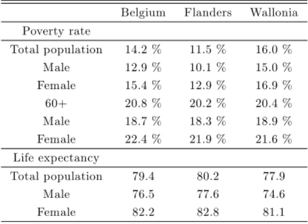
on the measurement of poverty in the population aged 60 or more. Table 1 presents the head-count poverty rates by region and by age groups in 2006.
Poverty is higher among those of age 60 and more than among the total population. While the total poverty rate is 14.2 %, the proportion of poor elderly is 20.8 %. There exist also large di¤erences between men and women. Whatever the region and the age group are, poverty rates are larger among women than among men. That gender poverty gap is particularly high above the age of 60. Table 1 highlights also a big di¤erence between Flanders and Wallonia. That gap is important among the younger generations, but tends to vanish at older age, thanks to the (nationwide) pension system.
Table 1 also shows life expectancy di¤erentials between men and women, and between Flanders and Wallonia. Whereas the gender gap in life expectancy is well documented, the geographical gap is more surprising. Indeed, although both regions are geographically close to each other, life expectancy at birth in Wallonia is shorter than in Flanders, by about 2 years and a half.
Table 1 : Poverty and life expectancy in Belgium1 9
Belgium Flanders Wallonia Poverty rate Total population 14.2 % 11.5 % 16.0 % Male 12.9 % 10.1 % 15.0 % Female 15.4 % 12.9 % 16.9 % 60+ 20.8 % 20.2 % 20.4 % Male 18.7 % 18.3 % 18.9 % Female 22.4 % 21.9 % 21.6 % Life expectancy Total population 79.4 80.2 77.9 Male 76.5 77.6 74.6 Female 82.2 82.8 81.1
Besides gender and geographic location, another source of longevity inequal-ity is the income. However, the impact of income on mortalinequal-ity is more di¢ cult to observe, since there exist no income-speci…c lifetable. Hence, in order to de-rive a relation between income and mortality, we use lifetables by educational level, which are regularly published, and the correlations between education and income, to extrapolate lifetables by income levels, for each region and gender.
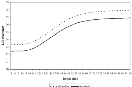
While our calculations are presented in the Appendix, Figures 1 and 2 below summarize our results by showing life expectancy at age 55-59 by income class, for males and females in Flanders and in Wallonia.
Those …gures invite several comments. First, there exists an increasing monotonic relationship between income and life expectancy at age 55-59. That relationship is robust to all genders and regions, and is signi…cant. For instance, a Walloon man in the lowest income class has a life expectancy that is 4 years less than the one of a Walloon man of the highest income group. Second, the income / longevity relationship is non-linear: it is between the second and the sixth deciles that the slope is the largest. But at the two extremes of the income distribution, the income / longevity relationship is less strong. Thirdly, the
com-1 9Poverty rate is the percentage of the population below the poverty threshold …xed at 60%
parison of Figures 1 and 2 suggests that the income / longevity relationship is signi…cantly stronger for men than for women.
In the light of Figures 1 and 2, one can expect that standard poverty mea-sures at high ages are biased downwards. The reasons are twofold.
20 21 22 23 24 25 26 27 28 29 1 4 7 10 13 16 19 22 25 28 31 34 37 40 43 46 49 52 55 58 61 64 67 70 73 76 79 82 85 88 91 94 97100 Income class Li fe exp ect a n cy Flanders Wallonia
Figure 1 : Life expectancy at 55-59 by income class - Male
25 26 27 28 29 30 31 32 33 1 4 7 10 13 16 19 22 25 28 31 34 37 40 43 46 49 52 55 58 61 64 67 70 73 76 79 82 85 88 91 94 97100 Income class Li fe exp ect a n cy Flanders Wallonia
Figure 2 : Life expectancy at 5559 by income class -Female
A …rst reason has to do with the selection mechanism induced by income-di¤erentiated mortality. Given that poor persons tend to live less long than non-poor persons, the poverty rate among the surviving population at age 60 and
more re‡ects not only the "true" poverty, but, also, the interferences associated with the di¤erentiated survival process. That noise tends to reduce the apparent poverty, by the mere absence of the "missing" poor. Hence the poverty rate among Walloon males, equal to 20.4 %, tends, by being based on the population surviving to age 60, to forget the "missing" poor, who faced worse survival conditions than the average because of their poverty.
Besides that measurement problem - i.e. the Mortality Paradox -, one may also argue that a premature death is a part of the poverty phenomenon to be measured. Once it is acknowledged that a Walloon male of the lowest income class lives, on average, 4 years less than one of the highest income class, why should we restrict the measurement of poverty to the income dimension?
Those problems invite distinct adjustments of poverty measures. This sec-tion compares adjusted old-age poverty measures obtained by truncating the income pro…les of the prematurely dead, under various extension techniques.
4.2
General methodology
The adjustment of poverty measures includes two parts. First, the addition of the "missing" poor; second, the imputation of a particular …ctitious income.
Regarding the …rst step, we use the following method. For each income class i and region r = F; W , we have increased the population group Nir on the
basis of the largest life expectancy observed (i.e. the one of top income levels in Flanders). After correction, the adjusted population group is:
^
Nir= Nir
L100F
Lir
where ^Nir is the adjusted population group, Nir is the raw population group,
L100F is the life expectancy of the top income group in Flanders, and Liris the
life expectancy for income group i in region r.
The above computation gives us a new distribution of the population in terms of income, which is the income distribution in the hypothetical case where all individuals had faced the same survival conditions as the ones of a group of reference (top earnings in Flanders). That computation allows us to reintegrate, in our calculations, the missing poor, equal, for each group, to ^Nir Nir.
Under such a computation, the …ctitious income assigned to a prematurely dead individual coincides with his past income. As we discussed above, that ex-tension technique, although attractive, is not the unique possible one. Hence, in the following, we present adjusted poverty measures on the basis of that exten-sion, and contrast these with the ones under alternative extension techniques, including the one relying on the welfare-neutral …ctitious income.20
4.3
Results
Let us …rst consider the simple case where the …ctitious income ei used for the
extension is the one enjoyed when being alive, i.e. yi. For that purpose, we
will proceed in two stages. We will …rst compute the poverty rate for age 60 and more for each gender and region, for the new population computed above,
2 0Throughout this section, the poverty rate is the percentage of the population below the
while assuming that the poverty threshold takes the same level as before the adjustment. Then, we will compute adjusted poverty rates under a new poverty line (taking the modi…cation of the income distribution into account).
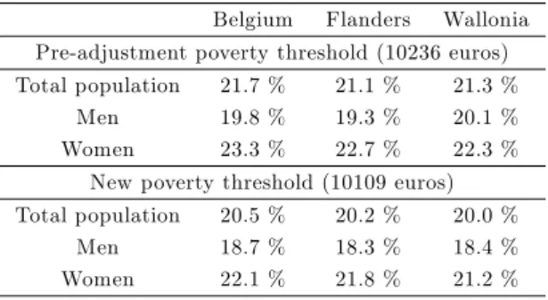
Table 2 shows that, if one keeps the poverty threshold of Table 1, adjusted poverty rates are larger than standard poverty rates. That result is not surpris-ing: our correction, by adding the "missing" persons, consists in adding rela-tively more poor individuals than non-poor individuals. Hence, under a …xed poverty threshold, there must be a rise in the poverty rate. That adjustment is relatively constant across genders and regions, and equal to about 1 point. Such an adjustment, which can be interpreted as the downward bias due to the Mortality Paradox, may be regarded as either low or high. On the one hand, when one considers poverty rates of about 20%, the addition of one point is a minor adjustment. On the other hand, that adjustment looks signi…cant once we think that 1 percent of the population under study consists of thousands of persons and families.
Whereas the …rst part of Table 2 is based on the pre-adjustment poverty threshold, the modi…cation of the population groups in such a way as to neu-tralize the impact of di¤erential mortality has also the e¤ect of changing the income distribution as a whole. Hence, if one adheres to a relativist - rather than absolutist - view of poverty, the addition of "missing" individuals may also a¤ect the level of the poverty threshold. If one computes that new threshold, we obtain a poverty line that is 125 euros lower than the initial one. Under that new threshold, poverty rates tend to fall to levels that are close (if not inferior) to unadjusted poverty rates (second part of Table 2). Thus, if one adheres to a relativist view of poverty, taking the "missing" individuals into account may reduce - rather than raise - poverty.
Table 2: Adjusted poverty rates 60+: …ctitious income = past income Belgium Flanders Wallonia Pre-adjustment poverty threshold (10236 euros) Total population 21.7 % 21.1 % 21.3 %
Men 19.8 % 19.3 % 20.1 % Women 23.3 % 22.7 % 22.3 %
New poverty threshold (10109 euros) Total population 20.5 % 20.2 % 20.0 %
Men 18.7 % 18.3 % 18.4 % Women 22.1 % 21.8 % 21.2 %
Therefore, whether counting the "missing" persons a¤ects the measured poverty or not depends on whether we adhere to an absolutist or a relativistic view of poverty. In the former case, adding the prematurely dead raises poverty. In the latter case, the fall in the poverty threshold is such that the poverty rate is close - if not lower - than before the adjustment. Those results raise the ques-tion of the "right" poverty threshold. We will not address that general issue here, and we will propose poverty measures under the two kinds of threshold.
Whereas Table 2 presupposed that the …ctitious income equals the income when being alive, one can consider other values for that …ctitious income. As dis-cussed above, a natural candidate is the neutral income. That welfare-neutral income is not easy to estimate. As a starting point, we will consider the
case where the welfare-neutral income equals zero, implying that death is, from a welfare perspective, equivalent to a life with zero income.
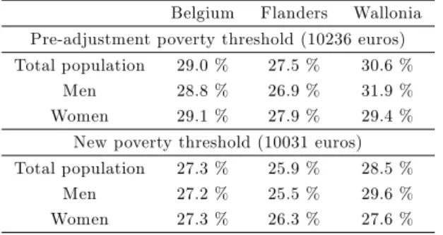
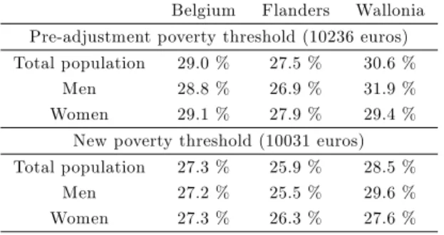
As shown in Table 3, setting the …ctitious income to zero leads to much larger poverty rates, whatever the gender and the region under study. That result is robust to whether we keep a given poverty threshold, or whether we adjust it as a result of the modi…cation of the income distribution. When comparing Table 3 with Table 2, it appears that the adjusted poverty measures are sensitive to the …ctitious income assigned to prematurely dead individuals.21
Table 3: Adjusted poverty rates 60+: …ctitious income = zero Belgium Flanders Wallonia Pre-adjustment poverty threshold (10236 euros) Total population 29.0 % 27.5 % 30.6 %
Men 28.8 % 26.9 % 31.9 % Women 29.1 % 27.9 % 29.4 %
New poverty threshold (10031 euros) Total population 27.3 % 25.9 % 28.5 %
Men 27.2 % 25.5 % 29.6 % Women 27.3 % 26.3 % 27.6 %
Assuming that the welfare-neutral income is equal to zero should only be regarded as a …rst approximation. Actually, the recent literature on the mea-surement of welfare losses induced by premature death allows us to derive more precise estimates of the welfare-neutral income. For that purpose, let us assume, like Becker et al. (2005), that agents have the temporal utility function:
u (yi) =
(yi)1 1=
1 1= +
Following Becker et al. (2005), we …x = 1:25. We estimate the intercept on the basis of the average income in our database, and we obtain: = 15:50. On the basis of those estimates, we obtain a welfare-neutral income equal to 284 euros. Table 4 shows adjusted poverty rates under that …ctitious income.
Adjusted poverty rates under the welfare-neutral …ctitious income are larger than under …ctitious incomes equal to the income when being alive, and, also, larger than unadjusted poverty measures. It is also important to decompose the adjustment into (1) counting the "missing poor"; (2) counting premature death as a part of poverty. The …rst adjustment explains the gap between poverty rates in Tables 1 and 2. That change is small - about 1 point - and not robust to the chosen poverty threshold. The second adjustment explains the poverty di¤erentials between Tables 2 and 4. That di¤erential is large - about 6-7 points - and quite robust to the chosen poverty threshold.
Another important observation to be made concerns the gender poverty gap. In unadjusted terms, Walloon women are poorer than Walloon men (21.6 % against 18.9 %). In adjusted terms, and taking past incomes as a basis for the …ctitious income, women are still more poor than men (22.3 % against 20.1 %). However, once we count premature death as a part of poverty, we obtain
2 1For instance, if one assumes that the …ctitious income equals the past income when being
alive, the poverty rate at age 60 and above lies between 20.5 % and 21.7 %, whereas it lies between 27.3 % and 29.0 % when the …ctitious income is set to zero.
the opposite ranking: Walloon men, because of their worse survival conditions, turn out to be poorer than Walloon women (31.9 % against 29.4 %). Hence, the choice of …ctitious incomes is relevant not only for the description of aggregate outcomes, but, also, for the description of poverty di¤erentials between groups.
Table 4: Adjusted poverty rates 60+: welfare-neutral …ctitious income Belgium Flanders Wallonia
Pre-adjustment poverty threshold (10236 euros) Total population 29.0 % 27.5 % 30.6 %
Men 28.8 % 26.9 % 31.9 % Women 29.1 % 27.9 % 29.4 %
New poverty threshold (10031 euros) Total population 27.3 % 25.9 % 28.5 %
Men 27.2 % 25.5 % 29.6 % Women 27.3 % 26.3 % 27.6 %
5
Conclusions
Under income-di¤erentiated mortality, poverty measures re‡ect not only the "true" poverty, but, also, the interferences due to the survival process. That dependency on survival laws leads to the Mortality Paradox: the worse the survival conditions of the poor are, the lower the measured poverty is.
We proposed to re-examine a solution to that paradox, which consists of truncating lifetime income pro…les, to take the "missing poor" into account. For that purpose, we developed a two-period model with income mobility and income-di¤erentiated mortality. We identi…ed two conditions under which the extension of income pro…les neutralizes the interferences of di¤erential mortality: (1) the …ctitious income is assigned only to the prematurely dead poor; (2) that …ctitious income does not exceed the income when being alive.
Although those conditions are intuitive, these su¤er from two major draw-backs. First, condition (1) is not compatible with the idea that a premature death is a source of poverty for all individuals who face it. Second, condition (2) does not help us a lot regarding the choice of a particular …ctitious income, which is problematic for empirical applications. Therefore, we proposed to extend the adjustment to all prematurely dead persons, and to use, as a …ctitious income, the welfare-neutral income, i.e. the income making an individual indi¤erent between life continuation and death.
Finally, we used regional Belgian data to estimate the size of the Mortality Paradox, as well as the robustness of adjusted poverty measures to the …ctitious incomes used. We showed that the extension of income pro…les by means of …ctitious incomes equal to the incomes when being alive leads to a rise of about 1 point of poverty rate at age 60 and more. But once the poverty threshold is modi…ed to …t the adjusted income distribution, the adjusted poverty rate becomes close to the unadjusted one. We also compute adjusted poverty rates under welfare-neutral …ctitious incomes, and showed that such an alternative adjustment raises poverty rates by about 6 to 7 points. Hence, while the mere addition of the "missing" poor under a constant income leads to a minor varia-tion in the magnitude of poverty, the monetizavaria-tion of premature death by means of the welfare-neutral …ctitious income raises the magnitude of poverty.
In sum, the comparison of standard poverty rates with adjusted ones re-veals that the impact of income-di¤erentiated mortality on the measurement of poverty is far from benign. One should thus be careful when interpreting the levels and variations of usual old-age poverty measures. Those measures hide not only a large number of "missing" poor, but, also, a strong form of depriva-tion: premature death. Thus, two centuries after Malthus’treatise, a particular attention should still be paid to the positive population checks at work in our economies. Otherwise, if we do as if positive checks do not exist, social statistics - including the ones on poverty - will be hardly useful for policy-makers.
6
References
Becker, G.S., Philipson, T. & Soares, R. (2005): "The quantity and the quality of life and the evolution of world inequality", American Economic Review, 95 (1), pp. 277-291.
Bossuyt N, Gadeyne S, Deboosere P, Van Oyen H (2004): "Socio-economic inequalities in healthy expectancy in Belgium", Public Health 118, pp. 3–10.
Broome, J. (2004): Weighing Lives. Oxford University Press: New-York.
Deaton, A. & Paxson, C. (1998): "Aging and inequality in income and health", American Economic Review, 88, pp. 248-253.
Deaton, A. (2003): "Health, inequality and economic development", Journal of Economic Literature, 41, pp. 113-158.
Deboosere, P, Gadeyne, S. & Van Oyen H (2009): “The 1991–2004 Evolution in Life Expectancy by Educational Level in Belgium Based on Linked Census and Population Register Data”, European Journal of Population, 25, pp. 175-196.
Duleep, H.O. (1986): "Measuring the e¤ect of income on adult mortality using longitudinal administrative record data", Journal of Human Resources, 21 (2), pp. 238-251.
Jusiot, F. (2003): "Inégalités sociales de mortalité: e¤et de la pauvreté ou de la richesse", mimeo.
Kanbur, R. & Mukherjee, D. (2007): "Premature mortality and poverty measurement", Bulletin of Economic Research, 59 (4), pp. 339-359.
Malthus, T. (1798): An Essay on the Principle of Population, London.
Mukherjee, D. (2001): "Measuring multidimensional deprivation", Mathematical Social Sciences, 42, pp. 233-251.
Pamuk, E.R. (1985): "Social class inequality in mortality from 1921 to 1972 in England and Wales", Population Studies, 39, 17-31.
Pamuk, E.R. (1988): "Social class inequality in infant mortality in England and Wales from 1921 to 1980", European Journal of Population, 4, pp. 1-21.
Salm, M. (2007): "The e¤ect of pensions on longevity: evidence from Union Army veter-ans", IZA Discussion Paper 2668.
Sen, A. K. (1976): "Poverty: an ordinal approach to measurement", Econometrica, 44, pp. 219-231.
Sen, A.K. (1998): "Mortality as an indicator of economic success and failure", Economic Journal, 108, pp. 1-25.
Snyder, S. & W. Evans (2006): "The e¤ect of income on mortality: evidence from the social security notch", Review of Economics and Statistics, 88 (3), pp. 482-495.
UNDP (1997): The Human Development Report, Oxford University Press: New-York. Van Oyen, H., Bossuyt, N., Deboosere, P., Gadeyne, S., Abatith, E. & Demarest, S. (2005): "Di¤erential inequity in health expectancy by region in Belgium", Social Preventive Medicine, 50 (5), pp. 301-310.
7
Appendix
7.1
Proof of Lemma 1
Let us …rst show that No Mobility Same Poverty implies Robustness to Mortality Changes. For that purpose, take a situation with poverty rate at the young age equal to P1. By the No Mobility Same Poverty condition, we know that, in the
absence of mobility, we have P1 = P2. Take now another situation, with the
same poverty rate at the young age, equal to P10 = P1, but with a worsening
of the survival probability for some income level below the poverty line. By the No Mobility Same Poverty condition, we know that, in the absence of mobility, we have P10= P20. But as P10 = P1, it follows, by transitivity of equality, that
P2= P20 in conformity with Robustness to Mortality Changes.
Let us now prove that Robustness to Mortality Changes implies No Mo-bility Same Poverty. Let us start from a situation where all individuals reach the old age. Assuming the absence of mobility, we get: P2 = P1. Consider now a deterioration of survival conditons for some income group below yP. As
poverty rates at the young age do not depend on survival, we get: P1= P10 (as everything else except the deterioration is left unchanged). Moreover, we have, by Robustness to Mortality Changes, that P20= P2. Hence, by transitivity, we
have P20 = P2 = P1 = P10. Hence, it follows that, in the absence of income
mobility, we have P10= P20, in conformity with No Mobility Same Poverty.
7.2
Proof of Proposition 1
By Lemma 1, we can prove that proposition by merely showing that the old-age poverty rate violates No Mobility Same Poverty. No Mobility Same Poverty requires that, if no mobility, i.e. ii= 1 for all i, poverty at the young age and
at the old age should be the same. In the absence of mobility, P2 is:
P2= PK i=1 in1i PP 1 j=1 ij PK k=1 kn1k = PP 1 i=1 in1i PK k=1 kn1k
Given 1< ::: < K, this cannot be equal to P1, which is given by:
P1= PP 1
i=1 n1i
PK k=1n1k
Actually, in P2, low income group numbers receive lower weights than under
P1 (where the weights are unitary). Hence, it is easy to see that: P2 < P1,
which goes against No Mobility Same Poverty. By Lemma 1, we also know that P2 does not satisfy Robustness to Mortality Changes.
7.3
Proof of Proposition 2
Consider …rst the case where only the initially poor who died prematurely are assigned a …ctitious income. In that case, we have:
If ei < yP for all i: ^ P2= PK i=1 in1i PP 1 j=1 ij +PPi=11(1 i)n1i PK k=1n1k
In the absence of income mobility among those who are alive, this can be rewritten as: ^ P2= PP 1 i=1 in1i + PP 1 i=1 (1 i)n1i PK k=1n1k = P1= PP 1 i=1 n1i PK k=1n1k
Thus No Mobility Same Poverty is satis…ed.
If ei < yP for all i < R P and ei yP for all i R:
^ P2= PK i=1 in1i PP 1 j=1 ij +PR 1i=1 (1 i)n1i PK k=1n1k
In the absence of income mobility, this can be rewritten as: ^ P2= PP 1 i=1 in1i + PR 1 i=1 (1 i)n1i PK k=1n1k < P1= PP 1 i=1 n1i PK k=1n1k
Hence No Mobility Same Poverty is not satis…ed here. If ei yP for all i: ^ P2= PK i=1 in1i PP 1 j=1 ij PK k=1n1k
In the absence of income mobility, this can be rewritten as: ^ P2= PK i=1 in1i PK k=1n1k < P1= PP 1 i=1 n1i PK k=1n1k
Thus the adjusted poverty measure does not satisfy No Mobility Same Poverty.
Let us now consider the case where a …ctitious income level is assigned to all premature dead persons, whatever their past income was. We have the following three cases: If ei < yP for all i: ^ P2= PK i=1 in1i PP 1 j=1 ij +PKi=1(1 i)n1i PK k=1n1k
In the absence of income mobility, this can be rewritten as: ^ P2= PP 1 i=1 in1i + PK i=1(1 i)n1i PK k=1n1k > P1= PP 1 i=1 n1i PK k=1n1k
Thus ^P2> P1, because the premature deaths who used to be rich are now
counted as poor. However, when i! 1 for ei> yP, we have:
^ P2= PP 1 i=1 n1i+ PK k=1n1k + PK i=P(1 i)n1i PK k=1n1k | {z } 0 P1= PP 1 i=1 n1i PK k=1n1k
Hence under a low mortality of the non-poor, the adjusted poverty rate is close to satisfy Non Mobility Same Poverty.
If ei < yP for all i < R P and ei yP for all i R:
^ P2= PK i=1 in1i PP 1 j=1 ij +PR 1i=1 (1 i)n1i PK k=1n1k
Hence without income mobility, we have: ^ P2= PP 1 i=1 in1i + PR 1 i=1 (1 i)n1i PK k=1n1k 7 P1= PP 1 i=1 n1i PK k=1n1k If ei yP for all i: ^ P2= PK i=1 in1i PP 1 j=1 ij PK k=1n1k
Hence without income mobility, we have: ^ P2= PP 1 i=1 in1i PK k=1n1k < P1= PP 1 i=1 n1i PK k=1n1k
Thus No Mobility Same Poverty is not satis…ed.
7.4
Proof of Corollary 1
Indeed, in that case, we have: ^ P2= PK i=1 in1i PP 1 j=1 ij +PPi=11(1 i)n1i PK k=1n1k
Hence, in the absence of income mobility, we have: ^ P2= PP 1 i=1 in1i + PP 1 i=1 (1 i)n1i PK k=1n1k = PP 1 i=1 n1i PK k=1n1k = P1 in conformity with No Mobility Same Poverty.
7.5
Proof of Proposition 3
Under yN < yP, we have: ^ P2= PK i=1 in1i PP 1 j=1 ij +PKi=1(1 i)n1i PK k=1n1kIn the absence of mobility, this can be rewritten as: ^ P2= PP 1 i=1 in1i + PK i=1(1 i)n1i PK k=1n1k = PP 1 i=1 n1i + PK i=P(1 i)n1i PK k=1n1k > P1= PP 1 i=1 n1i PK k=1n1k
Thus ^P2 > P1, because the premature deaths who used to be rich are now counted as poor. Under yN yP, we have: ^ P2= PK i=1 in1i PP 1 j=1 ij PK k=1n1k
Without income mobility, this becomes: ^ P2= PP 1 i=1 in1i PK k=1n1k < P1= PP 1 i=1 n1i PK k=1n1k
7.6
Life tables by income class
There are no lifetable by income in Belgium. However, there exist lifetables by education levels (Deboosere et al, 2009). From these tables, it is possible to estimate lifetables by income class using a weighted ordinary least square regression, as in Bossuyt et al (2004) and Van Oyen et al (2005) studies on health expectancy. Indeed, the position in the social hierarchy is mainly determined by the dimensions: occupation, income and education. Given that the income and education are highly related to one another, we can extrapolate mortality by income class on the basis of the mortality by education. The social position is determined by the educational attainment. A …ve-category classi…cation is used: (1) no formal education; (2) primary education; (3) lower secondary education; (4) higher secondary education; (5) tertiary education. We assume that the position of a socio-economic group is determined by its relative position, de…ned as the mid-point of the proportion of group represents on an ordered scale of 100% (Pamuk, 1985, 1988).
The mortality rates of the educational groups in terms of their relative socio-economic position is estimated using a weighted ordinary least square region of each region and sex and (5-year) age group using aggregate data. The weights are de…ned as the relative sizes of the educational levels in each age group. The slope of the regression line represents the di¤erence in mortality between the bottom and the top of the socio-economic hierarchy. Once estimated, the coe¢ cient is used to compute lifetable according to income by assuming that the social hierarchy is similar to education.
In our case, we used lifetables by age groups of …ve years in order to obtain su¢ cient subsample of each income class. Indeed, we consider one hundred di¤erent groups. Each income class is of 500e except for the highest class which comprehend all income above 50000e.