HAL Id: hal-02411057
https://hal.archives-ouvertes.fr/hal-02411057
Submitted on 15 Dec 2019
HAL is a multi-disciplinary open access
archive for the deposit and dissemination of
sci-entific research documents, whether they are
pub-lished or not. The documents may come from
teaching and research institutions in France or
abroad, or from public or private research centers.
L’archive ouverte pluridisciplinaire HAL, est
destinée au dépôt et à la diffusion de documents
scientifiques de niveau recherche, publiés ou non,
émanant des établissements d’enseignement et de
recherche français ou étrangers, des laboratoires
publics ou privés.
Sodium Fast Reactors
M. Bonney, M. Zabiego
To cite this version:
M. Bonney, M. Zabiego. PIRAT - An analytical tool for reliability assessment of reactivity control
systems - Progress and applications to Sodium Fast Reactors. ICAPP19, May 2019, Juan-Les-Pins,
France. �hal-02411057�
PIRAT - An Analytical Tool for Insertion Reliability Assessment of
Reactivity Control Systems - Progress and Applications to Sodium
Fast Reactors
Matthew Bonney1, Maxime Zabéigo1,*
1CEA Cadarache
CEA/DEN/CAD/DEC/SESC/LECIM 13108 St Paul lez Durance, France
*Corresponding Author : maxime.zabiego@cea.fr
Abstract
Reactivity Control Systems (RCS) are essential safety components for nuclear reactors. One of the most difficult situations these systems experience is seismic motion due to the large deformation and crucial responsibility to shutdown the reactor. This paper introduces a new method for dynamic modeling that accounts for the contact and free motion of the mobile part of the RCS with the guiding sleeve. The new method introduces springs with a gap to account for material interaction. This method is implemented into the DEBSE solver within PIRAT, a toolbox currently in development for RCS design. The work presented in this paper explores the dynamic effects on a model (tentatively representative) system to investigate the assumptions made in some previous works using a quasi-static simulation. Based on the frequency of excitation, various responses are seen that are not captured in the quasi-static simulations. This work gives evidence to the importance of the dynamic modeling of RCS.
KEYWORDS : PIRAT, RCS, Insertion Reliability, SCFR, Seismic Safety
Introduction/Motivation
Reactivity Control Systems (RCS) are critical components for nuclear reactors because they ensure essential safety functions. Operation of the RCS during a seismic event, which is required to achieve reactor shutdown, represents the most challenging situation for RCS design. This is due to the large structural deformations that an earthquake induces, which have the potential of preventing the insertion of the anti-reactivity material into the reactor core. This topic is relevant for a large variety of reactor types, such as: Pressurized Water Reactors (PWR) [1, 2], Boiling Water Reactors (BWR) [3], and Sodium-cooled Fast Reactors (SFR) [4,5,6,7]. There are some slight differences between these reactors when it comes to the RCS systems implemented, but the RCS in general, such as the RBC [7], SCP [5], and CSR [8] systems for SFR-type reactors (as illustrated in Figure 1), are typically composed of:
• A Mobile Part (MP), which embeds the neutron absorbing material into the core during the shutdown process. This is considered a beam-like structure and is typically modeled as a beam with step changes in geometric or material properties [9].
• Two static sleeves that guide the MP during the insertion phase triggered by the seismic activity, as illustrated in Figure 1a. The Upper Sleeve (US) is suspended underneath the Above Core Structure (ACS), while the Lower Sleeve (LS) is supported by the Below Core Structure (BCS) and is surrounded by neighboring fuel assemblies forming a densely packed lattice as pictured in Figure 1b. This lattice increases the stiffness of the LS and is presumable to main drive for deformations imposed onto the MP.
During seismic activities, the induced vibration can cause an issue when inserting the MP by creating a misalignment of the guiding sleeves. Some previous work for this type of analysis was performed by using finite elements and/or some quasi-static representation [3,7,10,11]. The use of finite elements gives the ability to take a design and determine the required force for a mesh point to have an imposed displacement. One issue however is that contact is not always guaranteed at a mesh location or known
a priori. This issue can be relaxed with a high fidelity mesh, but requires a large amount of computational
time, both to create the mesh and to perform the analysis. It is noted that in using the quasi-static representation, both dynamic and static deformations are accounted for. There are static deformations caused by various sources, such as installation misalignment.
The work presented is a study using the computational tool package called Python Implementation for Reliability Assessment Tools (PIRAT) [9]. This package is designed for analytical representation of this
type of system as a time-efficient alternative to finite elements. While finite elements appear suitable for detailed studies at an advanced stage of the RCS design, analytical approaches are judged to be more appropriate for exploratory studies at an early stage of development, since they provide more flexible engineering approaches. PIRAT is developed with two main solvers:
• The Static Bresse Implementation tool (StaBI) is a substitute for a currently used finite element analysis [7], based on the Bresse formulation [12], designed for computing reaction forces (and resulting deformations, contact pressures, etc) induced by static displacements imposed by the sleeves.
• The Dynamic Euler-Bernoulli Implementation for Seismic Events tool (DEBSE) solves the dynamic Euler-Bernoulli equation, designed for producing outputs similar to those of StaBI but as functions of time.
The development of PIRAT has been documented in [9,13]. These show the progress for the components of PIRAT currently with StaBI and DEBSE being developed to a state of usability. The work presented in this paper is a study on the characteristics of dynamic modeling. In particular, this work investigates the validity of the quasi-static assumption that was made in previous work by varying the excitation frequency imposed through the LS and investigating the deflection of the quasi-rigid US. For the true system, the seismic excitation is also active in the ACS and transmitted to the US. If this motion is combined into the excitation of the LS, it is possible to study this excitation through a potential bias that can be corrected in a later stage of the design.
Summary of Numerical Theory
PIRAT is composed on two main solvers, StaBI and DEBSE. Each of these solvers treats the analysis in a different way based on the excitation, static or dynamic. This section gives a general overview of the DEBSE solver and the general framework for the analysis. More detailed explanations on the methods used for both StaBI and DEBSE are presented in [9,13]. Novel to this work, the implementation of DEBSE for non-permanent contacts and non-rigid boundaries is presented here. It is specifically noted that there are other possible implementations for the non-permanent contacts (ex. Hertzian contact model) that will be explored in future work.
For this study, it is assumed that the system of interest is comprised of several sections, therefore the algorithms are based on piece-wise calculations. For DEBSE, this is accounted for by enforcing the deflection, angular displacement, effective moment, and shear force to be continuous across the section transitions. This is enforced through the determination of the natural frequencies and mode shapes. A
(a) Cross-Section View (b) Top View
large portion of the DEBSE calculations occurs in the frequency domain then converted into physical representations to output the results.
Dynamic Theory
The dynamic solver algorithm of DEBSE is complex, but a simplified explanation is presented. To better explain this, Figure 2 shows a simplified MP with two contact locations, 𝑥𝑘for a contact with the rigid sleeve and 𝑥𝑚for a contact with a quasi-rigid sleeve. For the system that is used in this work, the LS is treated as a rigid sleeve with imposed deformation and the US is treated as a quasi-rigid sleeve, where the motion of the sleeve is caused by the motion of the MP (while in a realistic situation, it would also be driven by the motion of the ACS, to be accounted for in future work). This analysis is generalized for any number of contacts for either rigid or quasi-rigid sleeves.
Within DEBSE, the MP is modeled as an Euler-Bernoulli beam with sudden geometric changes [14] with 𝑁𝑘number of rigid sleeve contacts and 𝑁𝑚number of quasi-rigid sleeve contacts. The equation of motion for the transverse displacement 𝑤(𝑥, 𝑡) is expressed as:
𝐸𝐼𝜕4𝜕𝑥𝑤(𝑥,𝑡)4 + 𝑐𝐼𝜕𝜕𝑥5𝑤(𝑥,𝑡)4𝜕𝑡 + 𝜌𝐴𝜕2𝑤(𝑥,𝑡)𝜕𝑡2 = ∑ 𝐹𝑁𝑘 𝑘(𝑡)𝛿(𝑥 − 𝑥𝑘)+ ∑𝑁𝑚𝐹𝑚(𝑡)𝛿(𝑥 − 𝑥𝑚), (1) with c being the Kelvin-Voigt damping coefficient that relates damping to the change in mechanical strain [15], 𝜌𝐴(𝑥) is the linear mass density, 𝐸𝐼 is the structural rigidity, and 𝛿(𝑥 − 𝑎) is the Dirac-Delta function. In this implementation, the Kelvin-Voigt coefficient is not measured in the physical space, but is defined through modal damping coefficients and is expressed as proportional to the Young’s modulus [14].
For the systems of interest, the boundary conditions are not simple. Due to the motion of the sleeves, the ends of the MP are subject to enforced displacement and forces. To account for this, a change of variable is introduced [16] and a modal decomposition is applied as:
𝑤(𝑥, 𝑡) = 𝜙0(𝑡)𝐿−𝑥𝐿 + 𝜙𝐿(𝑡)𝑥𝐿+ ∑ 𝜓𝑁 𝑛(𝑥)𝑞𝑛(𝑡), (2) where 𝜙0(𝑡) and 𝜙𝐿(𝑡) are the displacements at the ends of the MP, 𝜓𝑛(𝑥) and 𝑞𝑛(𝑡) are the mode shapes and modal time histories for mode n. It is noted that selection of the coordinate system origin can remove either 𝜙0(𝑡) or 𝜙𝐿(𝑡) from the analysis. The number of modes kept, 𝑁, is based on the natural frequencies 𝜔𝑛. For this work, the natural frequencies and mode shapes are determined based on simplified boundary conditions, such as pinned-pinned, assuming that the displacement at the ends are accounted for by the change of variable. A detailed explanation of how the frequencies and mode shapes are determined is presented in [13,14] by using the external boundary conditions and the continuity conditions. A Newton-Raphson approach is used on a rank-deficient matrix to determine the natural frequencies, which are then used to calculate the mode shapes.
By applying the change of variable and the orthogonality condition of the mode shapes, Equation 1 becomes a set of modal equations of motion expressed as:
𝑑2𝑞𝑛(𝑡)
𝑑𝑡2 + 2𝜁𝜔𝑛𝑑𝑞𝑑𝑡𝑛(𝑡)+ 𝜔𝑛2𝑞𝑛(𝑡) = ∑ 𝐹𝑁𝑘 𝑘,𝑛(𝑡) − 𝑃𝑛(𝑡) + ∑𝑁𝑚𝐹𝑚,𝑛(𝑡), (3) where 𝜁 is the assigned modal damping, and
𝐹𝑘,𝑛(𝑡) =𝜓𝑛(𝑥𝑘) 𝜌𝐴(𝑥𝑘 ) ⁄
∫ 𝜓0𝐿 𝑛2(𝑥)𝑑𝑥 𝐹𝑘(𝑡) = 𝐶𝑛,𝑘𝐹𝑘(𝑡) (4a) Figure 2: Simplified MP Modeling Schematic
𝑃𝑛(𝑡) = ∫ 𝜓0𝐿 𝑛(𝑥)𝑑𝑥−∫ 𝑥𝜓0𝐿 𝑛(𝑥)𝑑𝑥⁄𝐿 ∫ 𝜓0𝐿 𝑛2(𝑥)𝑑𝑥 𝑑2𝜙0(𝑡) 𝑑𝑡2 + ∫ 𝑥𝜓0𝐿 𝑛(𝑥)𝑑𝑥⁄𝐿 ∫ 𝜓0𝐿 𝑛2(𝑥)𝑑𝑥 𝑑2𝜙𝐿(𝑡) 𝑑𝑡2 = 𝐷𝑛,0𝑑 2𝜙0(𝑡) 𝑑𝑡2 + 𝐷𝑛,𝐿𝑑 2𝜙𝐿(𝑡) 𝑑𝑡2 (4b) 𝐹𝑚,𝑛(𝑡) =𝜓𝑛(𝑥𝑚) 𝜌𝐴(𝑥⁄ 𝑚) ∫ 𝜓0𝐿 𝑛2(𝑥)𝑑𝑥 𝐹𝑚(𝑡) = 𝑆𝑛,𝑚𝐹𝑚(𝑡). (4c)
The solution of Equation 3 can be calculated using a Laplace transform [17] if the forces are known. In this analysis, the displacements are known while the forces are unknown. To account for this, constraints are enforced for each contact location. For the contact locations with the rigid sleeve (LS), this constraint is:
𝑤(𝑥𝑘, 𝑡) = 𝜙0(𝑡)𝐿−𝑥𝐿𝑘+ 𝜙𝐿(𝑡)𝑥𝐿𝑘+ ∑ 𝜓𝑁 𝑛(𝑥𝑘)𝑞𝑛(𝑡)≔ 𝜙𝑘(𝑡), (5) where 𝜙𝑘(𝑡) is the known displacement at the contact location. Further discussion on how this displacement is determined is presented in Section 2.2.
For the contact with the quasi-rigid sleeve (US), more consideration is given due to the coupling between the MP and the sleeve. Because of this interaction, the quasi-rigid sleeve is also modeled as an Euler-Bernoulli beam with a physical equation of motion of:
𝐸𝐼𝑞𝑟𝜕 4𝑣(𝑧,𝑡) 𝜕𝑧4 + 𝑐𝐼𝑞𝑟𝜕 5𝑣(𝑧,𝑡) 𝜕𝑧4𝜕𝑡 + 𝜌𝐴𝑞𝑟𝜕 2𝑣(𝑧,𝑡) 𝜕𝑡2 = − ∑𝑁𝑚𝐹𝑚(𝑡)𝛿(𝑧 − 𝑧𝑚) , (6) where 𝑣(𝑧, 𝑡) is the displacement at location 𝑧 along the beam and the subscript 𝑞𝑟 represent the quasi-rigid beam material properties. It is important to note that the variables 𝑥 and 𝑧 are linearly related. For the quasi-rigid sleeve, it is assumed that the boundary conditions are free-clamped such that the top of the sleeve is clamped into the ACS. In the analysis, the sleeve motion is calculated simultaneously as the MP through a similar calculation (modal decomposition), where𝑣(𝑧, 𝑡) = ∑ ΨΓ 𝛾(𝑧)𝑄𝛾(𝑡). The constraint enforced at the contacts between the MP and quasi-rigid sleeve is:
𝑤(𝑥𝑚, 𝑡) ≔ 𝑣(𝑧𝑚, 𝑡) + Δ𝑚, (7)
where Δ𝑚is a calculated gap to signify contact between the outer edge of the MP and the inner edge of the sleeve. It is also noted that the locations 𝑥𝑚and 𝑧𝑚represent the same physical location.
Through the use of these constraints (Equations 5 & 7), the contact forces can be determined. This is done through an explicit algorithm that utilizes the analytical solution to Equation 3 and a Reimann sum on the convolution integral. Using these techniques, the algorithm results in a linear, matrix expression at each time step. Full details of this algorithm and derivation are presented in [13] when there are only rigid sleeves. For the current implementation (non-permanent contact), the deflections at each contact location is determined via an ODE solver then applied to the system as permanent, rigid contacts. An alternative to [13] is possible for permanent contact with a quasi-rigid sleeve, but is not presented in this paper since it is not used in this current work. This development is documented within an internal report [18].
Implementation
The algorithm presented in this paper makes the assumption that the deflection is known for each time step with permanent contact at each location. This assumption can be valid when comparing the results from a quasi-static loading, but is not necessarily valid when there are dynamic displacements, such as during an earthquake. In order to account for this, an alternative analysis is performed prior to the force determination algorithm. This analysis assumes a functional form of the force magnitude dependent on the dynamic clearance between the MP and the sleeve. Using this form, the equations of motion are integrated to generate the deflection of each contact point. Once this deflection is known, then the previous force algorithm is performed with each location corresponding to a rigid sleeve since the displacement is known at those locations. The coupling effect between the MP and US is accounted for in the implicit differential equation solver.
In order to model the contact, a massless spring with a gap is introduced to represent the contact between the MP and the sleeve. An example of this is shown in Figure 3, where 𝛿𝑘is the gap for the rigid sleeve and 𝛿𝑚is the gap for the quasi-rigid sleeve. These springs take on a unique form similar to
the one presented in [19]. The difference in this formulation for the spring force compared to [19] is based on the expected coating at the contact locations. In production, a layer of coating is applied to the guide regions to reduce frictional effects that might hinder the insertion of the absorber material in the case of shutdown. Due to this layer, the proposed spring force is a two-stage spring, expressed as:
𝐹𝑠 =𝐾𝑐𝑜𝑎𝑡2 (𝑟1+ |𝑟1| + 𝑟2− |𝑟2|) + { 𝐾𝑚𝑎𝑡 2 ((𝑟1− 𝑔𝑘) + |𝑟1− 𝑔𝑘|) 𝑖𝑓 𝑟1≥ 𝑔𝑘 𝐾𝑚𝑎𝑡 2 ((𝑟2+ 𝑔𝑘) − |𝑟2+ 𝑔𝑘|) 𝑖𝑓 𝑟2≤ −𝑔𝑘 0 𝑒𝑙𝑠𝑒 , (8) where 𝑔𝑘 is the thickness of the coating, and 𝑟1 and 𝑟2 are variables that describe the relative displacement of the MP compared to the sleeve.
There is contact if 𝑟1is positive or if 𝑟2is negative referring to if there is contact with the bottom/right part or top/left part of the sleeve (depending on if the system is oriented horizontally or vertically). 𝐾𝑐𝑜𝑎𝑡and 𝐾𝑚𝑎𝑡are spring constants that correspond to the rigidity of the sleeve and coating material. Currently these are specified manually, but future work will investigate to use of a Hertzian contact model as a replacement for the manual specification. Values for these springs are selected based on numerical testing to ensure that there is no large penetration/parasitic contact while considering numerical conditioning on the equations of motion. The definition of 𝑟1and 𝑟2are based on if the contacting sleeve is rigid or quasi-rigid. For a rigid boundary, these are defined for the 𝑘𝑡ℎcontact as:
𝑟1= 𝜙0𝐿−𝑥𝐿𝑘+ 𝜙𝐿𝑥𝐿𝑘+ ∑ 𝜓𝑁 𝑛(𝑥𝑘)𝑞𝑛− 𝜙𝑘− 𝛿𝑘 (9a)
𝑟2= 𝜙0𝐿−𝑥𝐿𝑘+ 𝜙𝐿𝑥𝐿𝑘+ ∑ 𝜓𝑁 𝑛(𝑥𝑘)𝑞𝑛− 𝜙𝑘+ 𝛿𝑘. (9b)
A similar form is given for the quasi-rigid boundary that incorporates the coupling between the MP and sleeve, expressed as:
𝑟1= 𝜙0𝐿−𝑥𝐿𝑚+ 𝜙𝐿𝑥𝐿𝑚+ ∑ 𝜓𝑁 𝑛(𝑥𝑚)𝑞𝑛− ∑ ΨΓ 𝛾(𝑧𝑚)𝑄𝛾− 𝛿𝑚 (10a)
𝑟2= 𝜙0𝐿−𝑥𝐿𝑚+ 𝜙𝐿𝑥𝐿𝑚+ ∑ 𝜓𝑁 𝑛(𝑥𝑚)𝑞𝑛− ∑ ΨΓ 𝛾(𝑧𝑚)𝑄𝛾+ 𝛿𝑚. (10b) With the assumption of this contact model, the modal differential equations are solved via a built-in differential equation integrator within Python. This uses “lsoda” from the FORTRAN library “odepack”. Lsoda is a general wrapper that uses the non-stiff Adams method and the stiff BDF method and contains automatic stiffness detection that selects the best method to use [20]. This solver is used to determine the deflection of all the contact points for every time step. Once these deflections are known, the force determination algorithm is applied with the assumption that all the contacts are with a rigid sleeve. An observation with this methodology is that a contact model is assumed, but then discarded to determine the force values. One important aspect to note, is that the force calculated via the springs gives the relative force between the sleeve and the MP. It does not give the required force to move the sleeve, thus the true force within the MP. Another observation is the required computational time for this analysis. It was found that the differential equation solver did not depend on the specified time step, due to the implicit nature and implementation. This leaves the computational time of the integrator to be very problem dependent primarily for the total length of time to be evaluated. The explicit algorithm on the other hand, is mainly dependent on the number of time steps. However, due to the explicit nature of the algorithm, stability is not guaranteed. In [13], a study was performed on the stability of this algorithm
showing that the general rule-of-thumb used for multiple time steps within the highest frequency tends to produce converged results.
Dynamic Effects
One of the major assumptions used in the quasi-static analysis is that the dynamic effects can be characterized via the maximum deflection of the rigid sleeve. For the quasi-rigid sleeve, a static equilibrium condition is imposed at a guide level. Previous works [7, 9] have shown that for static equilibrium, the maximum displacement of the US is approximately 1 2⁄ → 2 3⁄ of the maximum displacement of the LS and deflects in the same direction representing the motions being in-phase. This work will investigate the relative magnitude observation as well as the in-phase characteristics as functions of the excitation frequency. One important aspect of an actual RCS is that there are multiple sources of deflection, of which some are static and some are dynamic. For previous studies [7, 9], it was found that approximately half of deflection of the LS is caused by the maximum dynamic motion while the rest is based on static misalignment. To investigate the dynamic behavior of the example system considered in this paper, the full deformation (static and dynamic) is modeled as dynamic behavior. Future work will investigate the coupling of the static motion and the dynamic behavior.
Example System
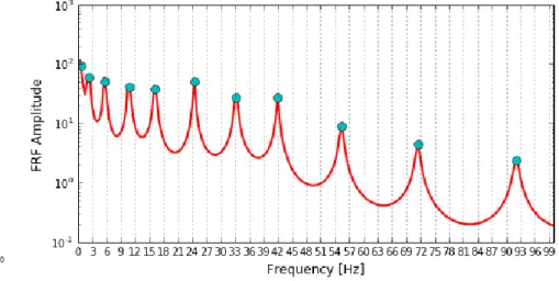
The system of interest for this study in shown in Figure 4a with three main components (LS, MP, and US). This figure shows the region between the BCS and ACS. Additionally, there are three points of interest, the Lower Guide (LG) that is fixed to the bottom-end of the MP, the Intermediate Guide (IG) that corresponds to the guide level of the LS, and the Upper Guide (UG) that corresponds to the guide level at the bottom of the US. Additionally, the frequency response spectrum of the MP with the given boundary conditions is shown in Figure 4b with a smaller damping to better demonstrate the peaks in the amplitude. Additionally, the natural frequencies are also plotted as cyan dots to verify that all the natural frequencies within the range of interest is accounted for. As a note, DEBSE has a built-in feature that allows for manual selection of the natural frequencies. This feature displays the plot in Figure 4b and the user can manually input starting locations for the Newton-Raphson method to determine a new natural frequency or can remove an erroneously determined frequency. The interactive nature and the generation of the frequency response function is optional to reduce computational times.
This model system is designed to be similar to other RCS used in SFR, such as the RBC [7] and SCP [5], but is not associated to any specific reactor. To reflect this notion, this system is called the Model System Configuration (MSC). This contains features similar to the RBC and SCP (three main guide levels, a rigid sleeve and a quasi-rigid sleeve, etc.) but are dimensioned differently for general usability. Preliminary testing was performed in the static regime to compare the MSC to the previously used example system in [9] showing that the systems are similar in deflection profiles and statically determined contact forces, not presented in this work. Specific information about the MSC system is available for collaboration work.
(b) Frequency Response Function with Reduced Damping to Emphasize the Natural Frequencies
(a) Tested Geometry at Specified (Intermediate) Stroke
Dynamic Results and Discussion
The analysis performed in this work assumes that the excitation applied to the MP is through the periodic motion of the LS, which makes contact with the MP at the LG and IG. For this excitation, a single frequency excitation is applied to the LS as compared to a more realistic scenario where a spectrum is applied. By investigating a single frequency, for this preliminary study, the dynamics of the system can be better understood. The frequency of this excitation is variable between 0.4-10 Hz, which is the expected range of frequencies for seimic motion, with a fixed amplitude of around 45 mm displacement at the IG and around 10 mm at the BCS, which is the same amplitude as in [9, 13]. For this work, all displacements are treated as dynamic. It is known that this is not fully representative of a true system, but is used to investigate the properties of the dynamic modeling. Future work will investigate the coupling between the static deformations and the dynamic excitation. Additionally, all the simulations share some common parameters such as: a damping ratio of 5%, time duration of six periods of the sine wave, keeping the natural frequencies below 100 Hz for the truncation of the modal decomposition, and the material and geometric properties of the sleeves and coatings.
There are two main outputs of interest, the deflection of the UG along with the relation of this response to the excitation. The latter is represented by the phase lag between the maximum amplitude of the response and the excitation. The phase lag was chosen because one of the major assumptions made in the quasi-static analysis is that the response and the excitation are in-phase. Although this favorable assumptions makes sense for a static analysis, it is expected that dynamic effects could introduce some phase lag, which would lead to some detrimental shear forces on the MP, with potentially severe consequences on insertion reliability. This lag is calculated based on the time delay of the maximum amplitude of the response and the closest peak on the sine excitation, normalized by the frequency. These two pieces of data are presented in Figure 5. The first important piece of information to gather from Figure 5a is that there is a large increase in the displacement of the UG around 2.2 Hz, as represented by the dynamic amplification factor (measured as the ratio of dynamic amplitude and the quasi-static deflection), which is close to the second natural frequency at 2.29 Hz. This resonance effect will be described and explained in more detail during the discussion of the phase angle. For a physical core, there are limits to the deformation of the UG that is not accounted for in this analysis. Additionally, all the energy of the seismic motion is focused on a single frequency as compared to a realistic excitation that has energy spread across a spectrum. The main take-away from these simulations, in terms of maximum amplitude, is the qualitative result that there is a large increase, nearly twelve times, in the deflection caused by exciting the system near the second natural frequency, possibly caused by the nonlinear nature of this system. Another important piece of information to gather is that away from this
peak, the dynamic amplification factor is near one (red dashed line) while trending to be larger than what is predicted in the quasi-static approach, but within reason. One cause of this might be the slight differences between static and dynamic equilibrium of the beam.
In Figure 5b, the phase lag between the maximum amplitude of the excitation and the response is shown. Within this figure, there are four distinct responses based on the excitation frequency, as marked by the numbered boxes. These different responses are considered to be based on which modes are excited by the motion. A sample of each UG response is presented in Figure 6, with each subfigure representing a different region denoted by <#> to qualitatively demonstrate the activation of different modes due to
Figure 5: Scalar Response Quantities as a Function of Excitation Frequency
the excitation. It is important to note, that at the UG, there is a very tight clearance of a fraction of a mm so the US at the UG level moves almost identically to the MP, which contracts with the IG level where a multi-mm gap exists between the MP and the LS.
In order to fully understand the causes of these responses at the UG, the deformation shape of the MP as a whole is required. One of the possible reasons for the differences in the response is due to the modal activation at various excitation frequencies. In theory, the response is comprised of a linear combination of all the mode shapes of the system with each mode contributing a portion. When the excitation frequency approaches a natural frequency, the contribution of that natural frequency’s mode shape increases. So, the deformation of the system can be used to help determine the frequencies that have a high percentage within the linear combination. Three examples of the full deformation of the MP are presented in Figure 7 for three of the regions noted in Figure 5b. The deformation near the second natural frequency is not shown due to the difference in scale of the deformation, which makes it difficult to express visually.
To illustrate the discussion, the first three mode shapes are presented in Figure 8 with a horizontal line to denote the bottom of the ACS that correspond to the top of the US as shown in Figure 7. The first region of responses is for low frequencies (Figure 6a). This shows a periodic solution with a frequency approximately equal to the excitation frequency and an amplitude close to the amplitude of the excitation at the IG. An excitation of this frequency only seems to excite the fundamental mode (Figure 7a), in which the IG and UG are in-phase. This mode shape can be seen in Figure 8a where the cyan dots represent the UG and IG. For slightly higher frequencies of excitation, the second mode is highly excited. This excitation produces an increase in the amplitude as time progresses as seen in Figure 6b, while also experiencing a phase lag of close to 180◦ meaning that the response is out-of-phase despite the deflections of the second mode both being in phase. Further studies are being performed to investigate the exact cause of this. One possible reason for this increase in amplitude is due to the shape of the second mode (Figure 8b). The excitation at the IG occurs near a maximum point of the shape, causing the response of the system to mathematically divide by a near-zero number. For the other modes, this number is small but not near-zero. Investigating the deflection shape shows the large deformation of the MP, but the motion is not transferred into the US properly represented by large, gross penetration. Further investigation is being performed in order to determine the cause of this increase, if it is a physical situation or a purely numerical issue.
In the third frequency region, the response (Figure 6c) is dominated by the second bending mode as can be seen by the three main peaks occurring at around 2 Hz with some small contribution at the excitation frequency. The displacement at the maximum excitation is seen in Figure 7b. For this excitation, the phase shift of 90◦ is thought to be due to the location of the UG on the mode shape. The
second mode (Figure 8b) has the UG located near the node location, or zero displacement location. This small contribution due the second natural frequency (the primary activated mode) makes the displacement at the UG more sensitive to the deflections caused by the other modes and the motion of the LG. In particular, it is thought that the motion of the LG moves the UG very close to a node location. With the UG being located at a node with zero displacement while the IG is located at a peak, resulting in a phase lag of 90°. The last region produces a multi-modal response (Figure 6d) in which the maximum amplitude can occur either with positive or negative displacement. This region also primarily activates the third bending mode (Figure 8c), as evidence by the deformed geometry in Figure 7c, where the IG and UG are out-of-phase.
One main issue that is brought to light is the difference between these results and the quasi-static analysis. The major differences are the increased magnitude at the UG and the phase based on the excitation frequency. In a true seismic situation, a spectrum of modal amplitudes and frequencies will be applied to the system. This can be thought up as a superposition of individual responses, in which they can amplify or diminish the response of the system due to phase interactions. The work in this paper gives some evidence that an understanding of the dynamic response of the RCS is important for design. It is also important to note that neither of these analyses have been validated to experimental testing. In the past, this type of information was not required due to the use of physical prototypes for qualification purposes. Tests performed on the SCP [5] for instance, did not show any behavior similar to the resonant and out-of-phase tendencies highlighted in this paper. Part of this might be due to the experimental instrumentation and the excitation methodology that is not fully consistent with the methods considered here. Experimental tests are currently being planned to validate the solvers within PIRAT.
Conclusions
This paper was aimed at discussing the development of DEBSE, the dynamic implementation of the PIRAT package dedicated to Reactivity Control System (RCS) insertion reliability studies for nuclear reactors. The emphasis was on presenting the latest modeling that was added to address truly dynamic issues. Prior studies [9] only addressed quasi-static issues. In particular, both MP/sleeve dynamic contacts and semi-rigid sleeves are modeled, which are two critical issues to address within dynamic studies. To demonstrate the development of DEBSE, a preliminary application was discussed, which constitutes a first step on the path to deal with representative systems. This step relies on simplifying hypotheses (continuous beam model), with the purpose of highlighting the potential significance of dynamic effects on the response of a RCS to a seismic event. The characteristics of the considered system are fairly representative of an actual RCS, but the operation conditions are somewhat simplified:
(a) Low Frequency Excitation <1> (b) Resonance Excitation <2>
(c) Mid-Range Frequency Excitation <3> (d) High-Range Frequency Excitation <4> Figure 6: Sample Responses of Upper Guide to Demonstrate Qualitative Differences
Figure 7: Deformed Geometry during Maximum Excitation
• The drop of the MP is not considered. It is maintained at a fixed (adjustable) stroke.
• The excitation is only applied through the LS, with a pure, adjustable frequency. The excitation applied through the US is not taken into account, nor is the excitation spectrum of an actual seismic event.
• Physical limitations that could limit the displacements of the system (other sections of the core) are not fully modeled.
Based on this simplified modeling, the dynamic effects potentially play a key role on the RCS behavior. Compared to static [7] and quasi-static [9] studies, it appears that dynamics effects could produce some detrimental increase to the interactions between the MP and its sleeves. Static studies assume that the two sleeves tend to synchronize their displacements, which favorably enforces the MP through its fundamental bending mode. Taking into account dynamic excitation induces phase-lags that produce increased shear forces on the MP, which are potentially reinforced by resonant behaviors leading to significant dynamic amplification of the deformations, hence impacting insertion reliability.
These observations are not fully understood (at the time of this paper), and part of them could result from numerical artifacts, which are being investigated. However, they represent encouraging preliminary results that will be consolidated and extended in the near future. Experimental validation will be necessary to complement SCP test results [5] that do not seem to address the issues highlighted here.
References
[1] K. Fujita, Y. Shinohara, K. Nanbu, T. Nakatogawa, and T. Nomura. Scram characteristics of control rods of pressurized water reactor under seismic conditions. JSME international journal, 30(267):1450–1457, 1987. [2] B. Collard. Rod cluster control assembly drop kinetics with seismic excitation. In Proceedings of the 11th
international conference on nuclear engineering ICONE 11, Tokyo, Japan, April 2003. ICONE-36419. [3] Y. Koide, M. Nakagawa, N. Fukushi, H. Ishigaki, and Okumura K. Analysis of dynamic insertion of control rod
of BWR under seismic excitation. Journal of Power and Energy Systems, 2(4):1132–1139, 2008.
[4] A. Morrone, A.N. Nahavandi, and W.G. Brussalis. Scram and nonlinear reactor system seismic analysis for a liquid metal fast reactor. Nuclear Engineering and Design, 38(3):555 – 566, 1976.
[5] D. Brochard and P. Buland. Seismic qualification of SPX1 shutdown systems - tests and calculations. In Proceedings of the ICONE-11 Conference, Bologna, Italy, October 1987.
[6] M.N. Sundaran, R. Vijayashree, S. Raghupathy, and P. Puthiyavinayagam. Experimental seismic qualification of diverse safety rod and its drive mechanism of prototype fast breeder reactor. In Proceedings of the FR17 Conference, Yekaterinburg, Russia.
[7] M. Zabiégo, D. Lorenzo, T. Helfer, and E. Guillemin. Insertion reliability studies for the RBC-type control rods in ASTRID. In Proceedings of FR17 Conference, Yekaterinburg, Russia, June 2017. Paper IAEA-NC-254-120. [8] V. Rajan Babu, R. Veerasamy, S. Patri, S. Ignatius Sundar Raj, S.C.S.P. Kumar Krovvidi, S.K. Dash, C. Meikandamurthy, K.K. Rajan, P. Puthiyavinayagam, P. Chellapandi, G. Vaidyanathan, and S.C. Chetal. Testing and qualification of control & safety rod and its drive mechanism of fast breeder reactor. Nuclear Engineering and Design, 240(7):1728 – 1738, 2010.
[9] M.S. Bonney and M. Zabiégo. Validation of PIRAT, a novel tool for beam-like structures subject to seismic induced misalignment of guiding sleeves. In Proceedings of the 2018 International Conference on Noise and Vibration Engineering, Leuven, Belgium, September 2018. Paper #172.
[10] M. Nakagawa and T Jodoi. Insertion analyses of articulated control rods under seismic excitation. In Transactions of the 11th international conference on structural mechanics in reactor technology, 1991.
(a) Fundamental Mode {0.65 Hz} (b) Second Mode {2.29 Hz} (c) Third Mode {5.70 Hz}
[11] S. Onitsuka, H. Ishigaki, Y. Koide, Y. Goto, N. Kawashima, and T. Shiraki. The seismic safety margin evaluation of the BWR scrammability at seismic events. Proceedings of the ICONE-19, the 19th international conference on Nuclear Engineering, 2011.
[12] J. Courbon. Théorie des poutres. Techniques de l’ingénieur, (C2010), 1980. (In French).
[13] M.S. Bonney and M. Zabiégo. Analytic determination of contact force due to dynamically enforced displacements of reactivity control systems in nuclear reactors. Journal of Sound and Vibration, Submitted. [14] M.A. Koplow, A. Bhattacharyya, and B.P. Mann. Closed form solutions for the dynamic response of Euler -
Bernoulli beams with step changes in cross section. Journal of Sound and Vibration, 295(1):214 – 225, 2006. [15] K. Liu and Z. Liu. Exponential decay of energy of the Euler–Bernoulli beam with locally distributed Kelvin–
Voigt damping. SIAM journal on control and optimization, 36(3):1086–1098, 1998.
[16] P.F. Gou and K.K. Panahi. Analytical solution for beam with time-dependent boundary conditions versus response spectrum. In Proceedings of the 9th International Conference on Nuclear Engineering, Nice, France,
April 2001.
[17] D.V. Widder. Laplace Transform (PMS-6). Princeton Legacy Library. Princeton University Press, 2015. [18] M.S. Bonney. DEBSE theory for permanent contacts. Internal Report.
[19] I. R. Praveen Krishna and C. Padmanabhan. Experimental and numerical investigations of impacting cantilever beams part 1: first mode response. Nonlinear Dynamics, 67(3):1985–2000, Feb 2012.