HAL Id: hal-00617902
https://hal.archives-ouvertes.fr/hal-00617902
Submitted on 30 Aug 2011
HAL is a multi-disciplinary open access
archive for the deposit and dissemination of
sci-entific research documents, whether they are
pub-lished or not. The documents may come from
teaching and research institutions in France or
abroad, or from public or private research centers.
L’archive ouverte pluridisciplinaire HAL, est
destinée au dépôt et à la diffusion de documents
scientifiques de niveau recherche, publiés ou non,
émanant des établissements d’enseignement et de
recherche français ou étrangers, des laboratoires
publics ou privés.
Identification of sparse spatio-temporal features in
Evoked Response Potentials
Nisrine Jrad, Marco Congedo
To cite this version:
Nisrine Jrad, Marco Congedo. Identification of sparse spatio-temporal features in Evoked Response
Potentials. ESANN 2011 - 19th European Symposium on Artificial Neural Networks, Computational
Intelligence and Machine Learning, Apr 2011, Bruges, Belgium. pp.447-452. �hal-00617902�
Identification of sparse spatio-temporal features
in Evoked Response Potentials
Nisrine Jrad1, Marco Congedo1 ∗
GIPSA-lab CNRS, Grenoble Univ.
961 rue de la Houille Blanche, 38402 GRENOBLE Cedex, France Abstract. Electroencephalographic Evoked Response Potentials (ERP)s exhibit distinct and individualized spatial and temporal characteristics. Identification of spatio-temporal features improves single-trial classifica-tion performance and allows a better understanding of the underlying physiology. This paper presents a method for analyzing the spatio-temporal characteristics associated with Error related Potentials (ErrP)s. First, a resampling procedure based on Global Field Power (GFP) extracts tem-poral features. Second, a spatially weighted SVM (sw-SVM) is proposed to learn a spatial filter optimizing the classification performance for each temporal feature. Third, the so obtained ensemble of sw-SVM classifiers are combined using a weighted combination of all sw-SVM outputs. Re-sults indicate that inclusion of temporal features provides useful insight regarding the spatio-temporal characteristics of error potentials.
1
Introduction
Many brain computer interfaces (BCI) make use of Electroencephalography (EEG) signals to categorize two or more classes and associate them to sim-ple computer commands. Classification of brain signals is not an easy task because EEG records are high dimensional measurements corrupted by noise. Interestingly, EEG signals often reveal various spatial and temporal characteris-tics. Thus, it is important to characterize both spatial and temporal dynamics of EEG data to provide reliable BCI control.
Usually spatial decomposition is performed to extract the Evoked Response Potential (ERP) components, including Principal Component Analysis, Inde-pendent Component Analysis, etc. These methods define the decomposition in terms of statistical proprieties the components should satisfy in a specific time window. However, ERPs reflect several temporal components, thus, spatial de-composition should be performed for each interesting interval occurring in the pre-fixed window. To this end, some algorithms have been proposed to study where the discriminative information lies into the spatio-temporal plane. They visualize a matrix of separability measures into the spatio-temporal plane of the experimental conditions. The matrix is obtained by computing a separability index for each pair of spatial electrode measurement and time sample. Several measures of separability have been used, for instance the signed-r2-values [1], Fisher score and Student’s t-statistic [5], or the area under the ROC curve [2].
∗This work has been supported through the project OpenViBE2 of the ANR (National
Separability matrix should be sought as to automatically determine intervals with fairly constant spatial patterns and high separability values. This proves difficult and heuristic techniques are often employed to approximate interval bor-ders. In addition, the three first aforementioned measures rely on the assumption that the class distributions are Gaussian, which is seldom verified.
To overcome all these drawbacks, we develop a spatio-temporal data driven decomposition technique without any a priori knowledge or any assumption re-garding EEG dynamics. A two-stage feature extraction technique is proposed. First, a time feature extraction is performed based on Global Field Power (GFP) [3], defined for each time sample as the sum of the square potential across elec-trodes. GFP peaks are associated with maximal signal-to-noise ratio. Second, a spatially weighted SVM (sw-SVM) is proposed to learn for each time interval a sparse spatial filter optimizing directly the classification performance. Finally, the ensemble of sw-SVMs obtained on the selected temporal features are com-bined using a weighted average, to get a robust decision function.
The remainder of this paper is organized as follows. The proposed method is introduced in Section 2. Section 3 accounts for data sets description and discusses the experimental results. Finally, Section 4 holds our conclusions.
2
Method
2.1 Problem description
BCI applications with two classes of action provide a training set of labeled trials from which a decision function is learned. The decision function should correctly classify unlabeled trials. Let us consider an EEG post-stimulus trial recorded over S electrodes in a short time period of T samples as a matrix ˜Xp ∈ RS×T. Hence, the entire available set of data can be denoted {( ˜X1, y1), ..., ( ˜Xp, yp), ..., ( ˜XP, yP)} with yp ∈ {−1, 1} the class labels. Our task consists in finding the spatio-temporal features that maximize discrimination between two classes. 2.2 Temporal features
To select temporal intervals in the ERP where discriminative peaks appear, Global Field Power (GFP) [3] is computed on the difference of the grand averages of the two class post-stimulus trials. Pronounced deflections with large peaks, denoting big dissimilarities between the two activities, are associated with large GFP values. Windows involving significant temporal features are chosen as intervals where GFP is high relative to the background EEG activity.
To select significant windows we require a statistical threshold for the ob-served GFP of the difference grand average trials in the two classes. Such threshold is estimated with a resampling method as the 95th percentile (5% type I error rate) of the appropriate empirical null distribution. For P and Q observed single trials in classes labeled 1 and −1, respectively, we resample P and Q trials with random onset from the entire EEG recording. We compute the difference of the grand average of the P and Q random trials and retain the
maximum value of GFP. The procedure is repeated 1000 times and the sought threshold is the 95th percentile of such max-GPF null distribution after 10% trimming. The trimming makes the estimated GFP more robust with respect to outliers given by eye blinks and other large-amplitude artefacts. Taking the max-GPF at each resampling ensures that the nominal type I error rate is preserved regardless the number of windows that will be declared significant.
Noteworthily, contiguous samples with high GFP coincide with stable deflec-tion configuradeflec-tions where spatial characteristics of the field remains unchanged [3]. Since within each selected time window the spatial pattern is fairly constant, average across time is calculated. Averaging over time rules out aberrant values, reduces signal variability and attenuates noise. Besides, it reduces dramatically time dimensionality to I where I is the number of significant time features. 2.3 Spatial features and classifier : sw-SVM
Temporal filtering provides us with Xp ∈ RS×I trials. Each column vector xp ∈ RS×1 reflects a spatial characteristic at a temporal feature i ∈ {1, ..., I}. Hence, I spatial filters are learned over the different time components. In this work, spatial filtering is learned jointly with a classifier in the theoretical frame-work of SVM. The proposed sw-SVM method (spatially weighted SVM) has the advantage of learning a spatial filter so as to improve separability of classes whilst reducing classification errors. It involves spatial feature weights in the primal SVM optimization problem and tunes these weights as hyper-parameters of SVM. We denote by d ∈ RS×1the spatial filter and D a matrix with d on the diagonal. Matrix D is learned by solving the sw-SVM optimization problem:
min w,b,ξ,D 1 2kwk 2+ C P X p=1 ξp subject to yp(hw, Dxpi + b) ≥ 1 − ξp and ξp ≥ 0 ∀p ∈ {1, . . . , P } and S X s=1 D2 s,s= 1 ∀s ∈ {1, . . . , S} (1)
where w ∈ Rd×1 is the normal vector, b ∈ R is an offset, ξ
p are called slack variables that ensure the problem has a solution in case the data is not linearly-separable, and C is the regularization parameter that controls the trade-off be-tween a low training error and a large margin.
The objective function is not convex with respect to all parameters jointly. Hence, we proceed by alternating the search for a solution of (1). For D fixed, the problem is reduced to a `1 soft margin SVM with the only difference being that xp is replaced by Dxp in the inequality constraint. The primal and dual objective functions of such a problem are convex, and their solution can be obtained by any of the available SVM algorithms. Let us denote by J(D) the optimal value of this problem. By setting to zero the partial derivates of the Lagrangian with respect to the primal variables, the optimization problem of
the dual formulation yielding J(D) can be formulated as follows : J(D) = maxα1Tα−1 2α TYT XTDTDXY α subject to yTα= 0 and 0 ≤ αp≤ C ∀p ∈ {1, . . . , P },
where α is the vector of Lagrangian multipliers, Y = Diag(y1, ..., yn) is the matrix with trial labels on its diagonal, X = {x1, ..., xn} and yT = {y1, ..., yn}.
The value J(D) is thus obtained for a given α by solving the following : min D J(D) subject to S X s=1 D2s,s= 1. (2)
By setting ˜D= DTD, problem (2) reduces to a minimization problem under `1constraints over ˜D. This is clearly an instance of the Multiple Kernel Learning (MKL) problem proposed in [6] with a homogeneous degree 1 polynomial kernel. Authors of [6] prove that the search for the optimal ˜D is convex, yielding fast convergence toward the optimal conditional solution. Hence, the optimization problem can be solved efficiently using a gradient descent as in SimpleMKL [6]. For effect of the `1 constraints, the sought spatial filters will be sparse.
2.4 Ensemble of sw-SVM classifiers
As seen above, a way to reduce EEG variability is to perform signal averaging across time. Another way to reduce this influence, from a classification point of view, is to use an ensemble of classifiers. According to this strategy, a multiple SVM system is designed for each temporal feature. A weighted average on sw-SVM outputs is used to determine a set of significant classifiers. Weights are set as the product of two functions growing proportionally with the accuracies of the two classes (evaluated on a validation set). This weighting strategy is ideal for unbalanced data sets since it seeks classifiers that jointly present good accuracies in both classes. Spatio-temporal features with highest discriminant power are associated with high weights and constitute good candidates for classification.
3
Experimental results
3.1 ErrP data set
The proposed method was evaluated on a visual feedback ErrP [4] experiment. Eight BCI-naif healthy subjects performed the experiment. They had to retain the position of a sequence of digits and to localize where a target digit previously appeared. A visual feedback indicates wether the answer was correct (green feedback) or not (red). Number of digits composing the sequences was adapted with an algorithm tuned to allow around 20% errors for all subjects. Experiment involved 2 sessions that lasted together approximately half an hour. Each session
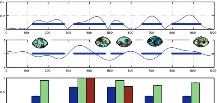
0 100 200 300 400 500 600 700 800 900 1000 0 0.2 0.4 0 100 200 300 400 500 600 700 800 900 1000 −5 0 5 1 2 3 4 5 0 0.5 1
Fig. 1: Top : GFP computed on the difference of the grand average error-minus-correct 1s trials and selected intervals. Middle : the difference computed on electrode FCz and topographies associated with the average in the selected intervals. Bottom : accuracies for error (blue bar) and correct (green bar) classes and sw-SVM associated weights (red bar, normalized between 0 and 1). consisted of 6 blocks of 6 trials, for a total of 72 trials. Recordings of EEG were made from 31 electrodes. Raw EEG potentials were re-referenced to the common average and filtered using a 1 − 10Hz 4th order butterworth filter. A window of 1000ms posterior to the stimulus has been explored for each trial. No artifact rejection was applied and all trials were kept for analysis.
3.2 Results
Single trial classification of error-related potentials is assessed using a 5-Cross Validation technique. Each single training sw-SVM involves a selection proce-dure for setting its regularization parameter C and weights associated to its outputs. Figure 1 shows the average of the difference error-minus-correct for channel FCz of subject 7. It also reports GFP computed on the difference aver-age. Five components are to be noted. A negative deflection can be seen around 240ms after the feedback and a second positive component occurs about 350ms. Three more peaks are also detected; a negative deflection around 500ms, a less pronounced negative deflection around 700ms and a small positive deflection around 800ms. Scalp potentials topographies associated with the 5 extracted temporal features are also shown on Figure 1. The 1st negative peak seems to be occipital whereas the 2nd positive peak covers a rather fronto-central area. The 3rd peak covers a parieto-central area, the 4th peak covers the whole right hemisphere and the last one is more central. Figure 1 shows accuracies for error and correct classes for each sw-SVM and their corresponding weights (normal-ized between 0 and 1). Only sw-SVMs learned on the most pronounced peaks (2nd and 3rd) show good accuracies in both classes and are thus retained.
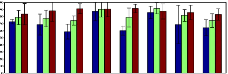
Figure 2 shows the 5 Cross-Validation performance provided by a classi-cal SVM approach where all electrodes are used, the sw-SVM where only one spatial filter was used on the whole trial duration and the proposed method where spatio-temporal features were extracted. The proposed method proved
1 2 3 4 5 6 7 8 0 10 20 30 40 50 60 70 80 90 100
Fig. 2: Performances of classical SVM (Left bar), sw-SVM (Middle bar) and proposed method (Right bar) for the 8 subjects. Mean (std) accuracies across the 8 subjects were 70.71(10.77), 80.71(6.61) and 87.51(3.37) respectively. constantly superior to SVM and sw-SVM. A paired student’s t-test (7 df) was evaluated to compare the proposed method to SVM and sw-SVM and p-values of 0.0044 and 0.0265 were obtained. We conclude that inclusion of temporal features, along with learning an ensemble of classifiers, provide with superior performance.
4
Conclusion
In this paper, a spatio-temporal feature identification was addressed. An analysis of Global Field Power highlighted time periods of interest where effects are likely to be the most robust yielding to a data-driven temporal feature extraction. For each temporal feature, a spatial filter was learned jointly with a classifier in the SVM theoretical framework. Spatial filters were learned to optimize classification performance. A weighted averaging on the so obtained ensemble of classifiers yielded to a robust final decision function. Experimental results on Error-related Potentials data sets illustrate the efficiency of the method from a physiological and a machine learning points of view. These results motivate further research that may aim to extract all relevant aspects of brain post-stimulus dynamics recorded in EEG (spatio-temporal-frequential).
References
[1] B. Blankertz, S.Lemm, M. Treder, S. Haufe, and K. M¨uller. Single-trial analysis and classification of ERP components – a tutorial. NeuroImage, 2010. in press.
[2] M. D. Green and J.A. Swets. Signal detection theory and psychophysics. Krieger, Hunt-ington, NY, 1966.
[3] D. Lehmann and W. Skrandies. Reference-free identification of components of checkerboard-evoked multichannel potential fields. Electroencephalogr Clin Neurophysiol, 48:609–21, 1980.
[4] W. Miltner, C. Braun, and M. Coles. Event-related brain potentials following incorrect feedback in a time-estimation task: Evidence for a generic neural system for error detection. Journal of Cognitive Neuroscience, 9:788–798, 1997.
[5] K. M¨uller, M. Krauledat, G. Dornhege, G. Curio, and B. Blankertz. Machine learning techniques for brain-computer interfaces. Biomed Tech, 49(1):11–22, 2004.
[6] A. Rakotomamonjy, F. Bach, S. Canu, and Y. Grandvalet. SimpleMKL. Journal of Machine Learning Research 9, 2008.