Energy optimization and management of demand response interactions in a smart campus

Article

Energy Optimization and Management of Demand

Response Interactions in a Smart Campus

Antimo Barbato1, Cristiana Bolchini1, Angela Geronazzo1, Elisa Quintarelli1,

Andrei Palamarciuc1, Alessandro Pitì1, Cristina Rottondi2,* and Giacomo Verticale1,*

1 _{Deparment of Electronics, Information, and Bioengineering, Polytechnic University of Milan,} Piazza Leonardo da Vinci 32, Milano 20133, Italy; antimo.barbato@polimi.it (A.B.);

cristiana.bolchini@polimi.it (C.B.); angela.geronazzo@polimi.it (A.G.); elisa.quintarelli@polimi.it (E.Q.); andrei.palamarciuc@mail.polimi.it (A.P.); alessandro.piti@mail.polimi.it (A.P.)

2 _{Dalle Molle Institute for Artificial Intelligence (IDSIA), University of Lugano (USI)—University of Applied} Science and Arts of Southern Switzerland (SUPSI), Manno 6928, Switzerland; cristina.rottondi@supsi.ch * Correspondence: cristina.rottondi@supsi.ch (C.R.); giacomo.verticale@polimi.it (G.V.);

Tel.: +41-058-666-66-72 (C.R.); +39-02-2399-3569 (G.V.); Fax: +39-02-2399-3413 (G.V.) Academic Editor: G.J.M. (Gerard) Smit

Received: 29 March 2016; Accepted: 18 May 2016; Published: 25 May 2016

Abstract: The proposed framework enables innovative power management in smart campuses,

integrating local renewable energy sources, battery banks and controllable loads and supporting Demand Response interactions with the electricity grid operators. The paper describes each system component: the Energy Management System responsible for power usage scheduling, the telecommunication infrastructure in charge of data exchanging and the integrated data repository devoted to information storage. We also discuss the relevant use cases and validate the framework in a few deployed demonstrators.

Keywords:smart grid; smart city; energy management system; renewable energy sources (RESes)

1. Introduction

Making public and private buildings “smart” by integrating innovative Information and Communication Technologies (ICT) in domestic applications is envisioned as a pivotal requirement for a widespread diffusion of local Renewable Energy Sources (RESes), such as solar panels. In turn, the massive adoption of “green” energy sources and their integration in a Smart Grid ecosystem can foster the reduction of carbon emissions and increase efficiency in energy usage. Currently, building heating/conditioning in urban areas account for the largest fraction of the total energy usage [1]. Hence, the application of the concept of Nearly Zero Energy Building (NZEB) [2] plays a fundamental role in the achievement of environmental sustainability objectives.

Several proposals for Energy Management Systems (EMSes) for smart buildings and microgrids have recently been discussed and the implementation details of some demonstrative deployments have been described [3–5]. However, the peculiarities of an academic campus environment require methodological solutions capable of flexibly adapting to different typologies of buildings, according to their specific use (e.g., teaching rooms, laboratories, offices and dormitories), to the presence of controllable loads (e.g., water/heat pumps, Heating, Ventilating and Air Conditioning (HVAC) plants, trigeneration plants and Electric Vehicles (EV) charging points) and of local RESes, possibly in combination with energy storage banks. Decisions about the energy usage schedules must therefore be taken on the basis of prediction models for the energy production patterns of the local RESes (e.g., according to the current weather forecasts) and for the occupancy patterns and rooms temperature of each building (e.g., based on its thermal inertia). Such models rely on weather forecast data and on

real-time data collection from sensor networks deployed within the campus environment to monitor the buildings occupancy and thermal conditions. Moreover, the schedules defined by the campus EMS must adhere to specific comfort constraints in order to guarantee the users’ well-being. To this aim, users are enabled to provide comfort feedback to the EMS via software applications running on portable devices. The EMS must also interact with other actors within the Smart Grid ecosystem (e.g., Distribution and Transmission System Operators, utilities, users, and third party services), support Automatic Demand Response (ADR) in presence of time-variable energy tariffs, and ensure prompt reactions in case of emergencies (e.g., faults in the electricity dispatchment infrastructure). Therefore, a complex telecommunication infrastructure is required to manage the data exchange between the EMS and generators, loads and field sensors/actuators, as well as a data repository infrastructure for information storage and retrieval.

This work presents an energy management framework for a smart campus that encompasses all the above listed functions. Thanks to the flexibility of the proposed solution, such framework can be also adapted to different scenarios (e.g., residential buildings). The framework has been deployed in a set of demonstrators, i.e., office and teaching room buildings in Politecnico di Milano and a private household.

The remainder of the paper is structured as follows: Section2provides an overall view of related work, whereas Section3describes some use cases in which the proposed framework could be adopted. Section4first describes the general framework structure, then focuses on the optimization methods details implemented by the EMS and on the telecommunication infrastructure which manages information exchange, storage and retrieval. The exploitation and assessment of the framework are discussed in Section5. Finally, Section6concludes the paper.

2. Related Work

Several methodologies for the management of energy usage in smart buildings have recently been presented in the scientific literature: reference [6] is a complete survey on the possible approaches. Moreover, frameworks [7–9] provide either real-time or day-ahead energy consumption schedules on the basis of behavioural profiling mechanisms aimed at deducing dwellers habits and at identifying possible energy saving actions. Frameworks integrating local RESes and energy storage banks have also been designed [10,11]. A comparative survey on demand side management systems involving smart buildings and electricity grid can be found in [12].

Focusing on the “Smart Office” scenario, Zarkadis et al. [13] design different algorithms for the control of solar shadings, electric lighting and heating equipment. To this aim, one university building has been extensively monitored through sensor networks for a six years period. Additionally, weather statistics have been recorded. The proposed algorithms led to a consistent reduction in energy consumption without degrading the comfort level perceived by users (and even improving it). Similarly, our proposed EMS includes constraints that guarantee the satisfaction of users’ comfort levels.

Bull et al. [14] evaluate the influence of different engagement strategies on users’ behavior and energy consumption reduction. Balaji et al. [15] include occupants’ feedback into the HVAC management system, transforming the user in an “active sensor” within the building, capable of suggesting improved strategies. To involve users, in our framework we enable interactions between campus occupants and the EMS via a mobile App that allows users to express their perceived comfort level.

Other recent proposals addressing Smart Office environments include energy saving strategies for the management of room lighting based on occupancy detection (by Stojanovic et al. [16]), identification of lighting energy waste patterns in educational institutes by means of data mining techniques [17] and some demonstrative frameworks deploying self-sustained distributed energy systems [3–5,18].

Methodologies for knowledge extraction aimed at automatically inferring and/or updating rule sets for the energy management of a smart office (or a generic smart building) are discussed

by Gupta et al. [19] and Anjos et al. [20]: these algorithms exploit data gathered from smart meters, sensors and actuators installed within the office building and combine them with the users’ preferences in order to define control rules that can be dynamically generated, modified and deleted. However, these rule-inference methods do not guarantee optimality. Other contributions exploit data mining approaches to predict the building energy performance: Fan et al. [21] use ensemble models for predicting next-day energy consumption and peak power, whereas Balac et al. [22] develop a highly scalable framework capable of analysing and predicting the building behaviour considering alternative energy sources and smart grid constraints in real-time.

Among the frameworks specifically tailored for campus environments, Guan et al. [23] design a mixed integer linear model for the joint minimization of gas and electricity expenses of a university building equipped with a controllable combined heat-power system, a battery storage bank and solar panels. The optimization can be performed either relying on forecasting algorithms about future events, or modeling “scenario trees” encompassing multiple possible future production/consumption patterns, which may occur with different probabilities. Our proposed EMS adopts the former approach. However, the optimization procedure is invoked at regular time intervals during the optimization time span and decisions are dynamically updated, following a receding horizon strategy.

In the context of residential buildings, Bozchalui et al. [24] and Kriett et al. [25] propose optimization models for the schedule of domestic electric appliances usage, considering several objectives such as the minimization of the overall energy consumption/expenses, of carbon emissions, and of the peak energy absorption. Our EMS also combines multiple objective functions, including energy expenses, users’ comfort, and the compliance to ADR requests issued by the Distribution System Operator (DSO).

Multiple contributions highlight the importance of the holistic management of building data: Curry et al. [26] exploit linked data as enabling technology to create an integrated graph of relevant knowledge including energy consumption, utility data, occupancy patterns and weather records; Agarwal et al. [27] propose an extensible, distributed and scalable system for storage, shared access and management of building-related information. The prototype facilitates access to the data collected using user management tools and allow standardized client applications to be built on top of it. For the management of relevant knowledge, our solution integrates a data repository devoted to data gathering from different sources (e.g., sensors, actuators, controllable devices) which can guarantee shared real-time access to all the entities within the energy management framework.

The solutions available in literature, both in terms of experimental case studies and approaches, usually tackle a subset of the issues we address in our proposed framework, which offers a scalable solution that integrates a multiplicity of heterogeneous energy sources and loads and directly involves the building occupants.

3. Usage Scenarios

The smart campus may interact with the power grid according to three different paradigms: market-driven, demand response, and emergency. In the market-driven scenario, the amount of power absorbed/injected from/into the grid is autonomously decided by the EMS depending on the current energy price and limited only by the contractual agreements. If such agreements include time-variable tariffs application, tariffs might either be known in advance (e.g., in this case they are computed applying a predefined price curve or according to the day-ahead market) or be dynamically updated with reference to real-time energy market fluctuations.

Conversely, in the demand response scenario, Demand Response Events (DREs) are periodically issued by the DSO. DREs are addressed to one or multiple Points of Delivery (PODs), i.e., electricity subscribers, and include:

• a validity time period; • a monetary incentive;

– an upper bound to the active power that the subscriber can absorb from the grid;

– an upper bound to the active power that the subscriber can inject into the grid;

– an amount of reactive power that the subscriber should inject into the grid.

The DRE is advertised 1.5 h up to one day in advance with respect to the beginning of the validity time period. When a DRE is received, the EMS evaluates different optimization strategies taking into account the DSO request. After the validity time period, the DSO verifies which PODs complied with the DRE requests and applies the monetary discount to the subscriber’s bill.

Lastly, the emergency scenario enables the DSO to control directly the subscriber’s load, bypassing the decisions taken by the EMS. Depending on the emergency condition nature, the DSO might, for instance,

(i) detach the subscriber from the electricity grid; (ii) limit its power injection/absorption; or (iii) modify the amount of injected reactive power.

However, DSO control capabilities of campus loads are much coarser than the EMS ones and the emergency scenario should be considered as an extreme countermeasure, whereas DREs should be applied as a prevention mechanism, in order to shape the campus load consumption curve without upsetting the energy usage schedules independently defined by the EMS.

4. The Energy Management Framework

In this section we introduce the proposed EMS framework by discussing its architecture and internals.

4.1. System Overview

The EMS shares information and activities with a set of actors that contribute to its actions. Among them, the most relevant are:

• Distribution and Transmission System Operators (DSO/TSO), responsible for the electricity dispatchment;

• retail users, equipped with local generation and storage capabilities; • energy utilities, which sell electricity to the retail users;

• energy market, either on real-time or day-ahead basis; • third party services (e.g., weather forecasts providers).

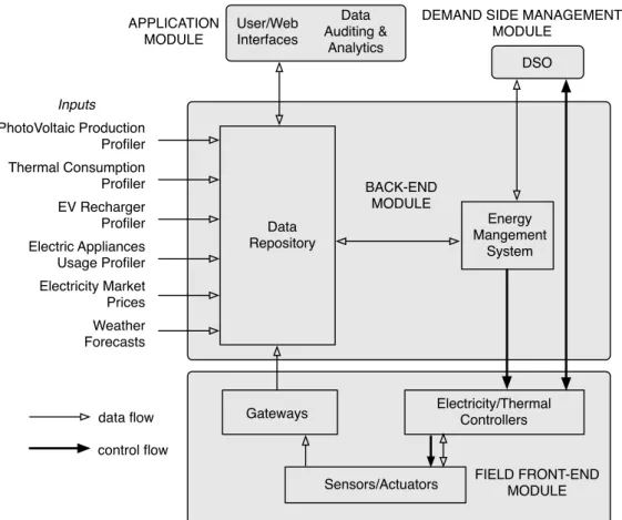
With reference to Figure1, the energy management framework architecture is composed of different modules, which can be also considered as separate domains:

• Demand Side Management Module: consists of the DSO energy management and dispatching infrastructure and its interfaces with TSO;

• Back-End Module: is the core of the framework and comprises the EMS and the data repository. The data repository stores the relevant information shared among the different modules and used by the EMS. The module has a set of interfaces towards the above-mentioned external entities and the repository to collect information, e.g., energy prices provided by energy providers, photovoltaic production and EV usage forecasts provided by profilers, and another set towards the EMS and the application module;

• Front-end Module: includes field sensors and actuators which communicate with gateways and controllers, the latter map the EMS scheduling output into commands to control field devices; • Application Module: merges a set of applications supporting interactions between users and EMS,

including interfaces for users’ preferences setting about their electric appliances management, for the collection of users’ feedback on their comfort level, and for data visualization and monitoring.

PhotoVoltaic Production Profiler Thermal Consumption Profiler EV Recharger Profiler Electric Appliances Usage Profiler Electricity Market Prices Weather Forecasts Data Repository Energy Mangement System DSO User/Web Interfaces Data Auditing & Analytics Inputs BACK-END MODULE

DEMAND SIDE MANAGEMENT MODULE

APPLICATION MODULE

FIELD FRONT-END MODULE Gateways Electricity/Thermal_Controllers

Sensors/Actuators data flow

control flow

Figure 1.The framework architecture.

Users’ comfort feedback is expressed through a mobile App (developed in both iOS and Android) designed following the ANSI/ASHAREE Standard 55-2010. The App allows users to express their perceived comfort with reference to temperature, humidity and air quality.

4.2. The ICT Infrastructure

The ICT infrastructure has been designed to pursue a set of goals:

1. the field devices should work independently from the EMS in case of no provided input; 2. the infrastructure should be flexible enough to accustom multiple adapters comprising a wide

range of field devices;

3. the data collection rate from field devices is independent of the EMS decisions and depends on the specific field device;

4. the EMS takes its decisions evaluating system state snapshots at a given time and available forecasts regarding future energy production/consumption of generators/loads;

5. the EMS chooses one energy production/consumption pattern for each generator/load: the pattern includes power consumption set points for each involved field device within a given time horizon. Field actuators are in charge of translating set points into commands to be issued to devices;

6. the EMS running frequency and optimization horizon might change over time.

On the basis of the stated goals, the ICT infrastructure leverages the two main functional elements in the back-end: the data repository and the EMS. The data repository collects data from the field gateways (which read the field sensors), from the forecast models, and from the EMS (which logs its decisions). Data is available to the EMS, profilers, business intelligence processes and data presentation applications.

The EMS is designed to run at every time slot, but it can be configured to run with a different frequency (e.g., a lower one). The EMS collects the information needed for the optimization from the data repository and executes the optimization algorithm. The optimization output consists of power demand scheduling for passive loads, such as HVACs and EVs, and of storage scheduling for power generated by RESes.

In general, the EMS bases its decisions on predictions which field devices cannot always adhere to. For example, the energy production generated by PV units or power demanded by EVs can be lower than expected. For this reason, the EMS pushes field devices schedules to a group of controllers that transform set points into constraints on the maximum power that each device is allowed to drain from/inject into the system. Prediction errors are prevented in two ways: small errors are handled by running the EMS frequently and by using up-to-date data at each iteration. The EMS continuously updates its decisions to cope with changing conditions and to avoid large accumulated errors, thus limiting inefficiencies. Large errors, such as a completely wrong weather forecast, are dealt by each controller, which can raise the EMS constraints if the controlled field device cannot provide its minimum service. This happens, for example, with the HVACs: when the allocated power results in a too low (or too high) temperature and, consequently, in a too high users’ discomfort, the controller could remove the constraint thus allowing the system to work freely.

The back-end domain comprises the data repository, the EMS and a set of forecast models. The data repository can be hosted either within campus data centers or at any Infrastructure/Platform as a Service (IaaS/PaaS) provider. Back-end components interact with external data sources such as the DSO or the weather forecast service using the Internet, and with the data presentation applications and field front-end by means of the campus LAN.

Gateways and controllers are physical devices equipped with a networking interface, thus enabling communication with sensors and actuators and with the back-end module. Moreover, they are supplied with sufficient computational capabilities to fulfill some predefined automated control operations, such as lifting power constraints if target values can not be met by sensors. Generally, controllers also behave as gateways and interact with the back-end domain.

4.3. The Data Repository

The EMS is able to take educated decisions based on the available information collected during the lifetime of the system and stored in the so-called data repository, depicted in Figure2. In order not to overload the repository with too many data which are not of interest except for the data provider (which would see the repository as a local database) or for the single actor (that would use the repository as a data exchange mean), only information exploited by more than two (sub)systems is stored and shared. In particular, the following pieces of information are stored:

• electricity market prices, collected daily;

• data collected from sensors monitoring the building thermal conditions, energy consumption (within the buildings and from the EV chargers) and the users’ feedback on their thermal comfort, collected with a tunable frequency;

• weather forecasts used to support the estimation of PV energy production as well as the expected energy consumption to heat/cool the building spaces, collected daily;

• EV recharge information, collected dynamically;

• photovoltaic sources energy production, collected dynamically; • accepted DRE manifests;

• energy consumption/production profiles selected by the EMS at each time-slot, providing the on-going strategy actuated by the EMS, collected every time the EMS takes a decision;

• models and technical details for all the elements constituting the system (e.g., building/offices structural information, sensors and actuators datasheets ...).

electricity market price field front-end sensors users' comfort data

cleaning / integration / summarization weather forecast photovoltaic production profiler EMS building thermal controller building electric controller DSO EV controller EV recharge data repository historical energy consumption data controllers' usage/comfort profiles users' aggregated comfort expected PV energy production historical EV usage data analytics

& KPIs UIs

buildings templates & models

requests/incentives

thermal electric profilers

Figure 2.The data repository.

As discussed, these data are used by the EMS to make decisions based on the historical behavior of the system and of the users (e.g., past energy consumption patterns) and on the forecasts of the future demands. In this case, data can be collected with the appropriate frequency (e.g., weather conditions are monitored every 30 min) and periodically pushed to the data repository, since it is not exploited in real-time by any actor, including the EMS. Indeed, there are situations where real-time interaction is needed between two actors (e.g., the EMS and the EV recharge station to interrupt the action in order to immediately reduce energy consumption) and thus direct communication is supported and only the result of the activity is then stored in the data repository.

As a consequence, data in the repository constitutes the system status, updated with a variable delay in the range of tens of minutes. They constitute the source for user applications (such as the one for providing the user comfort feedback), data audit and analysis (also with diagnostic aims), and public displays.

Since data is produced by different (and sometimes redundant) sources, data are integrated, cleaned and summarized, in order to be exploited by the EMS and other controllers. More in detail, a three-layer architecture has been designed for the data repository with the aim of providing a flexible and extensible framework, possibly dealing with different application environments and integrating commercial as well as proprietary data collection solutions.

The lower layer collects raw data from the field (i.e., from wired/wireless sensors, EV recharge stations and energy production/consumption monitors). Gateways have been used to decouple data collection from transmission to the data repository, adopting a polling-based acquisition approach, to manage the high (and possibly variable) number of sensors. This level has been implemented using a NoSQL datastore, Cassandra [28], a distributed database management system designed to handle large amounts of semi-structured heterogeneous data and providing high availability and fault tolerance. A set of distributed algorithms to perform data cleaning and summarization have also been implemented. Furthermore, the system provides online data analysis using an SQL-like query

language and supports batch processing over its distributed file system, thus enabling additional data analytics and KPI evaluations to improve the EMS mission.

The middle layer of the architecture has been implemented with a relational database in PostgreSQL; it is used to store the processed raw data. Data coming from the electricity market, the weather forecast, and DRE manifests are directly stored in this middle layer. As mentioned, together with the dynamic data coming from the various sources, the data repository also stores all the static structured data on the (sub)systems and components characteristics.

The EMS and other controllers/actors access this data through the top layer, which consists in a set of REST APIs, for a coherent access to the information.

4.4. The EMS Interaction Protocol

The core of the EMS is the Optimizer, i.e., an algorithm which chooses the power usage profile of each electric actor that allows the system to minimize the cost function. We now list the parameters taken as input by the Optimizer, which are summarized in Table1.

Table 1.List of main symbols.

Symbol Description Origin

L,G set of power loads and generators System Parameter

Pl set of consumption profiles of load l∈ L lth PG

Pg set of production profiles of generator g∈ G gth PG

ag economic incentive remitted for the usage of generator g∈ G System Parameter T set of time slots within the optimization horizon System Parameter

ft, vt buying and selling energy prices Electricity Market

Et, Vt total absorbed, injected energy scheduled at time slot t Optimizer

D set of active DRE requests DSO

(D =DEmax∪DEmin∪DVmax∪DVmin)

T_d⊂ T set of validity time slots of request d∈ D DSO

DEmax, DEmin set of requests limiting the maximum, minimum power absorption DSO DVmax, DVmin set of requests limiting the maximum, minimum power injection DSO qDEdt

max, qDEdtmin threshold value on maximum, minimum power absorption for each time slot t∈ T_dfor requests d∈DEmax

DSO qDVmaxdt , qDVmindt threshold value on maximum, minimum power injection for each

time slot t∈ T_dfor requests d∈DVmax

DSO

Bd monetary incentive associated to request d∈ D DSO

Et

max, Vmaxt maximum allowed amount of injected/absorbed energy System Parameter qt_{l p} expected average power consumption characterizing profile p∈Plof

load l∈ Lfor each time slot t∈ T

lth PG qt_gp expected average power generation characterizing profile p∈Pgof

generator g∈ Gfor each time slot t∈ T

gth PG ct_{l p} expected comfort level associated to profile p∈Plof load l∈ Lfor

each time slot t∈ T

lth PG cat

l threshold on the minimum comfort level to be guaranteed by load l∈ Lfor each time slot t∈ T

System Parameter Fl p cost (if positive) or gain (if negative) associated to profile p∈Plof

load l∈ L

lth PG Fgp cost (if positive) or gain (if negative) associated to profile p∈Pgof

generator g∈ G

gth PG α, β weights used to control the trade-off between costs and comfort System Parameter α₁, α2 weights used to magnify/reduce the value of the demand response

incentives w.r.t. the energy consumption expenses

System Parameter γt_p weights used to vary the impact of the comfort provided by a specific

load l∈ Lduring a given time interval t∈ T

System Parameter

LetLandG be the set of power loads and generation plants, respectively. Each plant g ∈ G

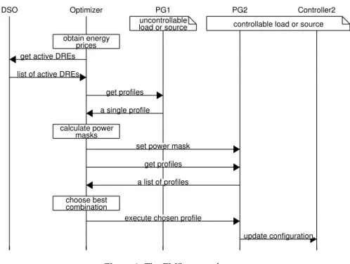
energy. Every electric subsystem (either load or generation plant) is managed by a Profile Generator (PG). Each PG comprises a prediction model of the managed subsystem and is capable of generating several feasible consumption/production profiles. The Optimizer and the PGs operate over a finite scheduling horizon partitioned in a setT of time slots of configurable duration (e.g., for a large campus environment, we consider 15-minute time slots, whereas for a private detached house we consider 5-min intervals). The Optimizer is scheduled to run at the beginning of each time slot and interacts with the other entities according to the protocol in Figure3.

DSO Optimizer PG1 PG2 Controller2

uncontrollable

load or source controllable load or source obtain energy

prices get active DREs list of active DREs

get profiles a single profile calculate power

masks

set power mask get profiles a list of profiles choose best

combination

execute chosen profile

update configuration

Figure 3.The EMS protocol.

First, the Optimizer obtains the time-varying energy prices over the optimization horizon. The prices can be provided by the utility, fetched from the day-ahead market exchange, or predicted in case of participation to the real-time market. At the same time, the Optimizer obtains the list of active DREs. LetDbe the set of DRE manifests the EMS may adhere to. Such requests are associated to a set of time slotsTd⊂ T indicating the request validity time window and to an economic incentive

Bdwhich is remitted to the EMS upon acceptance. The requests are categorized in four subsets:

• DEmax: set of requests d to limit the power absorption below the threshold value qDEmaxdt for each

time slot t∈ Td;

• DEmin: set of requests d to maintain the power absorption above the threshold value qDEdtminfor

each time slot t∈ T_d;

• DEmax: set of requests d to limit the power injection below the threshold value qDVmaxdt for each

time slot t∈ T_d;

• DEmin: set of requests d to maintain the power injection above the threshold value qDVmindt for

each time slot t∈ T_d;

It follows thatD = DEmax∪DEmin∪DVmax∪DVmin. Note that the setsTdare defined over

non-overlapping time windows, i.e., each time slot is included in the validity time span of at most one request. In case no requests are available during a time slot, the maximum amount of injected/absorbed energy is limited by the contractual thresholds Et

max, Vmaxt .

Then, the Optimizer queries the PG of the uncontrollable power loads and generators. These include e.g., lights, elevators, computing equipment, and power sources without energy storage devices. Each of these PGs provides a prediction of the expected energy consumption or generation in each time slot of the optimization horizon.

If the optimization window includes any time slot which falls in a DRE specifying an upper bound for the absorbed power, the Optimizer calculates, for those time slots, the controllable power limit that can be absorbed from the grid by subtracting the uncontrollable power consumption and adding the uncontrollable power generation. Then, the Optimizer executes an algorithm for splitting the controllable power limit into a power limit mask for each PG managing a controllable load (i.e., a manageable appliance whose consumption can be deferred, interrupted and/or tuned). In our implementation, each PG is associated with a predefined weight and the Optimizer simply splits the limit according to these weights. The Optimizer employs a similar algorithm to calculate a power limit mask for PGs managing controllable sources if the optimization windows contains DREs specifying an upper bound to the injected power.

Next, the Optimizer sends to each controllable PG the power limit mask and queries for a set of profiles over the optimization horizon. Each PG must propose one or more feasible profiles corresponding to different comfort levels and different energy consumption or generation schedules. In case the EMS advertises a power limit, then the PGs should also propose profiles that satisfy the limit in addition to the usual profiles, so that the EMS can decide whether to comply to the DRE requests. The strategy used to elaborate the proposal is PG-specific and depends on the available field data and available models. In general, each PG should be able to provide at least one backup profile, which might be suboptimal.

The separation between Optimizer and PGs makes it possible to cope with time-varying, non-linear constraints without jeopardizing the manageability of the linear optimization model. For example a storage system might have constraints with respect to the number of daily charge/discharge cycles. This can be easily implemented in the PG for the storage system, which proposes only solutions with a duty cycle compatible with the expected battery aging. In turn, the optimizer is bound to choose one of the proposed profiles.

Each power load (generation plant) is then characterized by a set of power consumption/production profiles Pl∀l ∈ L(Pg∀g∈ G). Note that the optimization algorithm of the

EMS is agnostic w.r.t. the criteria the profile generation process is based on. Such criteria may take into account several factors such as the weather forecasts, the trend of the electricity prices, and the users’ preferences. Each generated profile comprises:

• a unique ID;

• a list of set points and their corresponding time schedule to enforce the system to behave according to the profile shape;

• a 24-h profile qt

l p(qtgp), indicating the expected average power consumption or generation for

each time slot t∈ T; • a 24-h profile ct

l pof the expected comfort for each time slot (this profile may represent thermal

comfort, or the satisfaction of the users of the electric vehicles: the exact semantic depends on the specific PG); a threshold cat_lon the minimum comfort level that each load must ensure for every time slot is also included.

• a gain or cost Fl p (Fgp) associated to the profile, which may take into account the usage of

non-electric power sources such as gas for heating, the exploitation of economic incentives for using RESes, or different wear and tear costs. Gains are expressed with negative values, whereas costs are expressed with positive values.

Once all the queried PGs provide their list, the Optimizer chooses the best combination of profiles by means of the algorithm described in Section4.5and sends the chosen profile ID back to each PG. Each PG is then responsible of enforcing the chosen profile by configuring the relevant controllers so that the field devices behave as desired.

It is worth noting that controllers are configured for an entire optimization horizon, but the configuration can be overwritten at each optimization time slot if external conditions change, (e.g., better predictions are available or new DRE is published by the DSO).

4.5. The EMS Optimization Model

Whenever a new time slot starts, the EMS receives the energy production/consumption profiles generated by the PGs and the energy buying/selling prices ft, vt ∀t ∈ T. The EMS then runs the

following Mixed Integer Linear Programming (MILP) model to schedule the energy usage plan over the horizonT.

4.5.1. Variables

• Et(Vt): non-negative variables, indicate the total absorbed/injected energy during time slot t; • yl p(ygp): boolean variables, set to 1 if profile p ∈ Pl(p ∈ Pg)is chosen for plant l ∈ L(g ∈ G),

0 otherwise;

• γt_E (γt_V): boolean variables, set 1 if some energy is absorbed (injected) during time slot t,

0 otherwise;

• wdt: boolean variable, it is 1 if request d∈ Dis satisfied during time slot t, 0 otherwise; • zd: boolean variable, it is 1 if request d∈ Dis satisfied in every time slot t∈ T, 0 otherwise.

4.5.2. Objective Function

The goal of the EMS is to decide which power production/consumption profile each load/generator must follow over the horizonT with the aim of minimizing the total energy expenses while maximizing the users’ utility. To this end, the objective function is modelled as follows:

min    α  α1  

∑

∑

∑

∑

∑

∑

∑

∑

∑

∑

∑

∑

where the first contribution represents the total cost incurred by the system, obtained as the difference between the daily energy expenses and the economical incentives remitted through ADR, whereas the second contribution represents the comfort of users. The coefficients α and β are weights used to control the trade-off between costs and comfort. Two additional weights α1, α2are used to magnify/reduce

the value of the demand response incentives w.r.t. the energy consumption expenses. Similarly, the coefficients γt_pare used to vary the impact of the comfort provided by a specific load l during a given time interval t.

4.5.3. Constraints

Constraints2and3impose that only one profile is chosen for each load/generator. The energy balance of the system in each time slot is ensured by Constraint4, whereas Constraints5and6maintain the energy absorption/injection within the contractual limits. Moreover, Constraint7imposes that the system either absorbs power from the grid or injects power into the grid (i.e., the unidirectionality of the power flow) during each time slot. Constraint8ensures that the comfort level provided by each does not drop below a minimum acceptability level. The final group of equations imposes the compliance to the demand response requests (in case they are accepted), according to their type: Constraint9limits the power absorption below the threshold qDEdtmax; Constraint10maintains the power absorption

above the threshold qDE_mindt ; Constraint11limits the power injection below the threshold qDVmaxdt ;

Constraint12 maintains the power injection above the threshold qDV_mindt ; Constraint 13 imposes that the above mentioned limitations are activated for the whole validity time span of the demand response requests.

∑

p∈P_l

∑

∑

∑

∑

∑

∑

Et≤qDEdtmaxwdt+Etmax(1−wdt) ∀d∈DEmax, t∈ Td⊂ T (9)

Et≥qDE_mindt wdt ∀d∈DEmax, t∈ Td⊂ T (10)

Vt≤qDV_maxdt wdt+V_maxt (1−wdt) ∀d∈DVmax, t∈ Td⊂ T (11)

Vt≥qDV_mindt wdt ∀d∈DVmax, t∈ Td⊂ T (12)

∑

t∈Td⊂T

wdt≥zd|T_d| ∀d∈ D (13)

5. Framework Validation

A pilot version of the proposed framework has been implemented and is currently in service at the Politecnico di Milano Campus to manage the controllable production, storage, and loads of a large building. The building comprises four floors used for various university activities. Roughly classrooms make up 60% of the building, whereas 15% is occupied by classrooms equipped with electric plugs available to students and the remaining 25% by administrative offices. The building frame is mainly composed of reinforced concrete while the external walls are composed by glass and reinforced concrete with insulating material in between. Double layer strip windows surround all the building. The gross floor area is equal to 3,344 m2, requiring 58 kWh/m3per year for heating. The building operates in grid-connected mode, so any mismatch between consumption and production results in a power exchange with the grid different than expected and, consequently, in a suboptimal usage of resources. The electric actors serving the building are three:

1. Photovoltaic system. The photovoltaic plant is an integrated rooftop solution capable of

supplying both electric and thermal energy. The maximum electric power reached in standard conditions is 10 kW with an electric efficiency of 15.06%, while the thermal contribution can reach 1,040 W at 80℃. The plant receives incentives for production, therefore ag=0.35e/kWh.

Currently, the PG associated to the PV plant is very simple and only considers hourly and seasonal variations. The design of a more sophisticated predictor that considers both weather forecast [29] and short term dynamics [30] is left for future work.

2. Heating, Ventilating and Air Conditioning system (HVAC). Two heat pumps are used for

heating and cooling. The first one can supply up to 374 kW of cooling power and up to 429 kW of heating power (ESEER 5.65, COP 4.1) for an overall maximum electric consumption of 82.4 kW. The second one can supply a cooling power up to 114 kW, heating power up to 110 kW and is characterized by a maximum electric consumption equal to 21.4 kW. For what concerns the air distribution system, two collectors receive the carrier coming from the heat pumps and feed the air handling units (AHUs) and all the fan coils of the building. Moreover, a 23 m3thermal storage has been installed exploiting the fire system tank which can be used during the summer season. Set points can be automatically imposed thanks to a Supervisory Control and Data Acquisition (SCADA). The building also comprises a natural gas boiler as a backup for the HVACs. In case it

is necessary to turn on the boiler to achieve a desired comfort level, the PG will provide a profile with nonzero Flpt.

3. Electric Vehicles recharge system. The building includes a recharging station that can supply

up to 20 kW to a connected electric vehicle. Testing was conducted using a Renault Zoe with a battery capacity of 22 kWh. This car model accepts variable AC input power from 9 kW up to 43 kW, allowing for quick recharge in less than one hour. The supported variable input power is crucial for the energy scheduling defined by the EMS.

Overall, the demonstrator has a maximum power supply equal to 200 kW and can feed the network up to 10 kW depending on the photovoltaic energy available. For each electric actor we implemented a suitable Profile Generator (PG), so G = {PV system} and

L = {HVAC, EV, uncontrollable loads}, where the third element of the set groups all the

non-controllable appliances. In the experimental setup, each hour the EMS uses the protocol described in Section 4.4to collect from each PG the set of proposed profiles and runs the MILP model described in Section 4.5to choose the optimal combination, which is then delivered to the actuators. The environmental and thermal data are sampled and stored every 6 min. HVACs, EV recharge stations and building loads energy consumption are collected with a 1-minute frequency. Sensed data are stored locally on the ICT infrastructure gateways, and pushed to the data repository every 15 min. These parameters provided a good trade-off between access frequency to the data repository and amount of stored data.

In this section, we briefly report on the collected data and discuss how the exploitation of the framework allows for a modulation of the energy consumption.

5.1. Preliminary Analysis of the Collected Data

A preliminary analysis has been performed to compare the comfort level perceived and reported by the occupants by means of the mobile App, and the comfort level that can be inferred from the sensor data by applying the classification defined by the Italian national regulation. The App has been designed following the ANSI/ASHAREE Standard 55-2010 that recommends a 5-labels scale to survey users’ opinion, as summarized in Table2. In particular, the purpose of our work is to get useful insights on specific scenarios that require marked attention by the EMS. Our preliminary analysis stresses the urgency of adopting an intelligent system able to smooth critical recurrent scenarios, e.g., remarkable changes in weather conditions, and to adopt long-term smart strategies, e.g., improving the management during non-working days. Indeed, the aim of the optimization algorithm is twofold: improving the comfort perceived by occupants while possibly reducing the energy consumption due to HVACs.

Table 2.Comfort feedback scale.

Vote Perceived Temperature

−2 too cold

−1 cold

0 comfortable

1 hot

2 too hot

Since April 2015, we have been monitoring a sets of variables inside and outside a group of university buildings: in each building we gather data regarding temperature, humidity, lightness and air quality on a selected subset of rooms. We further record data from the weather station installed on the rooftop of one block which includes air temperature, relative humidity, pressure, etc. The buildings are close enough to use a single weather station to monitor weather conditions. The analysis has been carried on in a market driven scenario as previously detailed in Section3.

For the sake of conciseness, we report data collected in the building where the EMS is installed during one summer month and one winter month. In both periods the HVAC system is turned on.

The following analysis focuses on temperature, as the main factor influencing the comfort perceived by the occupants. We examined the data collected during the first phase of our experimentation with reference to the current Italian national regulation ISO 7730/2005, briefly summarized in Table3. Each class corresponds to an operative temperature interval in winter and summer time, and the last column provides the Predicted Percentage of Dissatisfied occupants (PPD). Winter and summer times are discriminated according to the external average daily air temperature; if the temperature exceeds 15°C, the summer case should be applied.

Table 3.Comfort classes defined by the Italian national regulation ISO 7730/2005.

Class Summer Winter PPD

A 24.5℃±1.0℃ 22.0 ℃±1.0℃ <6% B 24.5℃±1.5℃ 22.0 ℃±2.0℃ <10% C 24.5℃±2.5℃ 22.0 ℃±3.0℃ <15%

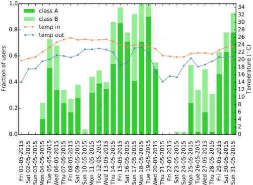
Results have been computed assuming that the operative temperature is approximated by the sensed air temperature. The temperature has been calculated by averaging the data collected by all the temperature sensors installed inside the building, within 15 min, during working hours (i.e., from 8 am to 6 pm). More sophisticated techniques, such as mode or median, introduce complexity considering the high number of sensors and the short sampling time, while carrying little benefit to this approximate analysis. The charts in Figures 4and 5 depict the disjointed percentage of temperatures falling within class A and B, i.e., classes with dissatisfied users percentages below 6% and 10%, respectively. In addition, internal and external average daily temperatures are plotted on the secondary vertical axis to offer a deeper understanding. It is worth noting that days with no plotted percentages show average temperatures falling out of the ranges of classes A and B, thus highlighting high discomfort or high energy waste due to overcooling or overheating.

Indeed, the worst results occurred in presence of a steep change in the outside temperature: this suggests that the EMS needs to improve its strategies during these days. As it can be noted in Figures4and5, in the last part of May, after the sudden temperature decrease from 21.7°C to 14.6 °C within two days, the user comfort decreases. A similar pattern can be identified during the first week of November, when the building was overheated to 27°C to counteract the sharp decrease of the outside temperature. In brief, the system needs better tuning with reference to the weather forecast, to provide an appropriate comfort to the occupants while saving energy, e.g., to avoid overheating.

A further point to consider concerns non-working days when the comfort goal is neglected by the EMS, being the building supposedly empty. This means setting the comfort level to be ensured to its minimum, thus allowing the EMS to maximize other goals. During these days (e.g., from 1 to 3 May, 23–24 May and 21–22 November), the inside temperature is more closely related to external conditions and to the other objectives considered by the EMS (e.g., cost and power consumption), indeed on holidays and weekends the objective is to maintain a certain temperature in order to avoid a greater effort on HVAC restarting.

Tables4and5show the percentage of users in each comfort class measured (a) through the mobile App feedback or (b) inferred by applying the ISO regulation in the same instant when a user reported a feedback and considering comfort classes disjointedly. Summer period comprises May, June, July and September while winter period includes November, December, January and February. The analysis of the comfort feedback collected through the mobile App shows that satisfied users are around 50% in each period. On the other hand, very dissatisfied users, i.e., users who vote−2 or 2, range between 15% and 30%. In each period the results are consistent since class A contains the highest percentage of comfortable users, as pointed out by the gathered feedback.

Fri 01-05-2015 Sat 02-05-2015 Sun 03-05-2015 Mon 04-05-2015 Tue 05-05-2015 Wed 06-05-2015 Thu 07-05-2015 Fri 08-05-2015 Sat 09-05-2015 Sun 10-05-2015 Mon 11-05-2015 Tue 12-05-2015 Wed 13-05-2015 Thu 14-05-2015 Fri 15-05-2015 Sat 16-05-2015 Sun 17-05-2015 Mon 18-05-2015 Tue 19-05-2015 Wed 20-05-2015 Thu 21-05-2015 Fri 22-05-2015 Sat 23-05-2015 Sun 24-05-2015 Mon 25-05-2015 Tue 26-05-2015 Wed 27-05-2015 Thu 28-05-2015 Fri 29-05-2015 Sat 30-05-2015 Sun 31-05-2015

0.0

0.2

0.4

0.6

0.8

1.0

Fraction of users

class A

class B

temp in

temp out

0

2

4

6

8

10

12

14

16

18

20

22

24

26

28

30

32

34

Te

m

pe

ra

tu

re

(

C)

Figure 4.Comfort analysis w.r.t. ISO 7730/2005 May 2015, comfort classes daily percentage plotted on the main vertical axis.

Sun 01-11-2015 Mon 02-11-2015 Tue 03-11-2015 Wed 04-11-2015 Thu 05-11-2015 Fri 06-11-2015 Sat 07-11-2015 Sun 08-11-2015 Mon 09-11-2015 Tue 10-11-2015 Wed 11-11-2015 Thu 12-11-2015 Fri 13-11-2015 Sat 14-11-2015 Sun 15-11-2015 Mon 16-11-2015 Tue 17-11-2015 Wed 18-11-2015 Thu 19-11-2015 Fri 20-11-2015 Sat 21-11-2015 Sun 22-11-2015 Mon 23-11-2015 Tue 24-11-2015 Wed 25-11-2015 Thu 26-11-2015 Fri 27-11-2015 Sat 28-11-2015 Sun 29-11-2015 Mon 30-11-2015

0.0

0.2

0.4

0.6

0.8

1.0

Fraction of users

class A

class B

temp in

temp out

0

2

4

6

8

10

12

14

16

18

20

22

24

26

28

30

32

34

Te

m

pe

ra

tu

re

(

C)

Figure 5. Comfort analysis w.r.t. ISO 7730/2005 November 2015, comfort classes daily percentage plotted on the main vertical axis.

Table 4. Comfort analysis summer 2015. (a) Feedback collected through the mobile App; (b) ISO 7730/2005 comfort class. (a) Class Samples (%) −2 8 −1 17 0 49 1 20 2 6 (b) Class Samples (%) A 56 B 19 other 25

Table 5. Comfort analysis winter 2015. (a) Feedback collected through the mobile App. (b) ISO 7730/2005 comfort class. (a) Class Samples (%) −2 18 −1 16 0 43 1 12 2 11 (b) Class Samples (%) A 32 B 22 other 46

5.2. Energy Scheduling in the Demand-Response Scenario

In the Demand-Response scenario, the DSO can send DREs to the low voltage and medium voltage customers in presence of issues related to the energy dispatchment within the distribution network (e.g., overloads). Every hour, the EMS checks the presence of new requests. If one or more DREs are found, it includes them in the setD. If the incentive offered in the DRE manifest compensates the efforts for a rescheduling, the EMS may alter the load profiles of the electric actors during the subsequent 24 h.

We show how the system reacts to DRE events by comparing the EMS schedule in a typical day without DREs versus the schedule obtained in presence of a DRE event. For this experiment, the MILP formulation proposed in Section4.5has been implemented and solved with the AMPL-CPLEX solver. We set the cost-comfort tradeoff coefficients α, α1, and α2equal to 1. This means that a euro saved by

shifting a load or a euro gained by satisfying a DRE event are equivalent. Therefore, assuming two possible schedules result in the same comfort level, the EMS will reschedule a load whenever the DRE incentive will, at least, cover any additional cost. The coefficients γt_pare set to 1/24 so that the daily comfort for each PG is the average comfort in each time slot and ranges from 0 to 1. The coefficient β is set toe 20, which means that the optimizer chooses to reduce the daily comfort by 10% if it results in saving 2 euros. This value is intentionally high. With typical energy prices, it impossible for the optimizer to decide to simply reduce the comfort in order to save money. In normal conditions, the EMS will try to provide the maximum comfort at the minimum cost. On the other hand, the EMS could reduce the comfort if a DRE incentive is large enough to make up for the comfort loss. In all the considered instances, the computational time was in the order of a few seconds.

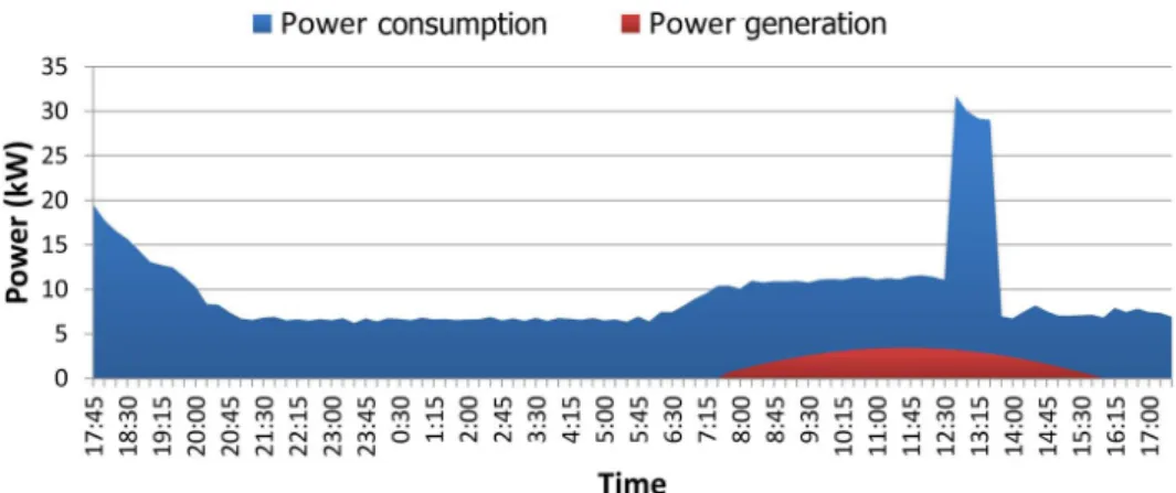
Figure6shows the power consumption scheduled by the EMS at 17:45 by considering the expected production of the PV plant (red curve) and the sum of the expected consumption of the uncontrollable appliances, the HVACs and the EV recharge stations. It is worth noting that, at the time the optimizer is executed, the HVAC is going off and it is not scheduled to run on the following day.

Figure 6.Average Power Schedule Et/(1 h)and Vt/(1 h)during the test day in absence of DREs.

When no DRE manifest is present, the decision only depends on the energy prices, which are shown in Figure7. The power consumption spikes at 12:30 is due to recharge of the EV. In this experiment the EV was scheduled to be available during office hours and the EMS schedules its recharge when the energy prices are at their lowest within such time interval.

Figure 7.Energy prices ftand vtduring the test day.

At 18.30, the EMS downloads a new DRE manifest, sets the new threshold in the constraints of the optimization model and invokes the Optimizer. The simulated DRE event sets a power absorption cap from the grid at 10 kW between 10:45 and 15:15, with a reward equal to 1 euro.

As reported in Figure8, the results of the new optimization shift the EV recharge schedule of a few hours in advance with respect to the previous configuration because, when taking the incentive into account, the new schedule becomes cheaper. This choice of the EMS heavily depends on the incentive amount. If the incentive is low, the EMS will not alter the consumption schedule of the campus.

If the incentive is too high, the EMS might lower the campus users’ comfort level in order to fulfill the DRE. In turn, this could increase the number of unsatisfied occupants. We plan to study the impact of different incentives on the discomfort and on the willingness to experiment discomfort in exchange for a lower probability of emergency actions. The goal is to provide data to the DSO regarding the effectiveness of a DSO-driven incentive-based policy to increase system availability.

consumption generation

Figure 8.Average Power Schedule Et/(1 h)and Vt/(1 h)during the test day in presence of one DRE.

6. Conclusions

This paper proposes an energy management framework for a smart campus including local renewable energy sources, a storage bank, and several controllable loads. The framework incorporates an optimizer which schedules the usage of electric loads, various predictors for the energy production/consumption patterns, a repository and an ICT infrastructure dedicated to data collection and management. The paper discusses relevant use cases and evaluates the performance of the proposed framework.

In the market-driven scenario, the EMS minimizes the cost of energy by, among others, fostering self-consumption. On the other hand, the impact on the comfort and the total energy consumption is minimal.

In the DSO-driven scenario, the EMS reacts to DSO requests by modifying and rescheduling energy consumption and/or production depending on the associated incentive. This is an entirely new scenario enabled by the EMS that results in an economic advantage for the final user. The monetary impact depends on the amount of incentives that are provided by the DSO, which is still under study.

Acknowledgments: The work in this paper has been partially funded by Regione Lombardia under grant no. 40545387 Smart Campus as Urban Open LAbs (SCUOLA).

Author Contributions: Antimo Barbato and Cristina Rottondi equally contributed to the the design of the EMS optimization algorithm. Andrei Palamarciuc, Alessandro Pitì, and Giacomo Verticale equally contributed to the design and implementation of the back-end module, the DR protocol, and the EV profile generator. Cristiana Bolchini, Angela Geronazzo and Elisa Quintarelli equally contributed to the the design and implementation of the data repository, the application module and part of the field front-field module.

Conflicts of Interest:The authors declare no conflict of interest.

Abbreviations

The following abbreviations are used in this manuscript:

ADR Automatic demand response

DRE Demand response event

DSO Distribution system operator

EMS Energy management system

EV Electric vehicle

HVAC Heating, ventilating and air conditioning

ICT Information and communication technology

LAN Local area network

MILP Mixed integer linear programming

PG Profile generator

POD Point of delivery

RES Renewable energy source

SCADA Supervisory control and data acquisition

TSO Transmission system operator

References

1. Yamamoto, J.; Graham, P. Buildings and Climate, Change Summary for Decision-Makers; United Nations Environmental Programme, Sustainable Buildings and Climate Initiative: Paris, France, 2009; pp. 1–62. 2. Kurnitski, J.; Allard, F.; Braham, D.; Goeders, G.; Heiselberg, P.; Jagemar, L.; Kosonen, R.; Lebrun, J.;

Mazzarella, L.; Railio, J.; et al. How to define nearly net zero energy buildings nZEB. REHVA J. 2011, 48, 6–12. 3. Noritake, M.; Hoshi, H.; Hirose, K.; Kita, H.; Hara, R.; Yagami, M. Operation algorithm of DC microgrid for achieving local production for local consumption of renewable energy. In Proceedings of the 2013 35th International Telecommunications Energy Conference ’Smart Power and Efficiency’ (INTELEC), Hamburg, Germany, 13–17 October 2013; pp. 1–6.

4. Lu, G.; De, D.; Song, W.Z. SmartGridLab: A Laboratory-Based Smart Grid Testbed. In Proceedings of the 2010 First IEEE International Conference on Smart Grid Communications (SmartGridComm), Gaithersburg, MD, USA, 4–6 October 2010; pp. 143–148.

5. Koss, D.; Bytschkow, D.; Gupta, P.; Schatz, B.; Sellmayr, F.; Bauereiss, S. Establishing a smart grid node architecture and demonstrator in an office environment using the SOA approach. In Proceedings of the 2012 International Workshop on Software Engineering for the Smart Grid (SE4SG), Zurich, Switzerland, 3 June 2012; pp. 8–14.

6. Shaikh, P.H.; Nor, N.B.M.; Nallagownden, P.; Elamvazuthi, I.; Ibrahim, T. A review on optimized control systems for building energy and comfort management of smart sustainable buildings. Renew. Sustain. Energy Rev. 2014, 34, 409–429.

7. Nesse, J.; Morse, J.; Zemba, M.; Riva, C.; Luini, L. Preliminary Results of the NASA Beacon Receiver for Alphasat Aldo Paraboni TDP5 Propagation Experiment. In Proceedings of the 20th Ka and Broadband Communications, Navigation and Earth Observation Conference, Vietri sul Mare/Salerno, Italy, 1–3 October 2014; pp. 357–365.

8. Nguyen, T.A.; Aiello, M. Energy intelligent buildings based on user activity: A survey. Energy Build. 2013, 56, 244–257.

9. Curry, E.; Hasan, S.; O’Riain, S. Enterprise energy management using a linked dataspace for energy intelligence. In Proceedings of the 2012 IEEE Sustainable Internet and ICT for Sustainability (SustainIT), Pisa, Italy, 4–5 October 2012; pp. 1–6.

10. Sechilariu, M.; Wang, B.; Locment, F. Building-integrated microgrid: Advanced local energy management for forthcoming smart power grid communication. Energy Build. 2013, 59, 236–243.

11. Xu, Z.; Guan, X.; Jia, Q.S.; Wu, J.; Wang, D.; Chen, S. Performance analysis and comparison on energy storage devices for smart building energy management. IEEE Smart Grid Trans. 2012, 3, 2136–2147.

12. Barbato, A.; Capone, A. Optimization models and methods for demand-side management of residential users: A survey. Energies 2014, 7, 5787–5824.

13. Zarkadis, N.; Ridi, A.; Morel, N. A Multi-sensor Office-building Database for Experimental Validation and Advanced Control Algorithm Development. Procedia Comput. Sci. 2014, 32, 1003–1009.

14. Bull, R.; Irvine, K.N.; Rieser, M.; Fleming, P. Are People the Problem or the Solution? A Critical Look at the Rise of the Smart/Intelligent Building and the Role of ICT Enabled Engagement; ECEEE: Stockholm, Sweden, 2013. 15. Balaji, B.; Teraoka, H.; Gupta, R.; Agarwal, Y. Zonepac: Zonal power estimation and control via hvac

metering and occupant feedback. In Proceedings of the 5th ACM Workshop on Embedded Systems For Energy-Efficient Buildings, Roma, Italy, 11–15 November 2013; pp. 1–8.

16. Stojanovic, N.; Milenovic, D.; Xu, Y.; Stojanovic, L.; Anicic, D.; Studer, R. An Intelligent Event-driven Approach for Efficient Energy Consumption in Commercial Buildings: Smart Office Use Case. In Proceedings of the 5th ACM International Conference on Distributed Event-based System, New York, NY, USA, 11–15 July 2011; pp. 303–312.

17. Cabrera, D.F.M.; Zareipour, H. Data association mining for identifying lighting energy waste patterns in educational institutes. Energy Build. 2013, 62, 210–216.

18. Rottondi, C.; Duchon, M.; Koss, D.; Palamarciuc, A.; Pití, A.; Verticale, G.; Schätz, B. An Energy Management Service for the Smart Office. Energies 2015, 8, 11667–11684.

19. Gupta, P.K.; Gibtner, A.K.; Duchon, M.; Koss, D.; Schatz, B. Using knowledge discovery for autonomous decision making in smart grid nodes. In Proceedings of the 2015 IEEE International Conference on Industrial Technology (ICIT), Seville, Spain, 17–19 March 2015; pp. 3134–3139.

20. Anjos, D.; Carreira, P.; Francisco, A.P. Real-Time Integration of Building Energy Data. In Proceedings of the 2014 IEEE International Congress on Big Data (BigData Congress), Anchorage, AK, USA, 27 June–02 July 2014; pp. 250–257.

21. Fan, C.; Xiao, F.; Wang, S. Development of prediction models for next-day building energy consumption and peak power demand using data mining techniques. Appl. Energy 2014, 127, 1–10.

22. Balac, N.; Sipes, T.; Wolter, N.; Nunes, K.; Sinkovits, B.; Karimabadi, H. Large scale predictive analytics for real-time energy management. In Proceedings of the 2013 IEEE International Conference on Big Data, Silicon Valley, CA, USA, 6–9 October 2013; pp. 657–664.

23. Guan, X.; Xu, Z.; Jia, Q.S. Energy-Efficient Buildings Facilitated by Microgrid. IEEE Smart Grid Trans. 2010, 1, 243–252.

24. Bozchalui, M.; Hashmi, S.; Hassen, H.; Canizares, C.; Bhattacharya, K. Optimal Operation of Residential Energy Hubs in Smart Grids. IEEE Smart Grid Trans. 2012, 3, 1755–1766.

25. Kriett, P.O.; Salani, M. Optimal control of a residential microgrid. Energy 2012, 42, 321 – 330.

26. Curry, E.; O’Donnell, J.; Corry, E.; Hasan, S.; Keane, M.; O’Riain, S. Linking building data in the cloud: Integrating cross-domain building data using linked data. Adv. Eng. Inf. 2013, 27, 206–219.

27. Agarwal, Y.; Gupta, R.; Komaki, D.; Weng, T. Buildingdepot: An extensible and distributed architecture for building data storage, access and sharing. In Proceedings of the Fourth ACM Workshop on Embedded Sensing Systems for Energy-Efficiency in Buildings, Toronto, ON, Canada, 6 November 2012; pp. 64–71. 28. Lakshman, A.; Malik, P. Cassandra: A decentralized structured storage system. ACM SIGOPS Oper. Syst. Rev.

2010, 44, 35–40.

29. Chow, S.K.; Lee, E.W.; Li, D.H. Short-term prediction of photovoltaic energy generation by intelligent approach. Energy Build. 2012, 55, 660–667.

30. Torregrossa, D.; Boudec, J.Y.L.; Paolone, M. Model-free computation of ultra-short-term prediction intervals of solar irradiance. Sol. Energy 2016, 124, 57–67.

© 2016 by the authors; licensee MDPI, Basel, Switzerland. This article is an open access article distributed under the terms and conditions of the Creative Commons Attribution (CC-BY) license (http://creativecommons.org/licenses/by/4.0/).