HAL Id: hal-01512417
https://hal.archives-ouvertes.fr/hal-01512417
Submitted on 23 Apr 2017
HAL is a multi-disciplinary open access
archive for the deposit and dissemination of
sci-entific research documents, whether they are
pub-lished or not. The documents may come from
teaching and research institutions in France or
abroad, or from public or private research centers.
L’archive ouverte pluridisciplinaire HAL, est
destinée au dépôt et à la diffusion de documents
scientifiques de niveau recherche, publiés ou non,
émanant des établissements d’enseignement et de
recherche français ou étrangers, des laboratoires
publics ou privés.
Formal Verification of a Floating-Point Expansion
Renormalization Algorithm
Sylvie Boldo, Mioara Joldes, Jean-Michel Muller, Valentina Popescu
To cite this version:
Sylvie Boldo, Mioara Joldes, Jean-Michel Muller, Valentina Popescu. Formal Verification of a
Floating-Point Expansion Renormalization Algorithm. 8th International Conference on Interactive Theorem
Proving (ITP’2017), Sep 2017, Brasilia, Brazil. �hal-01512417�
Formal Verification of a Floating-Point
Expansion Renormalization Algorithm
?Sylvie Boldo1, Mioara Joldes2, Jean-Michel Muller3, and Valentina Popescu3
1
Inria, Universit´e Paris-Saclay, France [email protected]
2
LAAS-CNRS, 7 Avenue du Colonel Roche, 31077 Toulouse, France [email protected]
3 LIP Laboratory, ENS Lyon, 46 All´ee d’Italie, 69364 Lyon Cedex 07, France
[email protected] [email protected]
Abstract. Many numerical problems require a higher computing preci-sion than the one offered by standard floating-point formats. A common way of extending the precision is to use floating-point expansions. As the problems may be critical and as the algorithms used have very complex proofs (many sub-cases), a formal guarantee of correctness is a wish that can now be fulfilled, using interactive theorem proving. In this article we give a formal proof in Coq for one of the algorithms used as a basic brick when computing with floating-point expansions, the renormaliza-tion, which is usually applied after each operation. It is a critical step needed to ensure that the resulted expansion has the same property as the input one, and is more “compressed”. The formal proof uncovered several gaps in the pen-and-paper proof and gives the algorithm a very high level of guarantee.
Keywords: floating-point arithmetic, floating-point expansions, multiple-precision arithmetic, formal proof, Coq
1
Introduction
Many numerical problems require higher precisions than the standard single-(binary32 ) or double-precision (binary64 [8]). Examples can be found in dynam-ical systems [1, 12], planetary orbit dynamics [14], computational geometry, etc. Several examples are given by Bailey and Borwein [2]. These calculations rely on arbitrary-precision libraries. A crucial design point of these libraries is the way numbers are represented. A first solution is the multiple-digit representation: each number is represented by one exponent and a sequence of possibly high-radix digits. The digits follow a regular pattern, which greatly facilitates the analysis of the associated arithmetic algorithms. GNU MPFR [6] is a C library that uses such a representation.
A second solution is the multiple-term representation in which a number is expressed as the unevaluated sum of several floating-point (FP) numbers. This
?
The authors would like to thank R´egion Rhˆone-Alpes and ANR FastRelax Project for the grants that support this activity.
sum is usually called a FP expansion (FPE). Since each term of this expan-sion has its own exponent, the term’s positions can be quite irregular. The QD library [7] uses this approach and supports double-double and quad-double for-mats, i.e. numbers are represented as the sum of 2 or 4 double-precision FP numbers. Campary [11, 10] supports FPEs with an arbitrary number of terms, and also targets GPU implementation. Other libraries that manipulate FPEs are presented in [20, 17].
The intrinsic irregularity of FP expansions makes the design and proof of algorithms very difficult. Many algorithms are published without a proof, or with a proof so complex that is difficult to fully trust it. Obtaining formal proof of the critical parts of the algorithms that manipulate FPEs would bring much more confidence in them.
To make sure that a FPE carries enough information we need to ensure that it is non-overlapping (see Section 2). Even if the input FPEs satisfy this re-quirement, this property is often “broken” during the calculations, so after each operation we need to perform a renormalization. It is a basic brick for manipulat-ing FPEs. While several renormalization algorithms have been proposed, until recently, Priest’s [12] was the only one provided with a complete correctness proof. However it uses many conditional branches, which makes it slow in prac-tice. To overcome this problem, some of us developed in [10] a new algorithm (Alg. 3 below), that takes advantage of the machine pipeline and is provided with a correctness proof. However, the proof is complex, hence errors may have been left unnoticed. We decided to build a formal proof of that algorithm, using the Coq proof assistant and the Flocq library [5]. We also rely on a new iterator on lists that behaves better for functions that do not have an identity element [3]. There have already been some formal proofs on expansions [4]. Basic operations were formally proved in the PFF library (a library which preceded Flocq). The induction proofs were tedious, partly due to the formalization of FP numbers that was less convenient than that of Flocq.
The paper is organized as follows. Section 2 gives the pen-and-paper and the formal definitions of FPEs. Section 3 presents the renormalization algorithm and the wanted properties. Section 4 explains the formal verification of the various levels of the algorithm. Finally, Section 5 concludes this work.
2
Floating-point expansions
2.1 Pen-and-paper definitionsWe begin with several litterature definitions for FP expansions and their prop-erties.
Definition 21 A normal binary precision-p floating-point (FP) number has the form x = Mx·2ex−p+1, with 2p−1≤ |Mx| ≤ 2p−1. The integer exis the exponent
of x, and Mx· 2−p+1 is the significand of x. We denote ulp(x) = 2ex−p+1 ( unit
in the last place) [15, Chap. 2], and uls(x) = ulp(x) · 2zx, where z
xis the number
Definition 22 A FP expansion (FPE) u with n terms is the unevaluated sum of n FP numbers u0, u1, . . . , un−1, in which all nonzero terms are ordered by
magnitude (i.e., if v is the sequence obtained by removing all zeros in the sequence u, and if sequence v contains m terms, |vi| ≥ |vi+1|, for all 0 ≤ i < m − 1).
Arithmetics on FP expansions have been introduced by Priest [17], and later on by Shewchuk [20].
To make sure that an FPE carries enough information, it is required that the ui’s do not “overlap”. The notion of non-overlapping varies depending on the
authors. We give different definitions: P-nonoverlapping and S-nonoverlapping are common in the litterature. The third definition allows for a relatively relaxed handling of the FPEs and keeps the redundancy to a minimum. An FPE may contain interleaving zeros: the definitions that follow apply only to the non-zero terms of the expansion (i.e., the array v in Definition 22).
Definition 23 Assuming x and y are normal numbers with representations Mx·
2ex−p+1 and M
y · 2ey−p+1 (with 2p−1 ≤ |Mx|, |My| ≤ 2p − 1), they are
P-nonoverlapping (non-overlapping according to Priest’s definition [18]) if |ey−
ex| ≥ p.
Definition 24 An expansion is P-nonoverlapping if all its components are mu-tually P-nonoverlapping.
Shewchuk [20] weakens this into:
Definition 25 An FPE u0, u1, . . . , un−1is S-nonoverlapping (non-overlapping
according to Shewchuk’s definition [20]) if for all 0 < i < n, we have eui−1−eui≥
p − zui−1, i.e., |ui| < uls(ui−1).
In general, a P-nonoverlapping expansion carries more information than an S-nonoverlapping one with the same number of components. Intuitively, the stronger the sense of the non-overlapping definition, the more difficult it is to guarantee it in the output. In practice, the P-nonoverlapping property proved to be quite difficult to obtain and the S-nonoverlapping is not strong enough, this is why we chose to compromise by using a different sense of non-overlapping, referred to as ulp-nonoverlapping, that we define below.
Definition 26 A FPE u0, . . . , un−1 is ulp-nonoverlapping if for all 0 < i < n,
|ui| ≤ ulp(ui−1).
In other words, the components are either P-nonoverlapping or they overlap by one bit, in which case the second component is a power of two.
Remark 27 Note that for P-nonoverlapping expansions, we have |ui| ≤ 2
p−1
2p ulp(ui−1).
When using standard FP formats, the exponent range forces a constraint on the number of terms in a non-overlapping expansion. The largest expansion can be obtained when the largest term is close to overflow and the smallest is close
to underflow. When using Definition 24 or 26, the maximum expansion size is 39 for double-precision, and 12 for single-precision.
The algorithms performing arithmetic operations on FP expansions use the so-called error-free transforms (such as the algorithms 2Sum, Fast2Sum, Dekker’s product and 2MultFMA presented for instance in [15]), that make it possible to compute both the result and the error of a FP addition or multiplication. This implies that in general, each such algorithm, applied to two FP numbers, still returns two FP numbers.
In this article we make use of two algorithms that compute the exact sum of two FP numbers a and b and return the result under the form s + e, where s is the result rounded to nearest and e is the rounding error.
Algorithm 1 2Sum (a, b).
s ← RN(a + b)// RN stands for performing the operation in rounding to nearest mode.
t ← RN(s − b)
e ← RN(RN(a − t) + RN(b − RN(s − t)))
return (s, e) such that s = RN(a + b) and s + e = a + b
Algorithm 2 Fast2Sum (a, b).
Input: exponent of a larger than or equal to exponent of b s ← RN(a + b)
z ← RN(s − a) e ← RN(b − z)
return (s, e) such that s = RN(a + b) and s + e = a + b
The 2Sum (Algorithm 1) algorithm requires 6 flops, which it was proven to be optimal in [13], if we have no information on the ordering of a and b. However, if the ordering of the two inputs is known, a better alternative is Fast2Sum (Algorithm 2), that uses only 3 mative FP operations. The latter one requires the exponent of a to be larger than or equal to that of b in order to return the correct result. This condition might be difficult to check, but of course, if |a| ≥ |b|, it will be satisfied.
2.2 Coq definitions
We formalize FPEs as lists of real numbers with a property. We could have used arrays, but lists have an easy-to-use induction that was extensively used. This is not the data structure used for computing, but only for proving. As seen previously, FPEs are a bunch of FP numbers with some property (such as for instance |ui| ≤ |ui−1| or |ui| ≤ ulp(ui−1)). In a formal setting, we are trying to
generalize this definition in order to cover many definitions, and have theorems powerful enough to handle both S-nonoverlapping and P-nonoverlapping FPEs for instance. The property between ui and ui−1 will therefore be generic by
default: it is a P : R → R → Prop, meaning a property linking two real numbers. This P will be ≤ for ordered lists. For ulp-nonoverlapping, it is:
For S-nonoverlapping, it is slightly more complex (see also Section 4.2): fun x y ⇒ ∃e ∈ Z, ∃n ∈ Z, x = n × 2e∧ |y| < 2e.
We could have assumed that a FPE is a list where each value has this property with its successor (when it exists). Unfortunately, this fails when zeros appear in the FPE, therefore we have to account for the fact that we may have intermediate zeros inside our FPEs. This case was not considered in [10], so nothing was proved when a zero is involved. We get rid of this flaw and handle possible intermediate zeros in the proofs; in particular, we want to prove the FPE has the wanted property P , even if we remove the zeros. The Coq listing for defining a FPE with the P property is as follows:
I n d u c t i v e E x p _ P ( P : R - > R - > P r o p ) : l i s t R - > P r o p := | E x p _ N i l : E x p _ P P L i s t . nil | E x p _ O n e : f o r a l l x : R , E x p _ P P ( x :: nil ) | E x p _ Z 1 : f o r a l l l : l i s t R , E x p _ P P l - > E x p _ P P (0 :: l ) | E x p _ Z 2 : f o r a l l x : R , f o r a l l l : l i s t R , E x p _ P P ( x :: l ) - > E x p _ P P ( x :: ( 0 :: l )) | E x p _ N Z : f o r a l l x y : R , f o r a l l l : l i s t R , x < > 0 - > y < > 0 - > E x p _ P P ( y :: l ) - > P x y - > E x p _ P P ( x :: ( y :: l )).
Any empty or 1-element list is a FPE, and zeros in first or second position are useless. To prove that the list x :: y :: l is a FPE, it suffices to prove that x and y are non-zero reals having the P property, and that y :: l is a FPE. As common with formal developments, many lemmas need to be proved in order to use this definition (e.g., proving that a part of a FPE is also a FPE, or reversing a FPE). The most useful lemma is the one that proves that a given list is a FPE: L e m m a n t h _ E x p _ P : f o r a l l ( P : R - > R - > P r o p ) l , ( f o r a l l i j , (0 <= i < l e n g t h l )% nat - > (0 <= j < l e n g t h l )% nat - > ( i < j )% nat - > nth i l 0 < > 0 - > nth j l 0 < > 0 - > P ( nth i l 0) ( nth j l 0)) - > E x p _ P P l .
where nth i l 0 is the i-th element of the list l or 0 if l is too short. This lemma means that if, whatever i and j such that i < j, and the i-th and j-th elements of the list are non-zero, and they have the P property, then the list is a FP expansion with the property P . The proof is straightforward, and it provides an easy way to handle intermediate zeros inside the formal verification of the algorithm. Let us now describe the renormalization algorithm published in [10], before describing its formal proof in Section 4.
3
Renormalization algorithm for FPEs
In [10] an algorithm with m + 1 levels that would render the result as an m-term P-nonoverlapping FP expansion was presented. After test we concluded that using only ulp-nonoverlapping expansions greatly diminishes the cost of the algorithm while keeping the overlapping bits to a minimum, i.e., only one bit. This is why we only focus on the first two levels of the initial algorithm, that allow us to achieve the desired property.
Algorithm 3 Renormalization algorithm
Input: FP expansion x = x0+ . . . + xn−1consisting of FP numbers that overlap by
at most d digits, with d ≤ p − 2; m length of output FP expansion.
Output: FP expansion f = f0+ . . . + fm−1with fi+1≤ ulp(fi), for all 0 ≤ i < m − 1.
1: e[0 : n − 1] ← V ecSum(x[0 : n − 1])
2: f [0 : m − 1] ← V ecSumErrBranch(e[0 : n − 1], m) 3: return FP expansion f = f0+ . . . + fm−2+ fm−1.
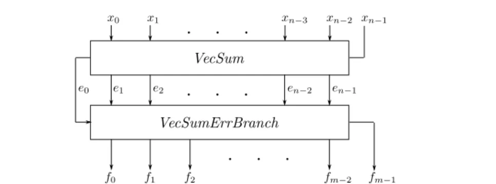
Fig. 1: Renormalization of n term-FPEs. The VecSum box performs Alg. 4 of Fig. 2, and the VecSumErrBranch box, Alg. 5 of Fig. 3.
The reduced renormalization algorithm (Algorithm 3, illustrated in Fig. 1) is made up with two different layers of chained 2Sum. It receives as input an array with terms that overlap by at most d digits, with d ≤ p − 2. Let us first define this concept.
Definition 31 Consider an array of FP numbers: x0, x1, . . . , xn−1. According
to Priest’s [17] definition, they overlap by at most d digits (0 ≤ d < p) if and only if ∀i, 0 ≤ i ≤ n − 2, ∃ki, δi such that:
2ki ≤ |x i| < 2ki+1, (1) 2ki−δi≤ |x i+1| ≤ 2ki−δi+1, (2) δi≥ p − d, (3) δi+ δi+1≥ p − zi−1, (4)
where zi−1 is the number of trailing zeros at the end of xi−1 and for i = 0,
It was proven in [10] that the algorithm returns an ulp-nonoverlapping expansion: Proposition 32 Consider an array x0, x1, . . . , xn−1of FP numbers that overlap
by at most d ≤ p − 2 digits and let m be an input parameter, with 1 ≤ m ≤ n − 1. Provided that no underflow / overflow occurs during the calculations, Algorithm 3 returns a “truncation” to m terms of an ulp-nonoverlapping FP expansion f = f0+ . . . + fn−1 such that x0+ . . . + xn−1= f .
For the sake of simplicity, the 2 levels are represented as variations of the Algorithm VecSum of Ogita, Rump, and Oishi [20, 16], and treated separately. The proof was done using intermediate properties for each layer. Also, at each step it was proved that all the 2Sum blocks can be replaced by Fast2Sum ones.
First level (line 1, Algorithm 3) The error-free transforms can be extended to work on several inputs by chaining, resulting in “distillation” algorithms [19]. The most frequently used one is VecSum (Fig. 2 and Algorithm 4). It is a chain of 2Sum that performs an error-free transformation on n FP numbers.
Algorithm 4 VecSum (x0, . . . , xn−1) [20, 16].
Input: x0, . . . , xn−1FP numbers.
Output: e0+ . . . + en−1= x0+ . . . + xn−1.
sn−1← xn−1
for i ← n − 2 to 0 do (si, ei+1) ← 2Sum(xi, si+1)
end for e0← s0
return e0, . . . , en−1
Fig. 2: VecSum with n terms. Each 2Sum [15] box outputs the sum to the left and the error downwards.
The first level consists in applying Algorithm 4 on the input array, from where we obtain the array e = (e0, e1, . . . , en−1).
In [10] the following theorem was proved:
Proposition 33 After applying the VecSum algorithm on an input array x = (x0, x1, . . . , xn−1) of FP numbers that overlap by at most d ≤ p − 2 digits, the
output array e = (e0, e1, . . . , en−1) is S-nonoverlapping and may contain
Also, it was shown that for all arrays that satisfy the input requirements 2Sum (6 FP operations) can be replaced by Fast2Sum (3 FP operations).
Second level (line 2, Algorithm 3) This level is applied on the array e obtained previously. This is also a chain of 2Sum, but now we start from the most significant component. Also, instead of propagating the sums we propagate the errors. If however, the error after a 2Sum block is zero, then we propagate the sum (this is shown in Figure 3). In what follows we will refer to this algorithm by VecSumErrBranch (see Algorithm 5).
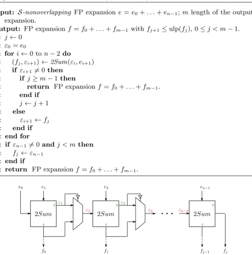
Algorithm 5 VecSumErrBranch (e0, . . . , en−1)
.
Input: S-nonoverlapping FP expansion e = e0+ . . . + en−1; m length of the output
expansion.
Output: FP expansion f = f0+ . . . + fm−1with fj+1≤ ulp(fj), 0 ≤ j < m − 1.
1: j ← 0 2: ε0= e0
3: for i ← 0 to n − 2 do 4: (fj, εi+1) ← 2Sum(εi, ei+1)
5: if εi+16= 0 then 6: if j ≥ m − 1 then 7: return FP expansion f = f0+ . . . + fm−1. 8: end if 9: j ← j + 1 10: else 11: εi+1← fj 12: end if 13: end for 14: if εn−16= 0 and j < m then 15: fj← εn−1 16: end if 17: return FP expansion f = f0+ . . . + fm−1.
Fig. 3: VecSumErrBranch with n terms. Each 2Sum box outputs the sum downwards and the error to the right. If the error is zero, the sum is propagated to the right.
For this algorithm we can also use Fast2Sum instead of 2Sum. The following property holds:
Proposition 34 Let e be an input array (e0, . . . , en−1) of S-nonoverlapping
terms and 1 ≤ m ≤ n the required number of output terms. After applying VecSumErrBranch, the output array f = (f0, . . . , fm−1), with 0 ≤ m ≤ n − 1
satisfies |fi+1| ≤ ulp(fi) for all 0 ≤ i < m − 1.
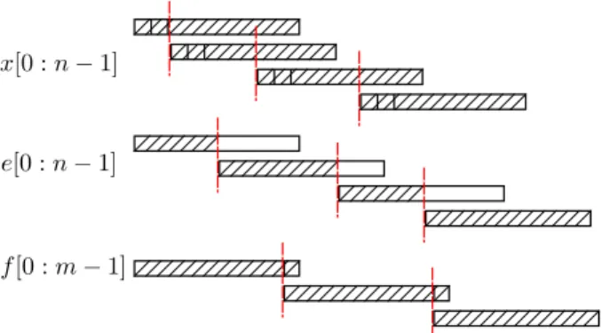
Fig. 4 gives an intuitive drawing showing the different constraints between the FP numbers before and after the two levels of Algorithm 3. The notation is the same as in Fig. 1.
Fig. 4: The effect of Algorithm 3: x is the input FPE, e is the sequence obtained after the 1st level and f is the sequence obtained after the 2nd level.
Remark 35 In the worst case, Algorithm 3 performs n − 1 Fast2Sum calls in the first level and n − 2 Fast2Sum calls plus n − 1 comparisons in the second one. This accounts for a total of 7n − 10 FP operations.
4
Formal proof
Let us now dive into what exactly is formally proved and how. We assume a FP format with radix 2 and precision p, that includes subnormals.
4.1 Prerequisites
A big difference between pen-and-paper proofs and formal proofs is the use of previous theorems. The proof in [10] relies on a result by Jeannerod and Rump [9] about an error bound on the sum of n FP numbers. In a formal proof, we need the previous result to be also formally proved (in the same proof assistant). As the Coq formal library of facts does not grow as fast as the pen-and-paper library of facts, we usually end up proving more results than expected, in particular, the result of Jeannerod and Rump does not belong to the Flocq library. Theorem 41 (error sum n, from [9]) Let l be a list of n FP numbers. Define e = Pn
i=0li and a =
Pn
i=0|li|. Let f = ⊕ n
i=0li be the computed sum. Then
The formal proof follows exactly the pen-and-paper proof from [9] without any problem. Note that the pen-and-paper result is more generic than the Coq one: it does not enforce the parenthesis, while we precisely choose where the parentheses are. As underflowing additions are correct, this holds even when subnormals are involved.
4.2 Formal proof of the first level
As explained in Section 3, Algorithm 3 has two steps. Let us deal with its first step, the VecSum algorithm (Algorithm 4).
Formalization of the VecSum algorithm A generic VecSum g algorithm is defined. Indeed, VecSum is an iteration of a 2Sum operator, where the sum is given to the next step, but we may imagine a VecSum with another operator, or with a 2Sum operator, where the error is given to the next step (this is the case of the third step of the renormalization algorithm described in [10]). Many basic lemmas apply on all these examples and it is better to factorize them.
The Coq definition is a fixed-point operator applying on a list. The variant (for the termination) is n, that will be the length of the list l.
F i x p o i n t V e c S u m _ g _ a u x ( n : nat ) ( l : l i s t R ) { s t r u c t n } : l i s t R := m a t c h n , l w i t h | 0 , nil = > nil | 1 , x :: nil = > x :: nil | S n , x :: y :: l = > ( f x y ) :: ( V e c S u m _ g _ a u x n ( x + y -( f x y ) :: l )) | _ , _ = > nil end . F i x p o i n t V e c S u m _ g ( l : l i s t R ) : l i s t R := V e c S u m _ g _ a u x ( l e n g t h l ) l .
We prove various lemmas, including the fact that the output list has the same size as the input list and that the sum of the values of the input list is the same as the sum of the values of the output list.
Another point is that each value of the output list is exactly known from the input list (in the second level, we have tests that make this statement more com-plex). Taking the notations from Figure 2, the value e0 (the last one computed)
is the FP sum of all the xis. Using our formal definition, this means that the last
element of the list is the iterated of the function fun x y =>x+y-(f x y). As for the i-th element, it is proved to be f (si+1, xi+1), where xk is the k-th element
of the list and sk is the iterated of the function fun x y =>x+y-(f x y) on the
first k elements of the list. Note that lists are “numbered” from 0 to their size minus 1.
VecSum algorithm property Now let us deal with what is to be proved for this algorithm. In this case f will be the addition error function. We first look into the requirements on the input and output expansions. Let d be a positive integer such that d ≤ p − 2, and the input an expansion with numbers that overlap by at most d digits. Formally, it is an expansion with a certain predicate IVS P (for Input of VecSum Property). This property linking two reals x and y can be stated as follows: |y| < 2dulp(x). As d ≤ p − 2, it would intuitively mean
that the expansion is clearly decreasing (as seen in Figure 4), but this is not the case when dealing with subnormal numbers. For instance, consider the smaller positive (subnormal) FP number η, then this property holds for η and himself, for η and 2η, and for 2η and η.
This is the reason why we choose:
IV S P (x, y) = 2p−dulp(x) ≤ ulp(y)
It is equivalent with the previous definition for normal numbers, but implies |x| ≤ |y|, even when subnormals appear. Another interesting property is the fact that IV S P (x, y) implies that y is normal.
The output of the expansion is supposed to be S-nonoverlapping (see Defi-nition 25). We choose the simple defiDefi-nition:
OV S P (x, y) := ∃e, n : Z, y = n · 2e∧ |x| < 2e.
Said otherwise, there exists an exponent e such that y can be expressed with exponent e and |x| < 2e. This e is an overestimation of the uls(x) of Definition 24.
Proof of the VecSum algorithm property Here is some excerpt of the proof in [10]:
|xj+1| + |xj+2| + · · · ≤
≤ [2d+ 22d−p+ 23d−2p+ 24d−3p+ . . . ] ulp(xj)
≤ 2d· 2p/(2p− 1) · ulp(xj).
This is partly wrong! In fact the geometric series should be bounded by: 2d+ 22d−p+ 23d−2p+ 24d−3p+ · · · ≤ 2d/(1 − 2d−p).
The proof can be fixed as the two inequalities were coarse enough, so there is no problem at this point.
A small gap in [10] is that it does not handle underflow. We did that in the formal proof without many problems. Given that the input list is an expansion with the IV S P property, there can be at most one subnormal FP number (at the end). This implies a special treatment for one-element lists (which is not difficult) or lists with only one non-zero element (also not difficult) and taking care of the last element in all other cases. Furthermore, [10] proves that the output is non-overlapping assuming two successive outputs are non-zeros. Unfortunately, this does not cover the most complex case: a non-zero output
followed by one (or more) zero output, due to (partial) cancellation, and then another non-zero output. When considering the outputs, if eiand ei+1 are
non-zero, the corresponding siis bigger than si+1so that the exponent of siis bigger
than that of si+1 (property used in the proof in [10]). Yet, if ei and ei+2 are
non-zero, but ei+1 = 0, then the exponents of si and si+2 may be in any order,
and the proof does not hold anymore. We therefore needed several additional lemmas.
Lemma 42 We assume we have an expansion l = (xi) with the IV S P property
with the length smaller than 2 + 2p−1. Then
– Except if the (xk)k=i to (n−1) are all zeros, then si6= 0.
– If xi× si+1≥ 0, then ulp(si+1) ≤ ulp(si).
– If xi× si+1< 0 and |xi| ≤ 2|si+1|, then ei+1= 0.
– If xi× si+1< 0 and 2|si+1| < |xi|, then ulp(si+1) ≤ ulp(si).
– If xi× si+1< 0 and |xi| ≤ 2|si+1|, then ulp(si) ≤ ulp(si+1).
– If xi× si+1< 0 and |xi| ≤ 2|si+1| and xi−16= 0, then ulp(si+2) ≤ ulp(si).
The lemma corresponds to various possibilities, including partial cancellation. The main result is then the following one:
Theorem 43 (incr exp sj) Assuming an expansion l = (xi) with the IV S P
property, such that all xk6= 0, and such that its length is smaller than 2 + 2p−1.
For all i ≤ j between 0 and the length of l, we have ulp(si) ≤ max (ulp(sj), ulp(sj+1)) .
In other words, if the exponent of sj does not have the wanted property, then
the exponent of sj+1does. From this result, we deduce the main theorem of the
VecSum algorithm:
Theorem 44 (VecSum correct) Assuming an expansion l with the IV S P prop-erty and such that its length is smaller than 2 + 2p−1, then V ecSum(l) has the
OV S P property.
To prove the OV S P property, we just have to exhibit an exponent and prove its properties. Using the previous theorem, we exhibit the maximum between the exponents of sj and sj+1, and the rest of the proof is straightforward. There are
special cases, e.g., small lists, or handling e0, which is not the same as the others
ei, or input lists with zeros. Yet, in the formal proof this is handled (with care)
more easily than the exponent problem explained above. Note that we need a maximum size of the list: here 2 + 2p−1, meaning more than 4.5 × 10¹⁵ in
binary64 and more than 8 million in binary32. As done in [10], we also prove that a Fast2Sum can be used instead of a 2Sum at every level of the algorithm. 4.3 Formal proof of the second level
Contrary to the formal proof of the first level, where we uncovered several diffi-culties, the formal proof of the second level was much simpler. Two additional features are the handling of subnormal numbers, which was trivial, and some discussions about the last two terms of the output list.
Formalization of the VecSumErrBranch algorithm As was done for Vec-Sum, we define in Coq the formal version of VecSumErrBranch. It is more com-plicated and was therefore not put here. Refer to Figure 3 for a more under-standable version. We proved several lemmas, including the fact that the sum of the values of the input list is the same as the sum of the values of the output list. We also prove that the output list has a smaller or equal size than the input list.
VecSumErrBranch algorithm property A difficulty is the need to reverse the list. VecSum was taking care of the values from the smallest to the largest, while VecSumErrBranch manipulates the values from the largest to the small-est.The input property of the expansion is the OVS P property on the reverse list, meaning an expansion with the property
fun x y ⇒ OV S P (y, x).
As for the output property, we only have the ulp-nonoverlapping property, with the definition
OV SB P (x, y) := |y| ≤ ulp(x).
Proof of the VecSumErrBranch algorithm property The input expansion has the S-nonoverlapping property, hence we can apply this lemma that will be helpful for our induction:
Lemma 45 Let us assume that (a :: b :: l) is an expansion with the OV S P (y, x) property. Then
– (a + b :: l) is an expansion with the OV S P (y, x) property. – (◦(a + b) :: l) is an expansion with the OV S P (y, x) property.
– (a + b − ◦(a + b) :: l) is an expansion with the OV S P (y, x) property. Now we need to exhibit the first value output by VecSumErrBranch. It is the sum of several of the eis, in unknown number:
Lemma 46 Let l = (ei) be an expansion with the OV S P (y, x) property. We
assume that it is non-empty and has no zeros. Define x = e0⊕Pni=1ei. There
exists an integer n and a list l0 such that:
either x 6= 0 or (x = 0 ∧ l0 is empty) and VecSumErrBranch(l) = x :: l0.
Note that the sum of (ei)1≤i≤n is exact. This is because ei is kept to be
propa-gated in the test when the error is zero, meaning the addition was exact. All there is left to prove is that the OV SB P (ulp-nonoverlapping) property is obtained with such terms:
Lemma 47 Let us assume that (b :: a :: l) is an expansion with the OV S P (y, x) property and that b + a − b ⊕ a 6= 0. Let l = (ei). Then
OV SB P b ⊕ a , ◦ (b + a − b ⊕ a) + n X i=0 ei ! ! .
Then, we can prove the main theorem of the VecSumErrBranch algorithm: Theorem 48 Assume an expansion l with the OV S P (y, x) property. Then, V ecSumErrBranch(l) has the OV SB P property.
As before, we take care of inputs with zeros using a special treatment. We also formally prove that the Fast2Sum operator can be used at every level.
A last point is that the output list is (nearly) non-zero. Due to the test, most output values cannot be zeros. All the (fi)i=0 to j−2are non-zeros, but the last
two terms fj−1 and fj may be zeros. Note that fj is zero if and only if the list
is composed only of zeros.
5
Conclusion
The renormalization algorithm is a call to the previously-defined functions, and the proofs are successive calls to the previous proofs. Here is a final Coq excerpt for the renormalization algorithm formal verification.
1 C o n t e x t { p r e c _ g t _ 0 _ : P r e c _ g t _ 0 p }. 2 V a r i a b l e d : Z . 3 H y p o t h e s i s d _ b e t w : (0 < d <= p - 2 ) % Z . 4 5 V a r i a b l e l : l i s t R . 6 H y p o t h e s i s Fl : F o r a l l f o r m a t l . 7 H y p o t h e s i s Hl : I n p u t V e c S u m d l . 8
9 Let res := V e c S u m E r r B r a n c h ( rev ( V e c S u m l )). 10 11 L e m m a R e n o r m _ 1 : F o r a l l f o r m a t res . 12 L e m m a R e n o r m _ 2 : 13 f o l d _ r i g h t R p l u s 0 l = f o l d _ r i g h t R p l u s 0 res . 14 L e m m a R e n o r m _ 3 : INR ( l e n g t h l ) <= 2 + b p o w ( p - 1) - > 15 O u t p u t V e c S u m E r r B r a n c h res .
The hypotheses are as follows: p > 0 (Line 1), 0 < d ≤ p − 2 (Lines 2–3). The input is a list of reals called l (Line 5). This list is a list of FP numbers (Line 6) and has the IV S P property (Line 7).
The result of the renormalization is then res which is the application of VecSumErrBranch on the reverse of the application of VecSum to l (Line 9).
We then have the three proved lemmas. The first one says that the result is a list of FP numbers (Line 11), the second one says that the sum of the
values resulted is equal to the sum of the values of the input l (Line 12–13), and the third one is the expected property: it is an expansion with the OV SB P property (ulp-nonoverlapping) (Line 14–16). This was fully proved in the Coq proof assistant within a few thousand lines:
spec proof file
74 497 AboutFP.v 200 1049 AboutLists.v 19 24 Renormalization.v 168 1162 VecSum1.v 93 975 VecSumErrBranch.v 554 3707 total
AboutFP includes the result of the error of FP addition from [9]. AboutLists includes results about parts of lists (such as n first elements, n last elements).
A missing part in the formal verification is the handling of overflow, as Flocq does not have an upper bound on the exponent range. It is not a real flaw, as an overflow would produce an infinity or a NaN at the end of the algorithm as only additions are involved.
This work was unexpectedly complicated: the formal verification was tedious due to many gaps, both expected (e.g., underflow) or unexpected (error in [10], handling of intermediate zeros that greatly modifies the proofs). More precisely about the intermediate zeros, let us assume that the result of the renormaliza-tion is (y0, y1, y2, 0, y3, y4, 0, y5, 0, 0, 0) with the yi6= 0. Then the pen-and-paper
theorem of [10] ensures that OV S P (y0, y1), OV S P (y1, y2), and OV S P (y3, y4).
Our theorem formally proved in Coq ensures that OV S P (y0, y1), OV S P (y1, y2),
OV S P (y2, y3), OV S P (y3, y4), and OV S P (y4, y5). Interleaving zeros may seem
a triviality as zeros could easily be removed, except that this is costly as it in-volved testing each value. For this basic block, it is much more efficient to handle zeros inside the proof than to remove them in the algorithm.
We had some hope to be able to automate that kind of proofs, as many such algorithms exist in the literature, but this experiment has shown that, even from a detailed and reasonable pen-and-paper proof, much remains to be done to get a formal one. This paper shows that complex algorithms in FP arithmetic really need formal proofs: it is otherwise impossible to be certain that special cases have not been forgotten or overlooked in the pen-and-paper proof, as was the case here.
References
1. Abad, A., Barrio, R., Dena, A.: Computing periodic orbits with arbitrary precision. Phys. Rev. E 84, 016701 (Jul 2011)
2. Bailey, D.H., Borwein, J.M.: High-precision arithmetic in mathematical physics. Mathematics 3(2), 337 (2015)
3. Boldo, S.: Iterators: where folds fail. In: Workshop on High-Consequence Control Verification. Toronto, Canada (Jul 2016)
4. Boldo, S., Daumas, M.: A mechanically validated technique for extending the avail-able precision. In: 35th Asilomar Conference on Signals, Systems, and Computers. pp. 1299–1303. Pacific Grove, California (2001)
5. Boldo, S., Melquiond, G.: Flocq: A Unified Library for Proving Floating-point Algorithms in Coq. In: Proceedings of the 20th IEEE Symposium on Computer Arithmetic. pp. 243–252. T¨ubingen, Germany (Jul 2011)
6. Fousse, L., Hanrot, G., Lef`evre, V., P´elissier, P., Zimmermann, P.: MPFR: A Multiple-Precision Binary Floating-Point Library with Correct Rounding. ACM Transactions on Mathematical Software 33(2) (2007), available at http://www. mpfr.org/
7. Hida, Y., Li, X.S., Bailey, D.H.: Algorithms for quad-double precision floating-point arithmetic. In: Burgess, N., Ciminiera, L. (eds.) Proceedings of the 15th IEEE Symposium on Computer Arithmetic (ARITH-16). pp. 155–162. Vail, CO (Jun 2001)
8. IEEE Computer Society: IEEE Standard for Floating-Point Arithmetic. IEEE Standard 754-2008 (Aug 2008)
9. Jeannerod, C.P., Rump, S.M.: Improved error bounds for inner products in floating-point arithmetic. SIAM Journal on Matrix Analysis and Applications 34(2), 338– 344 (Apr 2013)
10. Joldes, M., Marty, O., Muller, J.M., Popescu, V.: Arithmetic algorithms for ex-tended precision using floating-point expansions. IEEE Transactions on Computers PP(99), 1 (2015)
11. Joldes, M., Muller, J.M., Popescu, V., Tucker, W.: CAMPARY: Cuda Multiple Precision Arithmetic Library and Applications, pp. 232–240. Springer International Publishing, Cham (2016)
12. Joldes, M., Popescu, V., Tucker, W.: Searching for Sinks for the H´enon Map Using a Multipleprecision GPU Arithmetic Library. SIGARCH Comput. Archit. News 42(4), 63–68 (Dec 2014)
13. Kornerup, P., Lef`evre, V., Louvet, N., Muller, J.M.: On the computation of correctly-rounded sums. In: Proceedings of the 19th IEEE Symposium on Com-puter Arithmetic (ARITH-19). Portland, OR (June 2009)
14. Laskar, J., Gastineau, M.: Existence of collisional trajectories of Mercury, Mars and Venus with the Earth. Nature 459(7248), 817–819 (Jun 2009)
15. Muller, J.M., Brisebarre, N., de Dinechin, F., Jeannerod, C.P., Lef`evre, V., Melquiond, G., Revol, N., Stehl´e, D., Torres, S.: Handbook of Floating-Point Arith-metic. Birkh¨auser Boston (2010)
16. Ogita, T., Rump, S.M., Oishi, S.: Accurate sum and dot product. SIAM Journal on Scientific Computing 26(6), 1955–1988 (2005)
17. Priest, D.M.: Algorithms for arbitrary precision floating point arithmetic. In: Ko-rnerup, P., Matula, D.W. (eds.) Proceedings of the 10th IEEE Symposium on Computer Arithmetic. pp. 132–144. IEEE Computer Society Press, Los Alamitos, CA (Jun 1991)
18. Priest, D.M.: On Properties of Floating-Point Arithmetics: Numerical Stability and the Cost of Accurate Computations. Ph.D. thesis, University of California at Berkeley (1992)
19. Rump, S.M., Ogita, T., Oishi, S.: Accurate floating-point summation part I: Faith-ful rounding. SIAM Journal on Scientific Computing 31(1), 189–224 (2008) 20. Shewchuk, J.R.: Adaptive precision floating-point arithmetic and fast robust
![Fig. 2: VecSum with n terms. Each 2Sum [15] box outputs the sum to the left and the error downwards.](https://thumb-eu.123doks.com/thumbv2/123doknet/14507295.529024/8.918.200.726.490.803/fig-vecsum-terms-sum-outputs-left-error-downwards.webp)