The cost of noise reduction in helicopters

U

THE COST OF

NOISE REDUCTION

IN HELICOPTERS

HENRY FAULKNER

November 1971

FTL Report R71-5

MASSACHUSETTS INSTITUTE OF TECHNOLOGY Flight Transportation Laboratory

THE COST OF NOISE REDUCTION IN HELICOPTERS

by

Henry Faulkner

Report FTL R71-5 November 1971

ACKNOWLEDGEMENTS

The original helicopter design computer program used for these studies was written by Michael Scully as work performed under ARO Contract DAHCO4. He and Professor Robert Simpson also offered many helpful suggestions and comments.

This work was performed under Contract DOT-TSC-93, DSR No. 72915, from the Transportation Systems Center, Department of Transportation, Cambridge, Massachusetts.

ABSTRACT

The relationship between noise reduction and direct operating cost was studied for transport helicopters. A

large number of helicopter preliminary designs was generated with the help of a computer program. Vehicles were selected

to meet certain noise goals with minimum direct operating cast. this was repeated for several payloads and technology time frames. The effect of changes in the assumed mission profile was studied.

Table of Contents

Page

1.0 Introduction 1

2.0 Helicopter Design Procedures

2.1 General 4

2.2 Description of the Helicopter Design

Computer Program 4 2.3 Noise Reduction 10 2.4 Design Constants 12 3.0 Results 15 3.1 Nomenclature 15 3.2 Basic Variation 16 3.3 Size Variation 30

3.4 Time Frame Variation 37

3.5 Path Variation 42

4.0 Conclusions 51

5.0 References 52

6.0 Appendix: Definition of Helicopter

1.0 Introduction

The helicopter has become an important means of transportation in densely populated regions. Land is scarce and surface trans-portation is slow in these regions. Here the higher operating

costs of the helicopter can be offset with its small land

requirements and the resulting ability to locate numerous terminals. In the next decade helicopter transportation is expected to expand rapidly if noise abatement constraints are met.

In this report the emphasis is on helicopters for intercity transportation, covering stage lengths of 50 to 400 miles. However, the results could be applied to intraurban helicopters operating on shorter stage lengths.

In recent years a strong adverse public reaction to aircraft noise has developed. Noise reduction is now an important, if not dominant, objective in air transportation planning. The helicopter is inherently one of the quietest types of transport aircraft.

However, it is likely to operate closer to a greater number of

listeners than other types because of the small size of the terminals it operates from and the greater number of them. Therefore it is essential to the success of helicopter transportation that its

potential for low noise operations be exploited as far as possible. There are two methods of reducing the noise exposure due to aircraft operations. One is to change the flight profile. The aircraft trajectory can be moved further from the listeners, the amount of noise generated can be reduced by changing thrust, or the speed can be increased in order to reduce noise exposure time. This method of noise reduction is explored in references 8 and 9. The second method is to change the design of the aircraft to reduce the noise generated at a given distance, thrust level, and speed. The

second method is given primary emphasis here. However, substantial changes in the flight profile, which affect the design, are also considered.

It is worth remembering that existing helicopters were not designed with noise reduction as a design objective at the outset. Modifications have been made to a few existing helicopters to reduce noise, often accompanied by a significant loss of payload. This does not indicate, however, that new helicopters cannot be designed to achieve substantial noise reduction with a moderate increase

in direct operating cost. It is also worth remembering that all existing large helicopters were designed for military use, and hence a decrease in direct operating cost might be achieved by designing primarily for a civilian transport role.

The purpose of this work is to identify those design changes which can reduce noise with the minimum cost penalty and to develop the

relationship between the amount of noise reduction and the resulting cost penalty.

Miller (Reference 10) performed an initial study of these questions. By developing a series of helicopter preliminary designs, he explored the relationship between design parameters, direct operating cost, and noise generated. A computer program was used to aid in the

design iterations. Curves of hover noise versus hover tip Mach number and direct operating cost (DOC) versus hover noise were developed for a series of 80 passenger helicopters. These curves were generated by varying either the hover tip Mach number, or the thrust coefficient to solidity ratio, while holding other parameters constant.

In this work a different approach is taken using a more

noise objectives were set along with size, technology time frame (year of first flight), and operational constraints. Then all other parameters were varied to produce a vehicle with minimum direct operating cost which met the noise objectives. This was then repeated for three other levels of noise objectives to find

the relationship between noise level and direct operating cost. This basic variation was then extended to different sizes and

time frames. Finally, the effect of different operational constraints on noise and direct operating cost was examined.

2.0 Helicopter Design Procedure

2.1 General

The process for preliminary design of air vehicles can be computerized such that parametric variations can be obtained rapidly. These computer programs are now a design tool used to find the optimal configuration for a given vehicle performance requirement in terms of size, speed, range, direct operating cost, etc. Estimated noise generation is now included as one of the

performance measures of the vehicle. Other design objectives can be met at varying levels of noise, or an optimal design can be found for a specified noise level.

2.2 Description of the Helicopter Design Computer Program a) The Design Logic

The helicopter computer design program is fully described in Flight Transportation Laboratory Technical Memo 71-3 (Reference 1). This program considers only conventional pure helicopters.

(See Appendix for helicopter terminology.)

The program begins by reading input data such as cabin size, range, speed, etc. and generating constants, including atmospheric data, for later use. Calculations regarding hover performance are done for a hot day; all other calculations assume a standard day.

Then the program goes into a design procedure which is an iteration on gross weight. Initially a gross weight is estimated based on the design payload; on succeeding iterations the previous

gross weight is used. The rotor -is then designed considering both cruise and hover. It is assumed that there are two rotor angular velocities: the rotor turns at hover rpm when the advance ratio

is less than 0.325 and cruise rpm otherwise. Next the fuselage is sized and parasite drag is calculated. Then the power plant and drive system is sized to the maximum of cruise and hover requirements. If hover rpm is less than cruise rpm then the

installed power required for hover is increased to account for

reduced engine output below rated rpm. This completes the selection of design parameters.

The vehicle is then flown through the design mission to find

the fuel consumed. Nine phases in the mission profile are considered: hover, vertical climb, acceleration to climb advance ratio,

unaccelerated climb to cruise altitude, acceleration to cruise, cruise, undecelerated descent, deceleration to hover, and vertical descent. The time, distance and fuel consumed in each phase is

calculated. An input table of rotor lift-to-drag ratio as a function of advance ratio and thrust coefficient to solidity ratio is used to estimate performance above advance ratio .325.

Then the component weights are calculated, resulting in a new gross weight. If the difference between new and old gross weights

is greater than 10 pounds, the design procedure goes through another cycle. When the iteration is complete the parameters describing the final design are printed.

b) Vehicle operating Cost

The vehicle then is flown through various stage lengths that are less than the design range, with appropriate cruise altitudes and speeds. The time, distance, and fuel consumed for each phase of each stage is calculated, printed, and stored for use in the calculation of direct operating cost (DOC).

Then the program calculates DOC's for each stage length, breaks them down by categories, and prints this out. The DOC is calculated according to the Lockheed VTOL formula. (References 3 and 4).

c) Vehicle Noise Generation

As the last step, the program calculates the noise generated by the vehicle. There are three principal noise sources in a

helicopter: the rotors, the engine, and the transmission. Modern :ommercial helicopters are powered by turboshaft engines. The methods used to quiet these engines and the transmission are quite

straightforward and have a relatively small effect on DOC. This effect is accounted for by assuming a weight penalty in the engine.

Above 90 dB perceived noise level at 500 feet no pena-lty is assumed. The input horsepower/weight ratio is decreased approximately 20% for each 10 dB reduction below 90 dB. The weight penalty for quieting the tail rotor on single rotor ships is assumed to be insignificant. Thus noise sources other than the main rotor(s) are assumed to be quieted singificantly below the main rotor(s).

Overall sound pressure level for the rotor(s) at 300 feet

distance is calculated using the following well established formula taken from reference 5 for vortex noise. This formula is applied to all flight conditions. In cruise, the advancing blade tip

speed is used. _{-10 2 2}

L

10

log

tip

p 1

whereL = overall sound pressure, db

p

T = thrust, lb.

V =tip rotor tip speed, ft/sec /> = air density, slugs/ft3

A = total rotor blade area, ft2 B

Rotational noise was hand-calculated for a sample case using both the method of Ollerhead and Lowson (Reference 6) and a method developed in the Flight Transportation Laboratory

(Reference 7). Both results indicated that rotational noise was not significant for helicopters with low tip speeds, and thus it has not been included in the program. Recent research (Reference 12) has indicated that a large part of what used to be thought of as vortex (broadband) noise may in fact be largely composed of

rotational noise. This does not affect the accuracy of empirical predictions of overall sound pressure level, however.

Simple inverse square law attenuation is used to for observer distance other than 300 feet from the vehicle. No directivity in azimuth is assumed. The method given in Reference 6 for vortex noise is used for directivity in elevation. A factor DF is added to

the overall sound pressure level: 2

cos2 + 0.1

DF = 10 log Co $+0.

10

Cos

₇₀

_0.1

where

f

a line joining the rotor hub and the observer.

This factor varies from +7.0 along the shaft axis to -.34 in the rotor plane. The overall sound pressure level is converted to perceived noise level using an assumed frequency distribution from Reference 11.

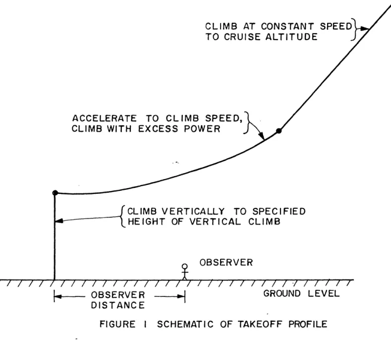
The standard takeoff profile assumed in the helicopter design program is shown in Figure 1. Climb power (1.2 times normal rated power) is used throughout the takeoff profile. During the

acceleration phase, the vehicle tries to accelerate horizontally at a given maximum acceleration, and if it has more than enough power to do this, it uses the excess power to climb. Hence the

CLIMB AT CONSTANT SPEE TO CRUISE ALTITUDE

ACCELERATE TO CLIMB SPEED,

CLIMB WITH EXCESS POWER

CLIMB VERTICALLY TO SPECIFIED HEIGHT OF VERTICAL CLIMB

OBSERVER

FIGURE I SCHEMATIC OF TAKEOFF PROFILE

OBSERVER GROUND LEVEL

profile varies depending on how much power is available and the maximum acceleration allowed. During the climb phase the vehicle

climbs at a constant forward speed. The observers are always in the plane of the takeoff profile. Varying the height of vertical

climb has the effect of shifting the flight profile up or down. Reducing the maximum acceleration causes greater excess power to be available for climb and hence has the effect of tilting the path upward during acceleration.

As the vehicle accelerates from rest to its vertical rate of climb, thrust is greater than weight and hence more noise is

generated. The noise resulting from maximum thrust is calculated and assumed to represent the noise in the first few seconds of the takeoff profile. This is called noise at liftoff.

The noise is calculated for a single observer at 15 points during the takeoff profile and output along with the time, altitude and horizongtal distance corresponding to each point. This can be repeated for observers at different distances from the takeoff point. Noise on the ground due to the vehicle passing directly overhead at cruise-altitude (peak flyover noise) is also calculated.

Noise is not calculated for the landing profile. However, the landing profile is nearly the reverse of the takeoff profile. Idle power is used for descent and deceleration. Most of the descent is made at cruise speed. Then the vehicle decelerates at a specified

allowable deceleration using excess drag for the rest of the descent to a specified height of vertical descent. Vertical descent to touchdown

is made at a specified maximum vertical descent rate to avoid entering the vortex ring state. Thus the landing profile does not differ

fundamentally from the reverse of the takeoff profile, but somewhat different distances and speeds may be involved in each phase.

2.3 Noise Reduction

This section describes the procedures involved in varying design parameters to achieve low levels of rotor noise for a given mission. (See Appendix for helicopter terminology).

The formula for overall sound pressure level for vortex noise from section 2.2 may be rewritten as follows:

10 log 3.04 x 10 (C ) . A - (V . )

[3.410 L B tip j

where C = average blade lift coefficient::=6 (CT/-) L

of the three variables, it is clear that since V . is raised tip

to the sixth power, it is dominant in reducing the overall noise level.

Consider cruise noise reduction first. Since the tip speed in the formula above is taken to be the advancing blade tip speed, cruise noise is reduced by reducing the advancing blade tip Mach number, Mat'

Now consider hover (or low speed flight) noise reduction. The rotor thrust in hover, which must remain constant, is given by the following relation:

T = A V 2 _{(C /<r)}

Th aB th T h

where / = air density for hover conditions V = rotor tip speed in hover

(C /-) = thrust coefficient to solidity ratio in hover A small decrease in hover tip speed from normal practice can be obtained by increasing (C T/c-)h to a maximum of 0.10. Beyond this value blade stall becomes critical and blade area must be increased either by increasing solidity, a-, or decreasing disc loading, DL.

I-However, changes in cruise parameters must accompany the increase in blade area because cruise thrust, T cr, must also

remain approximately constant. The following relations apply: 2 T = fcr A V (C /0-) cr B tcr T cr a M and V = cr at tcr 1 1 +1AA

where = air density for cruise conditions V = rotor rotational tip speed in cruise

tcr

(C (/-)cr thrust coefficient to solidity ratio in cruise

a = speed of sound for cruise conditions cr

= advance ratio

Thus an increase in blade area would be accompanied by a decrease in (CT

/

an increase in advance ratio or a decrease in advancing tip Mach number. Conversely, a decrease in Mat for cruise noise reduction must be accompanied by an increase in k, and increase in AB, or an

increase in (C /<-) . To reduce noise for hover and cruise conditions T cr

simultaneously, AB and would be increased and both (C /cl-)cr and Mat

would be reduced.

The noise prediction formula used here was developed from a correlation of design parameters with measurements of noise from helicopters and rotors (Reference 2). These helicopters and

rotors had solidities and disc loadings typical of designs which are unconstrained by noise considerations. As the solidity is increased and disc loading reduced to reduce noise, this empirical noise

prediction formula becomes less valid. Further experimental data on the noise generation of low disc loading high solidity rotors is

required to develop a more generalized formula. Until this is available, prediction of large noise reductions based on this formula must be regarded as preliminary. The same argument

can be applied to the method of predicting high speed rotor performance. Experimental performance data is also needed for high solidity, low disc loading rotors.

Variations in detail rotor blade geometry are not considered here. New tip planforms and twist distributions can reduce noise

somewhat beyond the levels shown here. These changes do not generally result in a significant weight or performance penalty,

and hence do not affect DOC. Therefore they do not change the nature of what is said here.

2.4 Design Constants

All of the helicopters in this report, except E70-50, are designed to be able to hover on a hot day with one engine

out.

A number of inputs to the helicopter design computer program were kept constant throughout the work reported here. The values of these are presented in Table 1.

Table 1 : Input Constants

Climb Advance Ratio

Rotor Equivalent Lift/Drag Standard Temp.

Hot Day Temp. Reserve

Rate of Vertical Descent Allowable Deceleration Utilization Depreciation Period Airframe Cost Engine Cost Insurance Rate Labor Rate - 0.30 = See Table 2. = 590 F = 950 F

= 20 min. at cruise power = 600 feet/minute = .20 g = 2300 hour/year = 12 years = 70 $/pound = 50 $/hp. = 2%/year = 5 $/hour

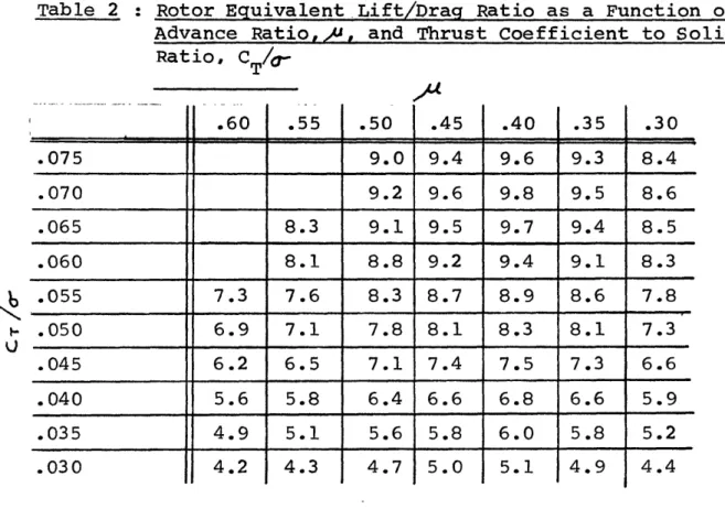
Table 2 : Rotor Equivalent Lift/Drag Ratio as a Function of Advance Ratio,uA, and Thrust Coefficient to Solidity Ratio, C /g-.60 .55 .50 A4 .45 .40

1 .35

Note : This table was derived using the performance of existing helicopters and preliminary rotor performance prediction

studies in the Flight.Transportation Laboratory. bU

U

3.0 Results 3.1 Nomenclature

The helicopter designs described here are designated by codes consisting of a letter and two numbers. The letter indicates the noisiness class according to the following mnemonics:

C - Cheap - unconstrained M - Medium - moderately quiet

Q - Quiet - very quiet

S - Silent - extremely quiet

The first number indicates the technology time frame. Here the time frame is the year in which a production prototype could be

flying, using the latest technology both in design and manufacturing. The second number indicates the size as measured by passenger

seats. For example, Q75-50 is a very quiet helicopter, designed using 1975 technology and carrying 50 passengers. An exception

to this is E70-50, which represents an approximation of a helicopter existing in 1970, the Vertol 347.

Other nomenclature is shown below:

(LPN

)to

(LPN) cr perceived noise level in cruise overhead

GW = gross weight

Vcr = cruise speed

NRP = normal rated power

(L/)r = overall lift to drag ratio in cruise

GBH = gear box factor in hover (factor used to determine the drive system limited power at hover rpm)

D = Rotor diameter

C = Rotor blade chord

H = height of vertical climb and descent vc

(a/g)max = maximum allowable forward acceleration

H =cruise altitude

cr

3.2 Basic Variation

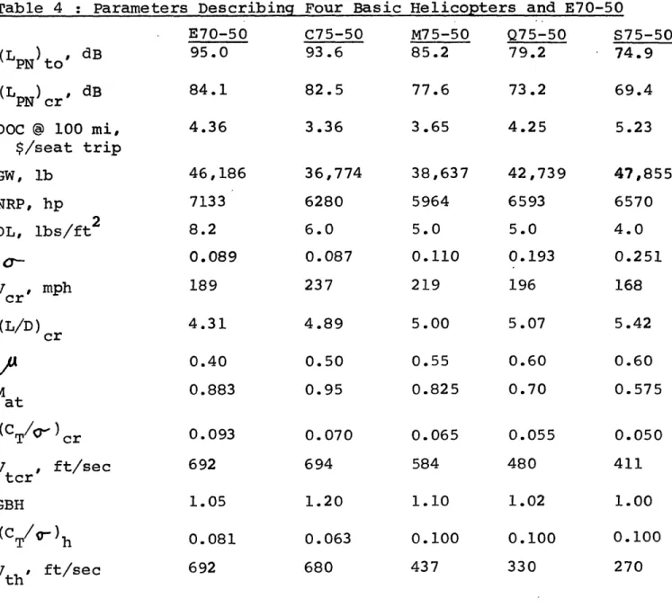
The basic variation consists of four tandem helicopters, designed to meet four different noise level objectives. The payload, design time frame, and operational constraints were kept constant as shown in Table 3. All other parameters were varied to produce vehicles which met the noise objectives with minimum direct operating cost, as shown in Table 4.

The fifth vehicle shown in Table 4, called E70-50, is an approximation to a helicopter existing in 1970, the Vertol 347. This vehicle was included to add perspective by showing what is available now. It has the same payload, range and operating constraints as the other machines, but lacks engine-out hover capability.

The C and S vehicles were chosen to represent the extremes of the noise level spectrum for this kind of aircraft. It is unlikely that any future civilian transport helicopter would be designed without regard for noise reduction, as the C vehicle is. The S vehicle, on the other hand, carries the noise reduction techniques described above to the fringe of practicality.

one of the features of the Svehicle which is most likely to be impractical is the high solidity. The rotors for the four

basic helicopters are shown to scale in Figure 2. A solidity of 0.25 has generally been considered the maximum practical in previous work in the Flight Transportation Laboratory. However, it can be argued that the practical limit is somewhat less. The sensitivity

of DOC to solidity was studied to determine how serious this problem was for the Q and S vehicles. The result, shown in Figure 3, is

Table 3 : Parameters Held Constant for Basic Variation

Seats

Time Frame Design Range

Height of Vertical Climb Cruise Altitude Maximum Acceleration = 50 = 1975 = 400 miles = 500 feet = 5000 feet = 0.25

Fig. 2 Rotors for basic helicopters.

Table 4 : Parameters Describing Four Basic Helicopters and E70-50 (LPN to' dB (LPN cr dB DOC @ 100 mi, $/seat trip GW, lb NRP, hp DL, lbs/ft2 V cr, mph (L/D) _cr

"A

5.5 S 75-50 NOMINAL 5.0 a =0.25 CUTOFF 4.5 Q 75-50 'NOMINAL 4.0 0 ₄ 0 0.100 0.150 0.200 0.250 SOLIDITY, a

that the solidity can be reduced to about 0.15 before DOC begins to rise significantly.

In general, the parameters in Table 4 show a monotonic variation with noise level. It is interesting to note that

overall lift to drag ratio increases with decreasing noise level ecause cruise speed is decreasing. The variation of NRP seems slightly erratic. It decreased from c75 - 50 to M75 - 50 because cruise power required is decreasing. In Q75 - 50, however, NRP is set by hover power requirements which have increased from

M75 - 50 to Q75 - 50. The hover power requirements would increase

still further in S75 - 50 except that disc loading was decreased.

It should be borne in mind that cruise noise (peak flyover noise) and liftoff noise are being reduced simultaneously here. A particular proportion of cruise noise reduction to liftoff noise reduction has been assumed, about 3 dB in cruise for each 5 dB at liftoff. The

interrelationships between cruise and low speed parameters were discussed in section 2.3. Different proportions between the noise reduction goals would produce different optimum vehicles.

DOC is plotted against liftoff noise and cruise noise in Figures 4 and 5 respectively. These are the basic cost vs. noise reduction relationships that were sought. As expected, noise reduction returns, per unit increase in DOC, diminish as we move

toward quieter vehicles.

DOC at 100 miles stage length was taken as representative of typical intercity operations. DOC at other stage lengths can be

found in Figure 6.

Liftoff noise was chosen here as a measure of terminal area noise because it is independent of the takeoff path. However, it is clearly only one dimension of the terminal noise picture.

5.5

Q

S 75-50

50 SEATS

5.0

1975 TECHNOLOGY (EXCEPT E70)

1-4.5

<

LU

Q 75-50E7-0>

-0C

_75-50

L PN

dB

50 SEATS

1975 TECHNOLOGY (EXCEPT E70)

E70-50

Q

75-50

M75-50

C 75-50

LPN, dB

Fig. 5 DOC @ 100 mi. vs cruise noise @ 5000 ft altitude for basic helicopters.

S 75-50

1-

I- 10 C 75-50 5 -0 0 100 200 300 400 STAGE LENGTH, mi

Therefore noise vs. time histories were found for three of the helicopters, as heard by observers at three distances from the

liftoff point. These are shown in Figures 7, 8 and 9. The directivity function gives maximum noise along the rotor shaft

axis, and minimum noise in the rotor plane. Thus the maximum noise occurs when the aircraft is overhead in all cases. The first dip in the noise vs. time curves is due to the decrease in thrust as the vehicle moves from vertical acceleration into

steady state vertical climb. Noise increases again at the top of vertical climb because the rotor plane has moved further from the observer and thus the directivity function is stronger. Noise decreases again as the rotor plane is tilted toward the observer at the start of horizontal acceleration. Then, as the vehicle

moves toward the overhead position, noise builds rapidly toward the peak.

To clarify the space-time relationships, the takeoff profiles for C75-50 and Q75-50 are plotted in Figure 10. Notice that C75-50 moves through its profile much more rapidly, but the acceleration phase (curved portion of the profile) takes up much more space. Q75 - 50 is 9 - 13 dB quieter than C75 - 50 at corresponding

points in space, but Q75 - 50 reaches these points later in time. This is due to the lower gear box limited power for 075 - 50.

The curves show that, for any given vehicle, the peak noise heard by each of the three observers is about the same. This is an indication that a greater height of vertical climb should be

considered. This will be discussed further in section 3.5.

100 95 90 ao 85 80 0 20 40 60 80 100 120

TIME, SEC

Fig. 7 Noise vs time from liftoff for 3 helicopters with observer at 500 ft.

100 95 901- 851-W~ -J

E70-50

,

I

CI75-50

*At

_I

1-Q 75-50

75

TIME, SEC

100 95 90 80 g

Q

75-50x

\

TIME, SEC

Fig. 9 Noise vs time from liftoff for 3 helicopters with observer at 1500 ft.

28

NUM3ERED POINTS INDICATE TIME FROM LIFTOFF IN SECONDS

Q

75-50

HOR IZONTAL DI STANCE FROM LIFTOFF, ft.

Fig. 10 Altitude vs distance from liftoff for 2 helicopters.

Q0 < --500 F-43. 23.3 - -4-46.5 14.6 i 24.8 010 2000I

3.3 Size variation

In the basic variation the payload was kept fixed at 50 seats. This was then extended by developing equivalent variations for

20, 80, and 110 seats.

Except for seats, the parameters in Table 3 were kept the same. Table 5 contains a portion of Table 4 which was used again for the variation of noise for a given size. Note that noise levels are not shown since a larger vehicle will be noisier, other parameters being kept constant. Keeping these parameters constant assumes that the optimal values for 50 seats are optimal for the other sizes as well.

The parameters shown in Table 6 were changed along with size. Fuselage planform outlines are shown in Figure 11. A large pro-portion of the planform area is devoted to the cabin. This is possible because these aircraft are assumed to be unpressurized and the short design range should allow lavatory and galley space to be small.

It was not within the scope of this work to make a detailed study of the range of sizes over which either the single main rotor or tandem configuration is optimal. However, it was felt that

the single rotor configuration was superior for the 20 seat size and the tandem superior for the 80 and 110 seat sizes. Both

configurations were considered for the 50 seat size. Within the accuracy of the design procedures used here, the tandem was very

slightly, but not significantly, superior.

DOC vs. liftoff noise and DOC vs. cruise noise are plotted in Figures 12 and 13, respectively, for the various vehicle sizes. As expected, the curves have the same shape as the basic variation,

Table 5 : Parameters for Size and Time Frame Variations DL, lb/ft2 gcr , mph M at T cr Vtcr, ft/sec GBH

(C

/0-)h

Table 6 : Parameters Varied with Size Seats 20 50 80 110 Flight Crew 2 2 2 3 Stewardesses 1 2 2 3 Fuselage Length, ft. 37.6 59.8 73.0 86.2 Fuselage Diameter, ft. 7.8 9.4 11.0 12.6 Seats Abreast 3 4 5 6 Doors 1 2 3 4 Payload Weight, lb. 4200 10,400 16,400 22,600 Furnishings Weight 1800 3650 5240 6880

Avionics and Instruments wt. 700 840 900 1000

Main Rotors 1 2 2 2

Number of Engines 2 3 3 3

I1~L t I I I I I I I I I I ILA

I

1

Fig. 11 Fuselage planform layouts. 110 SEATS

50 SEATS

c

L.V J LrAI 3 I-6 5 4

50 SEATS

3

80 SEATS

2

LPN, dB

1975 TECHNOLOGY

20 SEATS

50 SEATS

SEATS

110 SEATS

LPN, dB

Fig. 13 DOC @ 100 mi. vs cruise noise

@

35

a:

C)

4

20 -fl-

_{20 SEATS,}

50 SEATS\

110 SEATS

5

-

80 SEATS

STAGE LENGTH, mi.

with the curves for larger vehicles being lower. However, a very significant result is indicated by the crossing of the 80 seat curve and the 110 seat curve in both figures. It is a generally accepted rule in transport aircraft economics that a larger vehicle will have a lower direct operating cost per seat. These curves show that, if certain noise objectives are to be met, this is no longer true; there is an optimum aircraft size based on DOC alone.

Again DOC at 100 miles stage length was chosen as representative. The DOC is plotted vs. stage length in Figure 14 for the Q series

vehicles. These vehicles are represented by the second point from the left on each of the DOC vs. noise curves. DOC vs. stage

length curves for C, M, and S series vehicles are very similar. The terminal noise vs. time history, for a given vehicle

series, moves upward slightly for larger size, but does not change shape.

3.4 Time Frame Variation

Holding the size fixed' at 50 seats, the basic variation was

extended along another dimension, the technology timeframe..Variations equivalent to the basic variation, of 1975 time frame, were

developed for time frames of 1970, 1980 and 1985. As mentioned earlier, the time frame is the year in which a production prototype could be flying, using the latest technology both in design and manufacturing.

The parameters in Table 3, except time frame, were kept the same as the basic variation. The parameters.of Table 5 were used

again for the variation of noise for a given time frame. As with the size variation, it is assumed that these parameters remain optimal, in this case for different time frames.

The parameters that are varied with time frame are shown in Iinmmi.imii.i IUEEIIIEMIIIIIUIEEEIM Mliii

Table 7 : Parameters Varied With Time Frame

Time Frame

E70-50 1970 1975 1980 1985 Fuselage Drag Factor 3.4 3.0 2.5 2.0 1.8 Hub and Pylon Drag Factor 0.0310 0.0250 0.0225 0.0200 0.0190

Engine Power/Weight 5.0 - - -

-C series - 5.0 7.0 9.0 10.0

M series - 4.5 6.5 8.5 9.5

Q series - 4.0 6.0 8.0 9.0

S series - 3.5 5.5 7.5 8.5

Specific Fuel Consumption 0.52 0.52 0.43 0.40 0.37 Rotor Weight Factor 1.20 1.05 0.90 0.80 0.70 Drive System Weight Factor 0.82 0.80 0.70 0.60 0.50 Fuselage Weight Factor 1.10 1.00 0.95 0.90 0.85

Note : The drag and weight factors multiply the appropriate formulae.

50

SEATS

61-1970

E70-50

F-1980

LPN dB

Fig. 15 DOC @ 100 mi. vs liftoff noise @ 500 ft for varying time frame.

0-C-)

-50 SEATS

E70-50

1985

LPN, dB

Fig. 16 DOC @ 100 mi. vs cruise noise @ 5000 ft altitude for varying time frame.

(-)

15 1970 1975 1980 0- 10 1985 5 0 0 100 200 300 400 STAGE LENGTH, mi

Table 7. The drag and weight factors used in E70 - 50, to simulate the Vertol 347, are somewhat higher than for 1970 time frame.

While the 347 prototype did make its first flight in 1970, it does not represent the degree of advance that could have been

achieved by a complete design and development effort. The parameters in Table 7 were derived by using engineering judgement and knowledge of specific projected technological developments to extrapolate

historical trends.

DOC vs. liftoff noise and DOC vs. cruise noise are plotted in Figures 15 and 16 respectively. E70 - 50 is shown for added perspective. Again the curves have the same shape as the basic variation with the curves for later vehicles falling lower. It

is interesting to note that the quietest 1985 vehicle costs very little more than the noisiest 1970 -vehicle. In other words, the technology

improvements can offset the penalties of a moderate pace of noise reduction.

Again DOC at 100 miles stage length was chosen as representative. The DOC is plotted vs. stage length in Figure 17 for the Q series

vehicles. These vehicles are represented by the second point from the left on each of the DOC vs. noise curves. DOC vs. stage length curves for C, M, and S series vehicles are very similar.

The terminal noise vs. time history, for a given vehicle series, moves downward slightly for later time frames, but does not change shape.

3.5 Path Variation

This section considers variations on the design mission

assumed for all the previous variations (See Table 3). It should be remembered that here each change in a path parameter represents

a new vehicle designed for that mission, not the same vehicle flying a different path. The path variations here are based on

the 075 - 50 vehicle and the parameters under Q in Table 5 are used.

Thus Q75 - 50 designates a family of different vehicles in this

section.

Consider terminal path variations first. We can vary height of vertical climb and descent, which here are always equal. Noise vs. time histories for various heights of vertical climb are plotted

in Figure 18. For a 1500 foot climb, the peak noise is still definitely overhead, but it is significantly reduced. The longer period of lower intensity noise prior to the peak may contribute to annoyance, however. DOC-is plotted vs. stage length for the same vertical climb variation in Figure 19. The higher vertical climbs

cost very little for stage lengths of greater than 50 miles. The maximum allowable acceleration is another terminal path parameter which may be changed. As discussed in section 2.2 (c), reducing the maximum acceleration has the effect of tilting the

flight path upward in the acceleration phase. This can be seen in Figure 20 where takeoff profiles are plotted for two extremes of allowble acceleration. Noise vs. time histories for these two values and an intermediate one are shown in Figure 21. Reducing allowable acceleration reduces the peak noise and causes the peak to occur slightly later. The change in DOC over this range of allowable accelerations is negligible.

Another terminal path parameter is the hover gearbox factor, GBH, which determines drive system limited power at hover rpm

(low speeds). Increasing GBH has the effect of speeding up the takeoff procedure. The noise vs. time history is shifted to the

Hv

=

250 FT

vc

I

(alg)max

=

0.25

H

500 FT

(STANDARD)

vc

H

1000 FT

vc

I\

OBSERVER AT 1000 ft

H

1500 FT

/

I

TIME,

SEC

Fig. 18 Noise vs time from liftoff for Q75-50 helicopter and varying _vc'

85

1--o

-J

|-10

N

1500 -(alg)

_max

HORIZONTAL DISTANCE FROM LIFTOFF, ft.

Altitude vs horizontal distance from liftoff for Q75-50 helicopter and two values of (a/g)max' Fig. 20

(alg) =

0.25(

80

F-

751-.,.*

701-0.15

ma

651-

VC

100

120

Fig. 21 Noise vs time from liftoff for Q75-50 helicopter and varying

(a/g)max-0

DOC increases very slightly with increasing GBH. Note that the optimum GBH is somewhat higher for noisier vehicles (See Table 4).

It can be seen that the terminal noise vs. time history can be shifted around to a considerable extent. The problem of optimizing the terminal path cannot be pursued further at present because of the lack of a generally applicable method of condensing the noise vs& time history into a single measure of annoyance.

Now consider cruise path variations. A variation of design range was not considered necessary since it would yield results similar to a small size variation. This leaves cruise altitude, and peak flyover noise (cruise noise) is plotted vs. cruise altitude

in Figure 22. DOC vs. stage length for various cruise altitudes is shown in Figure 23. Cruising higher than 5000 feet reduces flyover noise appreciably while increasing DOC only slightly.

However, structural penalties for pressurization have not been taken into account here. Hence the DOC for higher cruise altitudes is optimistic.

It is well known (References 6 and 7) that the noise directivity pattern sweeps forward as spded increases, so that the maximum

noise occurs in front of the helicopter rather than below. However, there is not sufficient data upon which to base a reliable empirical formula. Further study of helicopter cruise noise cannot be

accomplished until new experimental data are obtained.

zO S70-- -%J-J 65 60 0 0 5000 10,000 15,000 ALTITUDE, ft.

15 _-UK-t -00 HCR= 10,000 a-0 C-) H000 5 0 0 100 200 300 400 STAGE LENGTH, mi

4.0 Conclusions

I The central conclusion of this work is that good economic performance can be expected from future helicopters which have low noise generation. -By using high solidity rotors at lower disc loading, perceived noise levels at 500 feet for a 1975, 50 passenger, 400 miles design range vehicle can be kept below 85 dB. These levels are expected to be compatible with future operations from selected city center sites.

Experimental data on the noise generation and aerodynamic performance of low disc loading, high solidity rotors is urgently needed to 'improve the accuracy of the noise and performance

prediction techniques used here.

Larger helicopters have a more severe economic penalty for low noise generation. Therefore the optimum economic size in a given operation will be smaller for a quiet vehicle than for a vehicle without noise constraints.

The expected improvements in helicopter technology over the next fifteen years- can offset the economic penalties due to noise reduction. Thus the direct operating cost of a very quiet 1985 vehicle can equal that of a present day vehicle designed without regard to noise.

The path studies indicate that large terminal vertical climb and descent, and relatively high cruise altitude, are inexpensive ways to reduce noise. A method incorporating the noise vs. time history into a single measure of annoyance is required to pursue terminal path optimization studies further.

5.0 References

1. Helicopter Design Program Description, H. Faulkner, M. Scully, MIT Flight Transportation Lab Technical Memo 71-3, May 1971.

2. A Correlation of Vortex Noise Data from Helicopter Main Rotors, S. Widnall, Journal of Aircraft, May - June 1969. 3. Helicopter DOC Comparison, M. Scully and H. Faulkner,

MIT Flight Transportation Lab Technical Memo 71-2, February 1971.

4. A Standard Method for Estimating VTOL Operating Expense, R. F. Stoessel and J.E. Gallagher, Lockheed-California Company, CA/TSA/013, October 1967.

5. Helicopter Rotor Noise Generation and Propagation, R. Schlegel et al, Sikorksy Aircraft Corporation, USAAVIABS Technical Report 66-4, October 1966.

6. Problems of Helicopter Noise Estimation and Reduction,

J. B. Ollerhead and M. V. Lowson, AIAA Paper 69-195.

7. Noise Characteristics of VTOL Aircraft Elements, D. Kiang, in Progress Report No.'3, Contract DOT-TSC-93, April 1971. 8. Noise Optimization of VTOL Takeoff and Landing Paths,

A. E. Cole, MIT Department of Civil Engineering, M.S. Thesis, September 1969.

9. Noise Minimization of Helicopter Take-off and Climb-out Flight Paths using Dynamic Programming, A. P. Hays,

MIT Department of Aeronautics and Astronautics, M.S. Thesis May 1971.

10. Notes on Cost of Noise Reduction in Rotor/ Prop Aircraft, R. H. Miller, MIT Flight Transportation Lab Technical Memo 68-9, August 1968.

11. A Review of Aerodynamic Noise from Propellers,'.Rotors, and Lift Fans, J. E. Marte and D. W. Kurtz, NASA TR 32-1462, 1970. 12. The Sound of Rotorcraft, J. W. Leverton, The Aeronautical

6.0 Appendix : Definition of Helicopter Design Variables

Rotor geometry: ncR

where 0- = rotor solidity = blade area/disc area

n

c = mean chord of rotor blade

R = rotor radius

It is assumed that there are only two rotor angular velocities: one for hover and low vehicle speed, S2, and one for high vehicle

speed, 2l . The corresponding rotational tip speeds (relative to a non-rotating observer at the hub), Vth and vtcr, are then:

Vth _ R

Vtcr

crR

The advance ratio is then: V

th for low speed

- for high speed

Vtcr

where

V

The advancing blade tip speed (relative to still air), for high vehicle speed, is:

V _at = aM _at = V+ V _tcr =v _tcr (₍₁ /"A) where a = speed of sound

M = advancing tip Mach number at

The corresponding non-dimensional thrust coefficients for low and high speed conditions are:

C _Th C T cr where T tcr T = thrust of rotor /0 = air density

The thrust coefficient to solidity ratios are:

(CT _h

Th

(C / -)= CT /T o

cr

For hover, the rotor thrust is given by:

R

T

CL f

p

2r)

ncdr

where CL = average blade lift coefficient

Hence, integrating and equating to the thrust as given above,

C L S .. R nc 6 2 2 CT plrR _(%R) h and C = 6(C /0-- ) L T