Radix-3×3 algorithm for the 2-D discrete Hartley transform

HAL Id: inserm-00304144

https://www.hal.inserm.fr/inserm-00304144

Submitted on 22 Jul 2008

HAL is a multi-disciplinary open access

archive for the deposit and dissemination of sci-entific research documents, whether they are pub-lished or not. The documents may come from teaching and research institutions in France or abroad, or from public or private research centers.

L’archive ouverte pluridisciplinaire HAL, est destinée au dépôt et à la diffusion de documents scientifiques de niveau recherche, publiés ou non, émanant des établissements d’enseignement et de recherche français ou étrangers, des laboratoires publics ou privés.

transform

Jiasong Wu, Huazhong Shu, Lotfi Senhadji, Limin Luo

To cite this version:

Jiasong Wu, Huazhong Shu, Lotfi Senhadji, Limin Luo. Radix-3x3 algorithm for the 2-D discrete Hartley transform. IEEE Transactions on Circuits and Systems Part 2 Analog and Digital Sig-nal Processing, Institute of Electrical and Electronics Engineers (IEEE), 2008, 55 (6), pp.566-570. �10.1109/TCSII.2007.916796�. �inserm-00304144�

Radix-3×3 algorithm for the 2-D discrete Hartley

transform

J.S. Wu, H.Z. Shu, Senior Member, IEEE, L. Senhadji, Senior Member, IEEE, L.M. Luo, Senior

Member, IEEE

r

m m

m1 ₂ 2 ₂

Abstract—In this correspondence, we propose a vector-radix

algorithm for the fast computation of two-dimensional (2-D) discrete Hartley transform (DHT). For data sequences whose length is power of three, a radix-3×3 decimation in frequency algorithm is developed. It decomposes a length-N×N DHT into nine length-(N/3)×(N/3) DHTs. Comparison of the computational complexity with known algorithms shows that the proposed algorithm, in some cases, reduces significantly the number of arithmetic operations.

Index Terms—2-D discrete Hartley transform, 2-D radix-3×3,

vector-radix algorithm

I. INTRODUCTION

HE two-dimensional (2-D) discrete Hartley transform (DHT) introduced by Bracewell [1] has become an important tool in image and signal processing [2] and circular convolution [3]. Because the computation of 2-D DHT by the traditional row-column algorithm [4] is still time consuming, many fast algorithms for computing the 2-D DHT have been reported in the literature. These algorithms can be grouped into two categories. The first category uses the method of (split) vector-radix to decompose the whole processing task into many smaller ones [5-10]. Among them, both Bi’s decimation in frequency (DIF) algorithm [9] and Bi’s decimation in time (DIT) algorithm [10], which support the block size q*2m_×q*2m_,

for m ≥ 2, where q is an odd integer, require the least number of arithmetic operations. These (split) vector-radix algorithms were recently extended to the fast computation of 3-D [11-14] and M-D ([15], [16]) DHT. The second category utilizes other transforms such as discrete Radon transform (DRT) [17-19] or the polynomial transform (PT) [20-22] to speed up the computational efficiency. Among this kind of algorithms, Zeng’s method [21], supporting the block size

, for m r m m m _{q q} q 1× 2×"× i ≥ 2, i = 1, 2, …, r, where q is an

odd prime integer, and Zeng’s approach [22], supporting the

block size 2 × × ×"

This work was supported by National Basic Research Program of China under grant N0 _{2003CB716102 and Program for Changjiang Scholars and}

Innovative Research Team in University.

J.S. Wu, H.Z. Shu, and L.M. Luo are with the Laboratory of Image Science and Technology, School of Computer Science and Engineering, Southeast University, 210096, Nanjing, China (e-mail: jswu@seu.edu.cn; shu.list@seu.edu.cn; luo.list@seu.edu.cn).

L. Senhadji is with the INSERM, U642, Rennes, F-35000, France, and with the Université de Rennes 1, LTSI, Rennes, F-35000, France (e-mail: lotfi.senhadji@univ-rennes1.fr).

Authors are all with “Centre de Recherche en Information Biomédicale Sino-Français (CRIBs)”.

, for mi ≥ 2, i = 1, 2, …, r, are

probably the most efficient algorithms in terms of the arithmetic complexity.

Generally speaking, the (split) vector-radix algorithms have many desirable properties such as regular computational structure, in-place computation, and low implementation cost [9], [10]. On the other hand, the DRT or PT based algorithms require less number of arithmetic operations than that of the (split) vector-radix algorithms, but need a special sequence reordering, thus necessitating extra arithmetic operations, modulo operations, and bit-shift operations and complex computational structures [16].

Most of the (split) vector-radix algorithms developed till now for the fast computation of 2-D DHT dealt with the block size 2m_×2m_{, m ≥ 2. However, in some practical applications, for}

example, in the computation of 2-D circular convolution where one uses the minimum block sizes compatible to the filter specifications [23], the block size is not limited to 2m_×2m_{, m ≥ 2,}

even not to q*2m_×q*2m_{, m ≥ 2, where q is an odd integer.}

Therefore, a new 2-D vector-radix DHT algorithm which supports a more wide range of choices on different block sizes is required. This is the objective of the present paper.

In Ref. [24], Zhao proposed a radix-3 DIF algorithm for efficient computation of 1-D DHT. Inspired by his research work, we present here a new vector-radix-3×3 DIF algorithm for fast computing the 2-D DHT.

II. METHOD

The 2-D N×N -point DHT of x(n1, n2) is defined by [1]

(

)

∑ ∑

− = − = ⎥⎦ ⎤ ⎢⎣ ⎡ ₊ = 1 0 1 0 2 2 1 1 2 1 2 2 1 1 2 2 cas ) , ( 1 ) , ( N n N n k n k n N n n x N k k X

π

), , ( ) , ( ), , ( ) , ( ), , ( ) , ( 2 1 2 1 2 1 2 1 2 1 2 1 k k X k N k N X k k X k k N X k k X k N k X − − = − − − = − − = − 2), i = 1, 2, 3, 4. , 0 ≤ ni, ki ≤ N – 1, i = 1, 2, (1)

where cas(x) = cos(x)+sin(x) and N is assumed to be power of 3. For simplicity, the normalization factor 1/N2 _{is omitted in the}

following derivation. The following properties can be easily verified:

0 ≤ k1, k2 ≤ N–1. (2)

Based on (2), nine cases need to be calculated instead of computing (1) directly: X(3k1, 3k2), X(3k1, 3k2+1), X(3k1,

3k2–1), X(3k1+1, 3k2), X(3k1–1, 3k2), X(3k1+1, 3k2+1),

X(3k1–1, 3k2–1), X(3k1+1, 3k2–1), and X(3k1–1, 3k2+1), for 0 ≤

k1, k2 ≤ N/3–1. These values can be easily got from the

following Ai(k1, k2), i = 0, 1, 2, 3, 4, and Bi(k1, k

⎥ ⎥ ⎥ ⎥ ⎥ ⎥ ⎥ ⎥ ⎥ ⎥ ⎥ ⎥ ⎦ ⎤ ⎢ ⎢ ⎢ ⎢ ⎢ ⎢ ⎢ ⎢ ⎢ ⎢ ⎢ ⎢ ⎣ ⎡ + − − + − − + + − + − + × ⎥ ⎥ ⎥ ⎥ ⎥ ⎥ ⎥ ⎥ ⎥ ⎥ ⎥ ⎥ ⎦ ⎤ ⎢ ⎢ ⎢ ⎢ ⎢ ⎢ ⎢ ⎢ ⎢ ⎢ ⎢ ⎢ ⎣ ⎡ = ⎥ ⎥ ⎥ ⎥ ⎥ ⎥ ⎥ ⎥ ⎥ ⎥ ⎥ ⎥ ⎦ ⎤ ⎢ ⎢ ⎢ ⎢ ⎢ ⎢ ⎢ ⎢ ⎢ ⎢ ⎢ ⎢ ⎣ ⎡ ) 1 3 , 1 3 ( ) 1 3 , 1 3 ( ) 1 3 , 1 3 ( ) 1 3 , 1 3 ( ) 3 , 1 3 ( ) 3 , 1 3 ( ) 1 3 , 3 ( ) 1 3 , 3 ( ) 3 , 3 ( 1 1 1 1 1 1 1 1 1 1 1 1 1 1 1 1 1 ) , ( ) , ( ) , ( ) , ( ) , ( ) , ( ) , ( ) , ( ) , ( 2 1 2 1 2 1 2 1 2 1 2 1 2 1 2 1 2 1 2 1 4 2 1 4 2 1 3 2 1 3 2 1 2 2 1 2 2 1 1 2 1 1 2 1 0 k k X k k X k k X k k X k k X k k X k k X k k X k k X k k B k k A k k B k k A k k B k k A k k B k k A k k A (3)

(

)

(

)

In order to facilitate the presentation, we introduce some intermediate variables as follows:

⎥ ⎥ ⎥ ⎥ ⎥ ⎥ ⎥ ⎥ ⎥ ⎥ ⎥ ⎥ ⎦ ⎤ ⎢ ⎢ ⎢ ⎢ ⎢ ⎢ ⎢ ⎢ ⎢ ⎢ ⎢ ⎢ ⎣ ⎡ + + + + + + + + + + + + × ⎥ ⎥ ⎥ ⎥ ⎥ ⎥ ⎥ ⎥ ⎥ ⎥ ⎥ ⎥ ⎦ ⎤ ⎢ ⎢ ⎢ ⎢ ⎢ ⎢ ⎢ ⎢ ⎢ ⎢ ⎢ ⎢ ⎣ ⎡ = ⎥ ⎥ ⎥ ⎥ ⎥ ⎥ ⎥ ⎥ ⎥ ⎥ ⎥ ⎥ ⎦ ⎤ ⎢ ⎢ ⎢ ⎢ ⎢ ⎢ ⎢ ⎢ ⎢ ⎢ ⎢ ⎢ ⎣ ⎡ ) 3 / 2 , 3 / 2 ( ) 3 / , 3 / 2 ( ) , 3 / 2 ( ) 3 / 2 , 3 / ( ) 3 / , 3 / ( ) , 3 / ( ) 3 / 2 , ( ) 3 / , ( ) , ( 1 1 1 1 1 1 1 1 1 1 1 1 1 1 1 1 1 2 1 2 1 2 1 2 1 2 1 2 1 2 1 2 1 2 1 4 3 2 1 4 3 2 1 0 N n N n x N n N n x n N n x N n N n x N n N n x n N n x N n n x N n n x n n x D D D D S S S S S (4) ⎥ ⎥ ⎥ ⎥ ⎥ ⎥ ⎦ ⎤ ⎢ ⎢ ⎢ ⎢ ⎢ ⎢ ⎣ ⎡ × ⎥ ⎥ ⎥ ⎥ ⎥ ⎥ ⎥ ⎥ ⎦ ⎤ ⎢ ⎢ ⎢ ⎢ ⎢ ⎢ ⎢ ⎢ ⎣ ⎡ = ⎥ ⎥ ⎥ ⎥ ⎥ ⎥ ⎥ ⎥ ⎦ ⎤ ⎢ ⎢ ⎢ ⎢ ⎢ ⎢ ⎢ ⎢ ⎣ ⎡ 4 3 2 1 0 5 4 3 2 1 0 1 1 1 1 1 1 1 1 1 1 1 1 S S S S S E E E E E E (5)

(

1 1 2 2 3

)

/ 2 k n k n N + =

π

φ

, (6) ) ( 2 2 1 ,q _N pn qn p = +

π

θ

, p, q = –1, 0, 1. (7) In the following, we discuss the way for efficiently computing Ai(k1, k2), i = 0, 1, 2, 3, 4, and Bi(k1, k2), i = 1, 2, 3, 4. 1. Computation of A0(k1, k2).

(

(

( )

)

cas . 3 / 2 cas ) , ( ) , ( 1 3 / 0 1 3 / 0 1 5 1 1 0 1 0 2 2 1 1 2 1 2 1 0 1 2 1 2

φ

π

∑ ∑

∑ ∑

− = − = − = − = + + = ⎥⎦ ⎤ ⎢⎣ ⎡ ₊ = N n N n N n N n S E E k n k n N n n x k k A

)

(8) 2. Computation of A1(k1, k2).

(

)

(

)

[

(

)

sin

]

cas . 3 cos ) ( 2 3 / 2 cas 2 cos ) , ( 2 ) 1 3 ( 3 2 cas ) 1 3 ( 3 2 cas ) , ( ) , ( 1 , 0 4 3 1 1 3 / 0 1 3 / 0 1 , 0 1 5 1 2 2 1 1 1 0 1 0 2 2 1 2 2 1 1 1 0 1 0 2 2 1 1 2 1 2 1 1 1 2 1 2 1 2

φ

θ

θ

π

π

π

π

D D D S E E k n k n N N n n n x k n k n N k n k n N n n x k k A N n N n N n N n N n N n − + − + − = ⎥⎦ ⎤ ⎢⎣ ⎡ ₊ × ⎟ ⎠ ⎞ ⎜ ⎝ ⎛ = ⎭ ⎬ ⎫ ⎥⎦ ⎤ ⎢⎣ ⎡ _{+ −} + ⎩ ⎨ ⎧ ⎥⎦ ⎤ ⎢⎣ ⎡ _{+ +} =

∑ ∑

∑ ∑

∑ ∑

− = − = − = − = − = − = (9) 3. Computation of B1(k1, k2).

(

)

(

)

(

)

, 3 / 2 cas 2 sin ) , ( 2 ) 1 3 ( 3 2 cas ) 1 3 ( 3 2 cas ) , ( ) , ( 2 2 1 1 1 0 1 0 2 2 1 2 2 1 1 1 0 1 0 2 2 1 1 2 1 2 1 1 1 2 1 2 ⎥⎦ ⎤ ⎢⎣ ⎡_{− +} × ⎟ ⎠ ⎞ ⎜ ⎝ ⎛ = ⎭ ⎬ ⎫ ⎥⎦ ⎤ ⎢⎣ ⎡ _{+ −} − ⎩ ⎨ ⎧ ⎥⎦ ⎤ ⎢⎣ ⎡ _{+ +} =

∑ ∑

∑ ∑

− = − = − = − = k n k n N N n n n x k n k n N k n k n N n n x k k B N n N n N n N n π π π π we have

(

)

(

)

[

(

)

cos

]

cas . 3 sin ) ( 2 3 / 2 cas 2 sin ) , ( 2 3 , 3 1 , 0 4 3 1 1 3 / 0 1 3 / 0 1 , 0 1 5 1 2 2 1 1 1 0 1 0 2 2 1 2 1 1 1 2 1 2

φ

θ

θ

π

π

D D D S E E k n k n N N n n n x k N k N B N n N n N n N n − + + + − = ⎥⎦ ⎤ ⎢⎣ ⎡ ₊ ⎟ ⎠ ⎞ ⎜ ⎝ ⎛ = ⎟ ⎠ ⎞ ⎜ ⎝ ⎛ _{− −}

∑ ∑

∑ ∑

− = − = − = − =

(

)

[

(10) Similarly, we have

(

)

sin

]

cas . 3 cos 2 ) , ( 0 , 1 4 3 2 1 3 / 0 1 3 / 0 0 , 1 2 5 0 2 1 2 1 2

φ

θ

θ

D D D S E E k k A N n N n + + − − − =

∑ ∑

− = − = (11)

(

)

[

(

)

cos

]

cas . 3 sin 2 3 , 3 0 , 1 4 3 2 1 3 / 0 1 3 / 0 0 , 1 2 5 0 2 1 2 1 2

φ

θ

θ

D D D S E E k N k N B N n N n + + + − − = ⎟ ⎠ ⎞ ⎜ ⎝ ⎛ _{− −}

∑ ∑

− = − = (12)

(

)

[

(

)

sin

]

cas . 3 cos 2 ) , ( 1 , 1 3 2 1 1 3 / 0 1 3 / 0 1 , 1 3 4 3 2 1 3 1 2

φ

θ

θ

D D D S E E k k A N n N n − + − − − =

∑ ∑

− = − = (13)

(

)

[

(

)

cos

]

cas . 3 sin 2 3 , 3 1 , 1 3 2 1 1 3 / 0 1 3 / 0 1 , 1 3 4 3 2 1 3 1 2

φ

θ

θ

D D D S E E k N k N B N n N n − + + − − = ⎟ ⎠ ⎞ ⎜ ⎝ ⎛ _{− −}

∑ ∑

− = − = (14)

(

)

[

(

)

sin

]

cas . 3 cos 2 ) , ( 1 , 1 4 2 1 1 3 / 0 1 3 / 0 1 , 1 4 4 2 2 1 4 1 2

φ

θ

θ

− − = − = − + − + − − =

∑ ∑

D D D S E E k k A N n N n (15)

(

)

[

(

)

cos

]

cas . 3 sin 2 3 , 3 1 , 1 4 2 1 1 3 / 0 1 3 / 0 1 , 1 4 4 2 2 1 4 1 2

φ

θ

θ

− − = − = − + − − − − = ⎟ ⎠ ⎞ ⎜ ⎝ ⎛ _{− −}

∑ ∑

D D D S E E k N k N B N n N n (16)

The indices and from (8) to (16) are ranged from 0 to N/3 – 1.

1

k k₂

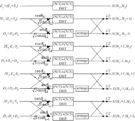
So far, we have decomposed a length-N×N DHT (defined in (1)) into nine length-(N/3)×(N/3) DHTs (defined in (8) through (16)). Fig. 1 shows the flowgraph of the realization of the proposed algorithm.

III. COMPUTATIONAL COMPLEXITY AND COMPARISON ANALYSIS

In this section, we consider the computational complexity of the proposed algorithm and compare it with some known algorithms. The detailed analysis is given below.

i) The computation of (4) and (5) requires (N/3)×(N/3)×14 additions.

ii) The implementation of the butterfly in the input data sequence of Ai(k1, k2) and Bi(N/3–k1, N/3–k2), i = 1, 2, 3, 4,

needs 4 multiplications and 2 additions, thus, the computation from (8) to (16) requires (N/3)×(N/3)×16 multiplications and (N/3)×(N/3)×25 additions.

iii) The computation of X(k1, k2) from Ai(k1, k2), i = 0, 1, 2, 3, 4,

and Bi(k1, k2), i = 1, 2, 3, 4, requires (N/3)×(N/3)×8

additions.

iv) Taking the special cases n1 = 0, n2 = 0, n1 + n2 = 0 or N/3,

and n1 = n2 into consideration, 4N multiplications and 2N+2

additions can be saved in the computation through (8) to (16). In fact, let us consider, for example, the number of arithmetic operations that can be saved in the computation of (13) and (14) for the cases where n1 + n2 = 0 or N/3.

Letting a11 = 2E3–E4–S3 and b11 = D1+D2–D3, when n1 +

n2 = 0, the input data sequences in (13) and (14) become a11

and 3b₁₁, in such case, 3 multiplications and 2 additions can be saved. When n1 + n2 = N/3, the input data sequences

become ( _{11 11}) 2 ₁₁ 2 1 b b a − − − and ( ) 2 3 11 11 b a − ⎪⎩ ⎪ ⎨ ⎧ + − − = + − = × × × × , 9 2 2 9 / 47 , 9 4 9 / 16 ) 3 / ( ) 3 / ( 2 ) 3 / ( ) 3 / ( 2 N N N N N N N N A N N A M N N M , N–3 multiplications can be saved. Therefore, for the two cases n1 + n2 = 0 and n1 + n2 = N/3, N multiplications and 2

additions can be saved in the computation of (13) and (14). A similar analysis can be done for other cases.

The computational complexity of the proposed algorithm is therefore given by

(17) with initial values M3×3 = 4 and A3×3 = 47.

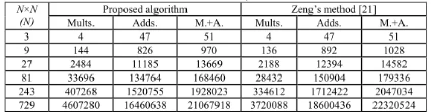
Table I shows the computational complexity required by the proposed algorithm and Zeng’s method [21] for the block size 3m_×3m_{, m≥1. Tables II and III present the computational}

complexities of Zeng’s approach [22] and Bi’s algorithm (q = 1) [9], [10] for the block size 2m×2m, m ≥ 2 and Bi’s algorithm (q = 3) for the block size 3*2m_×3*2m_{, m ≥ 0, respectively. Note that}

in Bi’s algorithm for q = 3, the same initial values M3×3 = 4 and

A3×3 = 47 are used. To make the comparison more clear, Fig. 2

shows the number of multiplications plus additions, involved in the computation of the length-N×N DHT, using the proposed method and the algorithms presented in [9], [10], [21] and [22]. It can be seen from Table I that the proposed algorithm is more efficient than Zeng’s method [21] in terms of the total number of arithmetic operations. Tables II and III, as well as Fig. 2, show that the proposed algorithm is more efficient, in some cases, than the algorithms presented in [9], [10], and [22] in terms of the number of arithmetic operations, especially for the cases where there is many zero padding, such as block sizes 9×9 and 81×81. Thus, user may favor a given technique depending on the selected block size. For more detailed discussion about the vector-radix algorithm and the polynomial algorithm, we refer the readers to Ref. [16].

IV. CONCLUSIONS

We have proposed in this paper a radix-3×3 DIF algorithm for the fast computation of 2-D DHT. Compared with some known algorithms, the proposed one achieves substantial saving on the number of arithmetic operations. Moreover, the proposed algorithm possesses properties such as the butterfly-style and in-place computations that are highly

l q1×

desirable for software as well as hardware implementation. It can be used for fast convolution where one uses the minimum block sizes compatible to the filter specifications. Note that our radix-3×3 algorithm can be easily extended to the arbitrary radix-q×q case, where q is an odd integer, which provides a wider choice of block sizes. Thus, user can favor an approach for a desired block. Furthermore, our proposed algorithm, combing with other split vector-radix algorithms [5-10], can realize the 2-D DHT with block size 3m₂n_×3m₂n_{, m, n ≥ 2. Since}

the DHT is an efficient alternative to the DFT for real data, the proposed algorithm may also find its application in array signal processing [25].

[18] W. Ma, “Algorithm for computing two-dimensional discrete Hartley transform of size pn_×pn_{,” Electron. Lett., vol. 26, no. 21, pp. 1795-1797,}

Oct. 1990.

[19] W. Ma, “Number of multiplications necessary to compute length-2n

two-dimensional discrete Hartley transform DHT (2n_{; 2),” Electron. Lett.,}

vol. 28, no. 5, pp. 480-482, Feb. 1992.

[20] S.C. Chan and K.L. Ho, “Polynomial transform fast Hartley transform,”

IEEE ISCAS, vol. 1, Jun. 1991, pp. 642-645.

[21] Y. H. Zeng, G. Bi, and A. C. Kot, “Fast algorithm for multi-dimensional discrete Hartley transform with size _ql2_×"×qlr_{,” Signal Process.,}

vol. 82, no. 3, pp. 497-502, Mar. 2002.

[22] Y. H. Zeng, G. Bi, and A. R. Leyman, “New algorithms for multidimensional discrete Hartley transform,” Signal Process., vol. 82, no. 8, pp. 1086-1095, Aug. 2002.

[23] E. Dubois and A.N. Venetsanopoulos, “A new algorithm for the radix-3 FFT,” IEEE Trans. Acoust., Speech, Signal Process., vol. 26, no. 3, pp. 222-225, Jun. 1978.

[24] Z.J. Zhao, “In-place radix-3 fast Hartley transform algorithm,” Electron.

Lett., vol. 28, no.3, pp. 319-321, Jan. 1992.

REFERENCES _{[25] C.J. Ju, “Algorithm of defining 1-D indexing for M-D mixed radix FFT} implementation,” IEEE PRCCCSP, vol.2, May 1993, pp. 484-488. [1] R.N. Bracewell, The Hartley Transform, New York, NY: Oxford Univ.

Press, 1986.

[2] I. Duleba, “Hartley transform in compression of medical ultrasonic

images,” Proc. IEEE ICIAP, Sept. 1999, pp. 722-727. Table I The computational complexity required by the proposed algorithm and Zeng’s

method for the block size 3m_×3m_{, m≥1}

[3] N.C. Hu and F.F. Lu, “Fast computation of the two-dimensional generalised Hartley transforms,” IEE Proc. Vis. Image Signal Process., vol. 142, no.1, pp. 35-39, Feb. 1995.

N×N

(N) Mults. Adds. M.+A. Mults. Adds. M.+A. Proposed algorithm Zeng’s method [21] 3 4 47 51 4 47 51 9 144 826 970 136 892 1028 27 2484 11185 13669 2188 12394 14582 81 33696 134764 168460 28432 150904 179336 243 407268 1520755 1928023 334612 1712422 2047034 729 4607280 16460638 21067918 3720088 18600436 22320524

[4] R.N. Bracewell, O. Buneman, H. Hao, and J. Villasenor, “Fast two-dimensional Hartley transform,” Proc. IEEE, vol. 74, no. 9, pp. 1282-1283, Sept. 1986.

[5] R. Kumaresan and P.K. Gupta, “Vector-radix algorithm for a 2-D discrete Hartley transform,” Proc. IEEE, vol. 74, no. 5, pp. 755-757, May 1986. [6] E.A. Jonckheere and C. Ma, “Split-radix fast Hartley transform in one and

two dimensions,” IEEE Trans. Signal Process., vol. 39, no.2, pp. 499-503,

Feb. 1991. Table II The computational complexity needed by Zeng’s approach and Bi’s _{algorithm (q=1) for the block size 2}m_×2m_{, m≥2}

[7] S. Huang, J. Wang, and H. Qiu, “Split vector radix algorithm for two-dimensional Hartley transform,” IEEE Trans. Aerosp. Electron. Syst. vol. 27, no.6, pp. 865-868, Nov. 1991.

N×N (N)

Zeng’s approach [22] Bi’s algorithm (q=1) [9][10] Mults. Adds. M.+A. Mults. Adds. M.+A. 4 2 58 60 2 58 60 8 26 354 380 24 408 432 16 218 2018 2236 264 2216 2480 32 1370 10594 11964 1800 11368 13168 64 7514 52578 60092 10536 55176 65712 128 38234 251234 289468 55560 260840 316400 256 185690 1168738 1354428 277992 1200712 1478704 512 873818 5330274 6204092 1333320 5443368 6776688 1024 4019546 23942498 27962044 6232872 24305288 30538160

[8] J.L. Wu and S.C. Pei, “The vector split-radix algorithm for 2D DHT,”

IEEE Trans. Signal Process., vol. 41, no.2, pp. 960-965, Feb. 1993.

[9] G. Bi, “Split-radix algorithm for 2-D discrete Hartley transform,” Signal

Process., vol. 63, no. 1, pp. 45-53, Nov. 1997.

[10] G. Bi, A.C. Kot, and Z. Meng, “Computation of 2D discrete Hartley transform,” Electron. Lett., vol. 34, no.11, pp. 1058-1059, May 1998. [11] S. Boussakta, O.H. Alshibami, and M.Y. Aziz, “Radix-2×2×2 algorithm

for the 3-D discrete Hartley transform,” IEEE Trans. Signal Process., vol. 49, no. 12, pp. 3145-3156, Dec. 2001.

[12] O. Alshibami and S. Boussakta, “Fast 3-D decimation-in-frequency algorithm for 3-D Hartley transform,” Signal Process., vol. 82, no. 1, pp. 121-126, Jan. 2002.

Table III The computational complexity needed by Bi’s algorithm (q=3) for the block size 3*2m_×3*2m_{, m ≥ 0}

N×N

(N) Mults. Bi’s algorithm (q=3) [9][10]Adds. M.+A.

3 4 47 51 6 16 260 276 12 64 1328 1392 24 472 6680 7152 48 3400 31976 35376 96 20296 150440 170736 192 111208 689096 800304 384 565576 3117608 3683184 768 2764072 13886600 16650672

[13] S. Bouguezel, M.O. Ahmad, and M.N.S. Swamy, “An efficient three-dimensional decimation-in-time FHT algorithm based on the radix-2/4 approach,” Proc. IEEE ISSPIT, Dec. 2004, pp. 52-55.

[14] S. Bouguezel, M.O. Ahmad, and M.N.S. Swamy, “A split vector-radix algorithm for the 3-D discrete Hartley transform,” IEEE Trans. Circuits

Syst.-I: Regular paper, vol. 53, no. 9, pp. 1966-1976, Sept. 2006.

[15] S. Bouguezel, M.O. Ahmad, and M.N.S. Swamy, “An efficient multidimensional decimation-in-frequency FHT algorithm based on the radix-2/4 approach,” IEEE ISCAS, May 2005, pp. 2405-2408.

[16] S. Bouguezel, M.N.S. Swamy, and M.O. Ahmad, “Multidimensional vector radix FHT algorithms,” IEEE Trans. Circuits Syst.-I: Regular

paper, vol. 53, no. 4, pp. 905-917, Apr. 2006.

[17] D. Yang, “New fast algorithm to compute two-dimensional discrete Hartley transform,” Electron. Lett., vol. 25, no. 25, pp. 1705-1706, Dec. 1989.

Fig. 1. Radix-3×3 algorithm for the 2-D DHT “arrange” means the time-reversal operation of the sequence

3 9 27 81 243 729 102 103 104 105 106 107 Block size(N×N) T he n um ber of m ul ti pl ic a ti ons pl us a ddi ti ons Proposed algorithm Zeng's method Zeng's approach Bi's algorithm(q=1) Bi's algorithm(q=3) 51 (N)

Fig.2. Comparison among the proposed algorithm, Bi’s algorithm and Zeng’s algorithm in terms of multiplications plus additions.