Continuous and Non-invasive Blood Pressure
Monitoring using Ultrasonic Methods
by
MASSACHUSETTS INS EOF TECHNOLOGY
Joohyun Seo
JUN 10 2014
B.S. in Electrical Engineering
Seoul National University (2012)
LIBRARIES
Submitted to the Department of Electrical Engineering and Computer
Science
in partial fulfillment of the requirements for the degree of
Master of Science in Electrical Engineering and Computer Science
at the
MASSACHUSETTS INSTITUTE OF TECHNOLOGY
June 2014
@
Massachusetts Institute of Technology 2014. All rights reserved.
Signature redacted
Author ...
o E
r
Enginering.ad.omS...
Department of Electrical Engineering and Computer Science
Certified by...
Signature redacted
May 21, 2014
Hae-Seung Lee
ATSP Professor of Electrical Engineering
Certified by.
Signature redacted
Thesis Supervisor
Charles G. Sodini
Lebel Professor of Electrical Engineering
Accepted by ...
Signature redacted
Le
Thesis Supervisor
...
shie A. Kolodziejski
Chair, Department Committee on Graduate Students
Continuous and Non-invasive Blood Pressure Monitoring
using Ultrasonic Methods
by
Joohyun Seo
Submitted to the Department of Electrical Engineering and Computer Science on May 21, 2014, in partial fulfillment of the
requirements for the degree of
Master of Science in Electrical Engineering and Computer Science
Abstract
This thesis presents a continuous and non-invasive arterial blood pressure (CNAP) monitoring technique using ultrasound. An arterial blood pressure (ABP) waveform provides valuable information in treating cardiovascular diseases. Although aii inva-sive ABP measurement through arterial catheterization performed in an inteninva-sive care unit (ICU) is considered a gold standard, its invasive nature not only increases various patients' risks but makes its usage for cardiovascular studies expensive. Therefore, reliable non-invasive ABP waveform estimation has been desired for a long time by medical communities.
This work details ABP waveform estimation based on a vessel cross-sectional area measurement combined with the elastic property of an arterial vessel, represented
by a pulse wave velocity (PWV). Several ultrasound techniques including uniform
insonation and echo-tracking are explored to measure the PWV using so-called QA method as well as the cross-sectional area. The physiological background of the arterial system and considerations for a clinical test are also presented.
Experimental results validate the QA method and the proposed ABP waveforn es-timation method in a custom-designed experimental setup consisting of a diaphragm pump and a latex rubber tube using two commercially available single element ul-trasonic transducers. The design of a portable CNAP monitoring device using ultra-sound will fuel the exponential growth of a readily available, inexpensive but powerful cardiovascular diagnostic tool.
Thesis Supervisor: Hae-Seung Lee
Title: ATSP Professor of Electrical Engineering Thesis Supervisor: Charles G. Sodini
Acknowledgments
First of all, I would like to appreciate my parents for their endless support on my academic journey at the MIT. Certainly, starting a new research project in a foreign country was not smooth, but their emotional support and faith on me as a student and their son have motivated me greatly to complete this Master's thesis. As always, they have been great mentors in my life, and they will be in the future as well.
I would like to express my greatest appreciation to research advisors, Professors
Hae-Seung Lee and Charles Sodini. Their exceptional insight and extensive technical knowledge always guide me in the right direction. Besides, their mentorship and advices help me realize and become a better student and researcher. Without their technical guidances, this thesis work could not be completed.
Next, technical advices from Dr. Kai Thomenius (MIT) regarding medical ul-trasound have been particularly helpful. His extraordinary knowledge in medical ultrasound helps me increase the depth of this thesis. Also, I would like to thank Dr. Brian Brandt (Maxim Integrated) for his generous interest on this work and for the opportunity of me giving a talk at the Maxim Integrated Boston design center. I also appreciate insightful comments from Dr. Toni O'Dwyer (Analog Devices) from weekly meetings.
Lastly, I thank all my colleagues in 38-265 for me to enjoy delightful office life.
Especially, Sabino Pietrangelo and Dr. Kailiang Chen has helped me troubleshoot hardware issues and resolve any difficulties encountered on my research. The con-structive discussion with other colleagues on various topics also expands my scope of knowledge not only in medical ultrasound and medical electronics, but also in analog circuit designs and beyond.
This work is partially funded by the MIT Center for Integrated Circuits and Systems (CICS). In addition, Samsung fellowship is appreciated for financial support on my graduate student life at the MIT.
Contents
1 Introduction 15
1.1 Cardiovascular Disease Diagnostics . . . . 15
1.2 M otivation . . . . 17
1.3 Objective of Thesis Work . . . . 19
1.4 Thesis Organization . . . . 20
2 General Ultrasound Background 21 2.1 Acoustic Wave in Tissue . . . . 21
2.1.1 Acoustic Wave Propagation . . . . 21
2.1.2 Acoustic Wave Scattering . . . . 23
2.2 Ultrasonic Transducer Characterization . . . . 30
2.2.1 Piezoelectric Element Physics . . . . 30
2.2.2 Equivalent Circuit Model . . . . 32
2.2.3 Pressure Field in Continuous Wave . . . . 34
2.2.4 Pressure Field in Pulsed Wave . . . . 37
3 Hemodynamics of Arterial System 41 3.1 Blood Flow Physics . . . . 41
3.1.1 Steady Flow . . . . 42
3.1.2 Pulsatile Flow . . . . 44
3.2 Pulse Pressure Wave . . . . 46
3.2.1 Pulse Pressure Wave Propagation . . . . 47
3.3 Anatomical and Physiological Background of Arterial System . . .. . 5
4 Arterial Blood Pressure Waveform Estimation Technique 55 4.1 Pulse W ave Velocity . . . . 55
4.2 Blood Flow Estimation . . . . 58
4.2.1 Doppler Ultrasound Theory for a Single Scatterer . . . . 58
4.2.2 Volumetric Flow Rate . . . . 63
4.3 Vessel Cross-Sectional Area Estimation . . . . 69
5 Experimental Test 5.1 Experimental Setup . . . . 5.1.1 Flow Phantom Characterization . . 5.1.2 Ultrasound System . . . . 5.1.3 Pressure Sensor . . . . 5.2 Experimental Procedure . . . . 5.3 Experimental Results . . . . 5.3.1 Pressure Sensor Calibration . . . . 5.3.2 Flow Velocity Measurement . . . . 5.3.3 Pulse Wave Velocity Measurement 5.3.4 Pressure Waveform Comparison . . 77 . . . . 77 . . . . 77 . . . . 80 . . . . 8 1 . . . . 8 2 . . . . 84 . . . . 84 . . . . 8 5 . . . . 87 . . . . 94 6 Conclusion 6.1 Summary . . . . 6.2 Future Work. . . . . 97 97 98 51
List of Figures
2-1 Oblique incident wave on a boundary between media with different
acoustic im pedances . . . . 25
2-2 Specular scattering of a planar incident wave on a spherical object . 26
2-3 Diffusive scattering of a planar incident wave on a spherical object . 27
2-4 Diffusive Scattering of an incident wave on scattering volume from [18] 28
2-5 Piezoelectric element with parallel electrodes . . . . 30
2-6 KLM equivalent circuit model for a piezoelectric element . . . . 32
2-7 Geometric representation of a transducer aperture and its coordinates 35
2-8 Simulated continuous pressure in a radial axial dimension for a circular
aperture of 5 mm radius at continuous 2 MHz ultrasound . . . . 36
2-9 Simulated continuous pressure a temporal-averaged intensity field in
x - z and x - y plane for a circular aperture of 5 mm radius at 2 MHz
ultrasound . . . . 37
2-10 Simulated pulsed pressure a temporal-averaged intensity field in x - z
and x - y plane for a circular aperture of 5 mm radius at 3 cycles of 2
M H z ultrasound . . . . 39
3-1 Illustration of force on small fluid volume in a rigid tube from [15] . . 43
3-2 Illustration of Womnersley's pulsatile velocity profile in different cardiac
p h ases . . . . 46
3-3 Schematic of an clastic tube . . . . 47
3-4 Pressure (above) and blood flow velocity (below) of arteries in a dog
3-5 Illustration of vascular structures in upper body from [28] . . . . 52
3-6 Illustration of vascular structures in the neck from [29] . . . . 53
3-7 Illustration of vascular structures in upper arm from [29] . . . . 54
4-1 Diagram of pulsed Doppler time compression from [15] . . . . 59
4-2 Direct sampling for the single range gate of pulsed Doppler ultrasound 61 4-3 Relationship between the round trip time delay in pulsed Doppler and the frequency shift due to the Doppler effect . . . . 62
4-4 Illustrated series of small sample volumes defined along cross-section to measure a complete velocity profile . . . . 64
4-5 Illustration of an uniform insonation approach . . . . 65
4-6 Illustration of a velocity profile in different poiseuille profiles . . . . . 66
4-7 Simulation of an overestimated spatial mean velocity in 6.26 mm vessel depending on -3dB beam width . . . . 66
4-8 Simulation of spatial mean velocity estimate error with the different SNR of a moving scatterer signal in Doppler spectrum . . . . 67
4-9 Simulation of a spatial mean velocity estimate variation in a parabolic velocity profile . . . . 68
4-10 Illustration of multiple spatial mean velocity estimates in an uniform insonation . . . . 69
4-11 Simulation of an averaged spatial mean velocity estimate of seven ve-locity waveforms from seven sample volumes . . . . 69
4-12 Simulated echo with a threshold function set by sustain attack filter approach... ... 72
4-13 Simulated performance comparison of echo shift estimators for vessel wall velocity estim ation . . . . 74
4-14 Simulation of an estimated diameter change over sixteen cardiac cycles using the C3M estimator . . . . 75
5-2 Measured power spectral density of pressure waveform in constant
pum p supply voltage . . . . 79
5-3 Two ultrasonic transducers configuration . . . . 80 5-4 Two channel signal processing block diagram . . . . 82 5-5 Illustration of signal processing flow from raw physiological waveforms
to pressure waveform . . . . 83
5-6 Measured sensitivity of a pressure sensor . . . . 85 5-7 Spatial mean velocity measurement using an uniform insonation . . . 86 5-8 Measured spatial mean flow velocity in periodic pulsatile flow . . . . 87
5-9 Wall-lumen interface identification using sustain-attack filter approach from the envelop of a measured echo . . . . 88 5-10 Measured pulsatile diameter waveform in periodic pulsatile flow . . . 89 5-11 Measurement of the typical supply voltage waveform of the pump . . 89 5-12 Measurement of a typical flow-area plot . . . . 90 5-13 Comparison of averaged pressure waveforms from 1) ultrasonic
meth-ods and 2) pressure sensor measurement . . . . 91
5-14 Pulse wave velocity estimation statistics . . . . 92 5-15 Measured flow-area plots in various pulsatile frequencies . . . . 93 5-16 Measured flow-area plot in different observation sites along a latex
rubber tube ... ... 94
5-17 Measured pressure waveform comparison in different pressure
List of Tables
2.1 Acoustic parameters in biological media from [15,16] . . . . 23
2.2 Relative magnitude of scattered acoustic wave in biological tissues from
[1 6 ] . . . . 2 9
3.1 Analogy of pulse pressure propagation in elastic tube to transmission
Chapter 1
Introduction
1.1
Cardiovascular Disease Diagnostics
The world health organization (WHO) defines cardiovascular diseases (CVD) as a
group of disorders of the heart and blood vessels. CVDs include coronary heart
disease, cerebrovascular disease, peripheral arterial disease, rheumatic heart disease, congenital heart disease, deep vein thrombosis and pulmonary embolism. CVDs re-lated to the heart muscle and the brain are critical because these organs are vital to maintain life. According to the report from the WHO, CVDs are the leading cause of death. The WHO report estimates that 17.3 million people died from CVDs in 2008, which accounts for 30% of global deaths [1]. Of the 17.3 million deaths, the report estimates that 7.3 million were due to the coronary heart disease (i.e., the CVD of the artery supplying blood to the heart muscle), and 6.2 million cases were due to stroke (i.e., the loss of brain function due to reduced blood supply). According to the WHO fact sheets, hypertension accounts for 9.4 million deaths annually, and this figure includes 51% of deaths caused by the stroke and 45% by the coronary heart disease. Since the stroke and heart attack are acute and generally life-threatening, a significant amount of research has been conducted to identify a risk factor for these diseases.
In general, the study of the human circulatory system is of great importance be-cause it delivers oxygen and nutrition as well as removes carbon dioxide and waste
to sustain metabolism and respiration. For CVD studies and diagnosis, various tools
have been developed, validated and clinically accepted. For example, an electrocardio-gram (ECG; recordings of body surface potential) assesses the electrical functionality of the heart, which is depolarization followed by repolarization as the atria and ventri-cles successively contract. Because of its non-invasive and practical nature, the ECG signal has been broadly used in both ambulatory, and at the bedside. The normal
ECG signal features P wave followed by the QRS complex and T wave successively,
and the interpretation of the signal is well established for cardiologists to diagnose various heart diseases (e.g., ventricular tachycardia, ventricular fibrillation) and to make clinical decisions in a timely manner.
Also, the anatomy of the vascular system has been studied in a non-invasive man-ner with the help of various imaging modalities such as ultrasonography, computed tomography (CT), angiography and magnetic resonance imaging (MRI). Doppler spectrogram is another good example of a clinically accepted diagnostic technique to examine the circulatory function. The Doppler spectrogram measures blood flow velocity based on the Doppler effect of an acoustic wave. With the spectrogram, physicians and sonographers diagnose vascular diseases such as arteriosclerosis or measure cardiac output (i.e., blood volume pumped by the heart for one minute).
Finally, blood pressure, more often referred to as arterial blood pressure (ABP), is a key physiological parameter in assessing the circulatory system. Oftentimes, the blood pressure is measured by a sphygmomanometer with an inflatable cuff wrapped around the upper extremity. At the beginning of measurement, the cuff occludes the brachial artery completely and release pressure until the artery just starts open at the systolic stage to measure systolic blood pressure. Then, it continues to re-lease pressure until the artery remains open for an entire cardiac cycle to measure diastolic blood pressure. Because of the simplistic usage and non-invasive nature, the sphygmomanometer became a primary instrument to measure blood pressure. However, it produces only systolic and diastolic blood pressure measurements at one moment, which are highly undersampled measurements in time and insufficient to truly represent the dynamic behavior of the cardiovascular system.
A complete ABP waveform is only available in an intensive care unit (ICU) of
hospitals. On heavily monitored ICU patients, the radial or the femoral artery is accessed through arterial catheterization. This procedure provides a pathway to ad-minster drugs directly to the arterial system, instead of intravaneous methods, to collect an arterial blood sample for laboratory tests such as arterial blood gas and to measure the ABP waveform. A pressure sensor connected via a rigid tubing to an arterial catheter directly reads the ABP waveform although a pressure wire is occa-sionally inserted to obtain the ABP waveform at different arterial sites. The ABP waveform truly reflects hemodynamic phenomena, and the waveform itself is a rich source of information for CVD research.
1.2
Motivation
The ABP waveforn provides valuable information of the circulatory system of pa-tients. By analyzing the ABP waveform, a powerful predictor for CVDs is often found. For example, high pulse pressure (PP; difference between systolic and dias-tolic blood pressure) was reported as a risk factor for the coronary heart disease in
the middle-aged and elderly
[2].
Similarly, the pulsatility of ascending aortic pressurewas found as a strong predictor for recurrence of stenosis (i.e., narrowing of blood
vessel) after percutaneous transluninal coronary angioplasty [3].
In addition, various physiological parameters derived from the ABP waveform not only assist hospital staff to make clinical decisions but allow them to navigate compli-cated relations between hemodynamics parameters. For instance, a continuous car-diac output (CO) monitoring method using a peripheral ABP waveform was proposed and verified with a swine experiment [4]. Following this study, monitoring continu-ous CO and total peripheral resistance (TPR) over varicontinu-ous ambulatory activities was introduced [5]. In addition to these studies, an adaptive transfer function to derive a central ABP waveforn from the peripheral ABP waveform was proposed to find a better indicator for hemmorhage, which potentially benefits battlefield medicine [6]. These examples testify indispensability of the ABP waveform in cardiovascular
re-search.
Unfortunately, the ABP waveform is typically obtained only through the arterial catheterization as mentioned previously. Although considered a gold standard, the disadvantage of this method is its invasive nature. This invasive nature unavoidably increases the possibility of infection through the artery as well as damage to adjacent tissue because the artery usually lies deep below the skin. The anticipated patients' risks tend to confine the usage of the ABP waveform obtained by arterial catheteri-zation in critical-care decisions. In addition, the ABP waveform is used limitedly in cardiovascular research because the waveform is not readily obtainable.
Currently, some non-invasive ABP waveform monitoring techniques have been introduced to overcome the limitation of the gold standard method, and they fall mainly into two categories: arterial tonometry and a volume clamp. The arterial tonometry is a transcutaneous pulse sensing technique to directly determine the blood pressure inside an artery. A tonometer applies enough pressure to distort the vessel until normal contact stress between the skin and the tonometer surface becomes the same as blood pressure [7]. In general, tonometry requires a superficial artery with a desirable size supported by a hard structure such as bones. Because of this requirement, tonometry cannot be applied to all patients and arterial sites [8]. For example, the quality of the pressure measurement from obese patients is poor. In
addition, the measurement at femoral artery using applanation tonometry was found unreliable in a large number of subjects [8].
The volume clamp type is based on the method reported by Penaz [9]. This type of device applies external pressure with an inflatable finger cuff while measuring blood volume through an infrared photoplethysmograph. Blood volume measured by the plethysmograph is clamped by adjusting the cuff pressure to match the blood pressure change, and the cuff pressure is read as the blood pressure measurement [10]. A volume clamp point is set to make the artery only partially occluded to keep reasonable oxygenation level of the finger tip. The accuracy of this device has been investigated in articles to compare it to intra arterial blood pressure recording [10,11]. Also, this type of device was also utilized to obtain the peripheral ABP waveform [5,6].
Although the performance of the device continues to improve, it only measures the
finger ABP waveform and requires the cuff, thus lessening patients' comfort for long term monitoring with reduced blood flow to the finger tip.
In order to overcome some of these limitations, ultrasonography appears as a viable
option because it is a promising non-invasive imaging modality in investigating both vascular anatomy and hemodynamics of patients. Compared to other modalities, such as CT and MRI, medical ultrasound is far less expensive, free of radiation and poten-tially suitable to portable system implementation. Because of these benefits, medical ultrasound has already been widely adopted for daily screening, subcutaneous tissue structure imaging and medical diagnostics such as obstetric sonography. Therefore, the ABP waveform monitoring using ultrasound is a particularly intriguing research issue not only because of its non-invasive nature but because of its cost efficiency and potential aptness for a portable medical device. Additionally, an ultrasound approach eliminates the necessity for the inflatable cuff, thereby promoting patients' comfort desirable for long-term monitoring.
1.3
Objective of Thesis Work
The main objective of this thesis work is to address the ABP waveform estimation technique using physiological waveforms obtained by various ultrasound techniques and to experimentally verify the effectiveness of the technique. The following six aims detail the main objective:
" Background
- To provide background in medical ultrasonography
- To describe the behavior of the ABP waveform in the human arterial sys-tem on the basis of hemodynamics
" Experimental Validation
- To estimate flow velocity using pulsed Doppler ultrasound.
- To estimate a local pulse wave velocity using physiological waveforms - To estimate a pressure waveform and compare it with a reference waveform. Additionally, this thesis work lays the ground work for a future clinical test of the ABP waveform estimation.
1.4
Thesis Organization
This thesis begins with general ultrasound background in Chapter 2. This chapter describes the propagation of an acoustic wave, scattering mechanisms which essen-tially allow diagnostic ultrasound to work. Chapter 2 continues with acoustic wave generation in a piezoelectric element and its equivalent circuit model followed by the description of acoustic pressure field patterns in both continuous and pulsed waves.
The anatomical background of the human arterial system relevant to the ABP measurement is described in Chapter 3. This chapter proceeds to blood flow physics and the relationship between physiological parameters such as blood pressure and blood flow. Finally, the behavior of a pulse pressure wave and its propagation speed are analyzed within a simplified elastic tube model.
In Chapter 4, a method to estimate ABP waveform is first described with neces-sary physiological waveforms: a spatial mean blood velocity and an artery diameter waveform. Several ultrasound methods are introduced and compared with each other. Their benefits and limitations in estimating the physiological waveforms are discussed. The experimental results of the pressure waveform estimating technique is pre-sented in Chapter 5. This chapter characterizes a custom designed experimental setup and explains experimental procedures. The experimental results begin with pressure sensor calibration, spatial mean velocity estimation, local pulse wave ve-locity estimation followed by the verification of the pressure waveform estimation. Chapter 6 discusses the key contribution of this thesis work and addresses future works.
This thesis includes many results of acoustic field simulation conducted in Field II ultrasound simulation program [12,13].
Chapter 2
General Ultrasound Background
This chapter describes a basic theory of operation of ultrasonography. The ultrasonog-raphy is an imaging or diagnostic technique using ultrasound which is defined as a longitudinal acoustic wave above audible frequencies. This chapter gives a theoretical view mainly in two aspects: an acoustic wave theory and ultrasound transducer de-sign and characterization. The following section defines variables in the acoustic wave theory and describes the interaction of the acoustic wave with tissue via absorption and scattering.
2.1
Acoustic Wave in Tissue
2.1.1
Acoustic Wave Propagation
An acoustic wave can propagate through all phases of matter: gas, liquid and solid, and the propagation mode nay differ from phase to phase. In diagnostic ultrasound, the analysis of acoustic wave propagation in water sets basis because the acoustic characteristics of tissue, which mainly consists of water, is fairly similar to that of water. Although the exact characterization of tissue as a muedium also involves non-linearity and complicatedness, a linear analysis iii water provides an insight of the overall wave behavior. Additionally, only the longitudinal wave exists in water, which keeps the analysis simple [14].
The following analytics is based on the assumption that the medium is an idealized
inviscid fluid [14]. As the acoustic wave propagates, particles in the medium are
displaced from its resting position in an oscillatory manner. The displacement results in local pressure disturbance as a result of the compression and expansion of the medium. A particle velocity (v) is expressed as, by definition,
t(),
t) = at' (2.1)
where u is a displacement. For convenience of analysis, a velocity potential (#) is defined as
v(IF, t) = V#(i, t) (2.2)
Then, a pressure (p) is defined in terms of the velocity potential as
p(j?, t) = -POO(I t)
('1 0at
(2.3)where p is the density of fluid at rest. An acoustic wave equation is written in three dimensional space as
1
a
2q5(i?
t)V20(, t) _ 20-
a2
t
2
t2)= 0 (2.4) where c is the speed of sound. The speed of sound is determined by properties of themedium which are the isothermal bulk modulus (BT), the ratio of specific heats (7)
and the density (p).
C = (2.5)
p
The solution of the wave equation indicates two waves traveling in forward and back-ward direction. A specific acoustic impedance is defined as the ratio of pressure to the particle velocity in a forward traveling wave. The acoustic impedance has a unit
of kg/n 2 .
s, also known as Rayls. Typical acoustic parameters of water, tissue and blood are summarized in Table 2.1.
An instantaneous intensity (Jinst) is expressed in terms of the acoustic impedance
as:
Table 2.1: Acoustic parameters in biological media from [15,16]
.u Density Acoustic Impedance Speed of Sound
(kg/m 3) (MRayls) (m/s)
Air 1.2 0.0004 333
Water 998 1.48 1481
Blood 1060 1.66 1566
Soft Tissue (average) 1058 1.63 1540
Iinst = p(ft)p*(, t) =
z
v(r, t)v*(f, t)Z (2.7)Instead of the instantaneous intensity, an averaged intensity in either a temporal or a spatial domain delivers the clear view of acoustic energy transfer. Also, the intensity is certainly an essential parameter in safety consideration [17]. A spatial-average (SA) intensity provides the sense of total power generated by an ultrasonic transducer while a spatial-peak (SP) intensity or maximum intensity is more pertinent to the safety. Meanwhile, a temporal-average (TA) intensity results in the spatial pattern of an acoustic field, and this pattern, also known as a beam pattern, is important in
diagnostic ultrasound because the beam pattern is not usually uniform in the region of interest. The usage and performance of an ultrasound system relies on defining the desirable beam pattern, which is typically evaluated in terms of the TA intensity. In case the acoustic wave is pulsed, a pulse-average (PA; average over pulse cycles) intensity is also used as a substitute for the TA intensity [17].
2.1.2 Acoustic Wave Scattering
An acoustic wave gradually loses its energy as it propagates through biological tissues. This energy loss is mainly attributed to two phenomena: absorption and scattering
[18]. A plane wave attenuated as it travels is expressed as:
where a is known as an attenuation coefficient. The exact attenuation coefficient changes among various tissues and also increases as the frequency of the acoustic wave rises. The dependency of the attenuation coefficient on frequency comes from stronger diffusive scattering at a higher frequency, which is discussed in the following
paragraphs. Typically, the attenuation coefficient in soft tissue is 1 dB/cm at 2
MHz [17].
Absorption in tissue usually refers to energy transfer from acoustic energy to other forms of energy such as heat. Therefore, the safety regulation of diagnostic and therapeutic ultrasound ensures to prevent tissue damage caused by excessive heating. The acoustic scattering not only weakens the propagating wave but, most importantly, makes the acoustic wave return and excite the ultrasonic transducer so that hospital staff can interpret a detected signal to diagnose patients.
The scattering occurs when the acoustic wave propagates through inhomogeneous medium and results in radiating secondary waves. Three types of the scattering mech-anism exist, and the mechmech-anism at the medium boundary is categorized depending on the dimension or roughness of the boundary relative to the wavelength of the incident acoustic wave: specular scattering (i.e., reflection), diffusive scattering and diffractive scattering [14].
Specular Scattering
The specular scattering occurs when the roughness of an object or the boundary is much greater than the wavelength of the acoustic wave, and it can be simply un-derstood as reflection. A ray theory is sufficient to explain the trajectories of both a reflected and a transmitted wave as shown in Figure 2-1. In biological tissue, the boundary of organs, bones and other macro structures falls into this type. By solving boundary conditions, which states that the pressure and the particle velocity are con-tinuous, and tangential components of wavenumbers match, the angle of transmission
1 Z1, Ci Reflected Wave OR Oi Incident Wave 2 Z, C2 Transmitted Wave
Figure 2-1: Oblique incident wave on a boundary between media with different acous-tic impedances
sin 01 c1
sin OT C2
(2.9)
where ci and c2 are the speed of sound in medium 1 and 2, respectively. At the same
time, the angle of reflection (OR) is equal to the angle of incidence (0j) dictated by
the ray theory. Since the wavenumber component normal to the boundary has cosine dependency, effective acoustic impedances of medium 1 and 2 are expressed as
Zior pic1 _ Zl cos0 1 -cosO 1 Z20T p2c2 _ Z2 cosOT - cosOT (2. 10a) (2. 10b)
where p1 and P2 are the density of medium 1 and 2,' respectively. As a result, a
reflection factor (RF) and a transmission factor (TF) are given by:
Z20T - Z 101 Z2 cos 01 - Z1 cos OT Z20T + Z 10 1 Z2 cos 01 + Z1 cos OT TF~ 2Z29T 2Z2 cos 01 Z20T + Z10, Z2cos 01 + Z1 cos OT (2.11a) (2.11b)
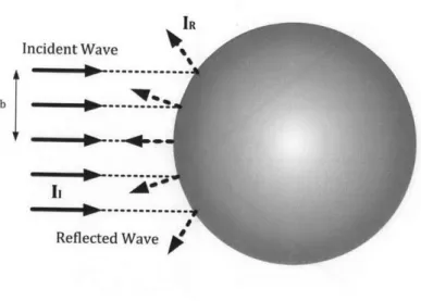
IR
Incident Wave %
b ----
...-A Reflected Wave
Figure 2-2: Specular scattering of a planar incident wave on a spherical object
Figure 2-2 illustrates the specular scattering at a spherical object with a plane
incident wave. Assuming the cross-section of the incident beam is a circle with the radius of b, the intensity ratio of a reflected wave (IR) to a incident wave (I,) is given
as [14]:
IR(r) wrb2
~r rr2 RF|2
(2.12)
I, 47rr2
where r is approximately the distance from the object. The intensity of the reflected wave is inversely proportional to r2
and directly proportional to JRF 2.
Diffusive Scattering
In biological tissue, micro structures and scattering objects whose sizes are in sub-wavelength scale also cause scattering in a different mechanism, called diffusive scattering. Provided that the wavelength of diagnostic ultrasound ranges from 150 to 770 pm for an operating frequency from 2 to 10 MHz, most of scattering falls into
the diffusive scattering. Contrary to the specular scattering, the diffusive scattering
occurs when the roughness of the boundary is much smaller than the wavelength of an incident wave. While the specular scattering helps visualize distinct boundaries between different tissues, the diffusive scattering allows to display different patterns produced from different tissue structures. Therefore, tissue is often modeled as a set of small scatterers, defined as objects to cause scattering, of a sub-wavelength
scale. In addition, the diffusive scattering caused by erythrocytes (i.e., red blood cells) essentially enables Doppler ultrasound to estimate a blood flow velocity. The erythrocyte is a biconcave disc of a 7 pim diameter and a 2 prm thickness, and blood consists of 45% of the erythrocyte for healthy men and 42% for women in a volume ratio, known as hematocrit. Since the erythrocytes account for 98% of particles in blood, the scattering from blood is mainly attributed to the erythrocytes [15].
Ki, Pi Is Incident Wave 00 E Scattered Wave
Figure 2-3: Diffusive scattering of a planar incident wave on a spherical object
The diffusive scattering is well analyzed as a Rayleigh scattering. Rayleigh scat-tering leads to the expression of the intensity of a scattered wave (Is) from a sub-wavelength spherical object, and its expression is given by [14]
Is(r) _ 167r4a6 3(1 - p2/PI) cos 0 + 2
Ii 9A4r2 1 + 2
P2/P1 ( 2
where a is the radius of the object, pi is the density and ri is the compressibility in Figure 2-3. In the Rayleigh scattering, the intensity of the scattered acoustic wave depends on the fourth power of the wavelength and the sixth power of the size of the object.
parame-Scattering Volume
Incident Wave Scattered Wave
Solid angle for - dfl receving
- scattered wave
Figure 2-4: Diffusive Scattering of an incident wave on scattering volume from [18]
ters defined from a scattering volume containing numerous scatterers are realistic in describing the acoustic properties of tissue as shown in Figure 2-4. For individual scatterer, a differential scattering cross-section (cds) is defined as the ratio of power
scattered in particular direction (P) to the incident intensity (I) per unit solid angle (Q), and the cross-section is expressed as following.
(1 d PS(07#
O's(, #) = 1 (2.14)
dQ I
If the incident wave is scattered from the randomly distributed scatterers, the scat-tered power is proportional to the number of scatterers. Therefore, a differential scattering coefficient (Pu) can be expressed as
Pds (0, #) = nZsiOdsi(O,) (2.15)
where Odsi and nsi are the differential scattering cross-section and the number density distribution of individual scatterer types. Particularly, the scattered intensity directly returning to a source such as an ultrasonic transducer is of great importance, and the differential scattering coefficient in this case is denoted as a backscattering coefficient
Pbs = pds 7r, 0). A scattering coefficient, then, is defined as the total power scattered in space per unit intensity and per unit scattering volume, and it is given as:
Ps = Js(10, #)dQ (2.16)
The backscattering coefficient of blood sample with hematocrit of 26 at 5 MHz is
reported around 2 * 10- 3/n - sr [19].
Table 2.2: Relative magnitude of scattered acoustic wave in biological tissues from [16]
Tissue Signal Level (dB)
Fat/muscle (reference*) 0
Placenta -20
Liver -30
Kidney -40
Blood -60
*reference level taken from typical organ boundary
Diffractive Scattering
For the scatterer and boundary whose roughness is similar to the wavelength, diffractive scattering occurs. In the diffractive scattering, the scattered wave is con-sidered to originate from scatterer surface which acts as a secondary source [14]. The differential scattering cross-section of a spherical object is written as
(2.17) US(O) -(-y,+- 2vcosO)(sin(k~a) - ak, cos(ksa))1
-k
___ fP
where k = -, k8 = 2k sin(O), K= K" and 7,. = P -", and
f
denotes the smallfluctuations from the host material (a). In the diffractive scattering, a scattering pattern shows complicated dependency on a scattering angle (0), the radius of the scatterer (a) and the wavelength (A).
2.2
Ultrasonic Transducer Characterization
2.2.1
Piezoelectric Element Physics
An ultrasonic transducer employs a piezoelectric material which converts an elec-trical signal to a mechanical force and vice versa [18]. For example, lead zirconate titanate (PZT) is commonly used as the piezoelectric material of modern transducer elements. Ceramics and quartz, which are not naturally piezoelectric, are made piezo-electric during their production by placing them into a high piezo-electric field at very high temperature [17]. The transducer generates an acoustic wave when excited with an alternating voltage, and the frequency of the transmitted acoustic wave is same as the frequency of the voltage signal. Typically, the frequency of the voltage signal matches to a resonant frequency, which is discussed in the following section, of the piezoelectric element. L
b
BackingALoad
Layer - MediumS
S
Bottom Top Electrode ElectrodeFigure 2-5: Piezoelectric element with parallel electrodes
Figure 2-5 shows a basic piezoelectric element schematic consisting of two elec-trodes with the cross-sectional area (A), the thickness (d). When a voltage impulse
excites the element through the electrodes, electric charges accumulate in the region near the top and bottom electrode, thus generating stress. This stress is propagated
as the acoustic wave across the element. Assuming that the electrodes are thin,
and external media have same acoustic impedances, the stress measured at the top electrode shows an impulse followed by a subsequent stress impulse induced at the bottom electrode after a propagation delay, and the stress and its frequency response
are expressed as [20]: S(t) hC (6(t) - 6(t - ) (2.18a) 2A c hC0
wrf
IS(f), = A sin( ) (2.18b) A 2 fowhere Co is the clamped (zero-stress) capacitance, h is the piezoelectric constant, and
c is the speed of sound in the piezoelectric element. The frequency response shows
resonant frequencies at the odd multiples of a fundamental frequency at fo = '. The thickness of the element mainly determines the fundamental resonant frequency.
The piezoelectric element is generally regarded as an acoustic resonator including cases when reflection exists due to acoustic impedance mismatch. However, three dimensional nature of the element unavoidably generates multiple resonant modes. For most of the piezoelectric elements, the thickness (d) is far smaller than the width
(L) and height (b) of the element. Therefore, other resonant modes are usually
negligible [18].
In diagnostic ultrasonography, finer axial resolution (i.e., imaging resolution on a beam axis) is often desirable to identify minuscule tissue structures. A spatial pulse length, determined by both the time duration of the applied voltage pulse and the impulse response of the ultrasonic transducer, sets the axial resolution of imaging systems. In order to achieve a short impulse response, a damping material is usually placed in a backing layer at the cost of reduced efficiency of the transducer. The quality factor (Q-factor) is defined as the reciprocal of the fractional bandwidth of the pulse. For short pulses, the Q-factor is approximately coincides with the number of cycles in the pulse, and the insertion of the damping material lowers the Q-factor at the same voltage excitation, achieving the finer axial resolution [17].
Unlike the previous assumption, the acoustic impedances of the piezoelectric ma-terials differ significantly from load medium (e.g., water, tissue). As a consequence, only fractional acoustic power is transmitted to the load medium. In order to reduce the reflection of the acoustic wave during both a transmit and a receive, a series of matching layers which have intermediate acoustic impedances is inserted to enhance overall acoustic coupling. The optimal thickness of this matching layer is a quarter wavelength [17].
2.2.2 Equivalent Circuit Model
d/2 d/2 --- Acoustic ---2 S Z , Z Zuin \\ZRin *I W Backward Forward - Electrical ---CO C'
3 V
Figure 2-6: KLM equivalent circuit model for a piezoelectric element
To the first order, the piezoelectric element is modeled into an equivalent electri-cal circuit. Mason model [21] utilizes an analogy between acoustielectri-cal parameters (e.g., stress (S) or force and a particle velocity) and electrical parameters (e.g., a voltage and a current) to derive several models for different piezoelectric transducer geome-tries [14]. A KLM model, introduced by Krimholtz, Leedom, and Matthaei [22], is especially useful when only one dominant resonant mode exists, which is a thickness-expander mode in medical ultrasound transducers. The advantage of the KLM model is to separate the acoustic and electrical parts of transduction process through a trans-former shown in Figure 2-6. In addition, the KLM model is especially useful for a
broadband transducer design
[231.
The KLM model shown in Figure 2-6 consists of two acoustic ports and one electric port. The port one leads to the matching layer and the load medium where the acoustic wave propagates. The port two reaches the backing layer. In the KLM model, an artificial acoustic center is created for convenience of analysis even though the stress of the piezoelectric material is induced at the boundaries of the element [18]. In the acoustic domain, an acoustic transmission line accounts for the propagation and resonant behavior of the piezoelectric element. The acoustic transmission line is characterized by the thickness (d), the speed of sound in piezoelectric material (c), and the acoustic impedance (Z). The electrical signal is transformed into the acoustic domain through the transformer with the turns ratio of 1 : $. The electrical domain of
the KLM model consists of the clamped capacitance (CO) and a negative
capacitance-like component (C') which models an acoustoelectric feedback. The turns ratio (p)
and C' is expressed as [14]
#=kT( )I sinc( )(2.19)
woCoZc 2wo
C = CO (2.20)
ksinc( )
where kT is an electromechnical coupling constant. The electrical input impedance of a loaded transducer provides insight into a driver and receiver design. For simplicity of analysis, only the port one is loaded. Then, the electrical input impedance from port three is given as [23]
1 1
ZT (w) + Za= + Ra + jXa (2.21a)
jwCo jiwCo Ra = k (WO) 2(1 - cos(WW))2 (2.21b) wwoCo w wo 2k 2 1 7FW g Xa = ( sin -(1- - cos(
))
(2.21c) FwOCO W WO 2 wothat the complex acoustic radiation impedance becomes purely real at the resonant frequency. However, due to non-ideality, a matching network (such as a series in-ductor) at the electrical port may be inserted to compensate for a capacitive input impedance to minimize power loss from the large capacitive load.
2.2.3
Pressure Field in Continuous Wave
The acoustic wave induced from the piezoelectric element propagates through the load medium from the surface of an ultrasonic transducer. The acoustic wave radi-ating from a finite aperture is considered equivalently as many infinitesimal sources on the aperture radiating spherical waves according to the Huygens' principle [14]. Hence, many spherical waves interfere with each other in both constructively and destructively, and this phenomenon results in a specific pattern, known as a diffrac-tion pattern. Especially, the diffracdiffrac-tion pattern becomes distinct as the dimension of the aperture reaches the wavelength of the radiating wave. In fact, the aperture size of medical ultrasonic transducers (few mm scale) is close to the wavelength of the medical ultrasound (hundreds of pm). Therefore, diffraction explains the detailed acoustic beam pattern in medical ultrasound.
A pressure field amplitude in Figure 2-7 is written in terms of a spatial integral
over the transducer surface to add contributions from each of point sources as [14]
j pockvo e 4wt-k(f-ro)]
r t) PW 0 jp- ) A(iFo)dS (2.22)
27 ' r -ro|
where po is the density of the medium, voA(r-3) is the velocity normal to the surface,
c is the speed of sound and k is the wavenumber. Equation 2.22 is also called the
Rayleigh-Sommerfeld integral [14]. In the region where I--"I I"--"
<
< 1, F -Ir- isexpanded by applying a parabolic approximation (Fresnel approximation) as:
y
x
r R
Figure 2-7: Geometric representation of a transducer aperture and its coordinates
Plugging Equation 2.23 into Equation 2.22 results in:
, j pockvo iIwt-kz)-ik(X2+y2)/2z f ik(x2+y2 )/2zA(x , yo)]eik(xxo±YYO)/zdxdy
) 2Tz fs C
(2.24) Equation 2.24 shows that the beam pattern at the fixed depth (z) is the spatial Fourier transform of e-ik(x±+y2)/2zA(xo, yo). This diffraction pattern is defined as the
Fresnel diffraction. As z > x2 + y2, then the Fresnel diffraction pattern is further
approximated into the Fraunhofer diffraction which states that the beam pattern at the fixed depth is just the spatial Fourier transform of the aperture itself.
Equation 2.24 can be applied to an arbitrary aperture, and analytic solutions for simple geometries (e.g., rectangular or circular) are already presented. Especially, many single element transducers have the circular aperture, and the pressure field in the Fraunhofer region (far-field) of the circular aperture is given as [14]:
jpo-ra2 2J
1(27rRa/Az) (2.25)
where J is the first order Bessel function, and a is the radius of the circular aper-ture. A beam width is defined as a distance between two points where the pressure amplitude drops to a half of maximum. The FWHM (Full Width Half Maximum) beam width is expressed as:
Az
FWHM = 0.7047- (2.26)
a The pressure amplitude on a z-axis is expressed as:
kz
p(O, z, A)I = 2po sin[ ( 1 + (a/z)2 - 1)] (2.27) 2
and a near-to-far field transition depth (z,), also known as the natural focus, occurs at:
a2
Zr = (2.28)
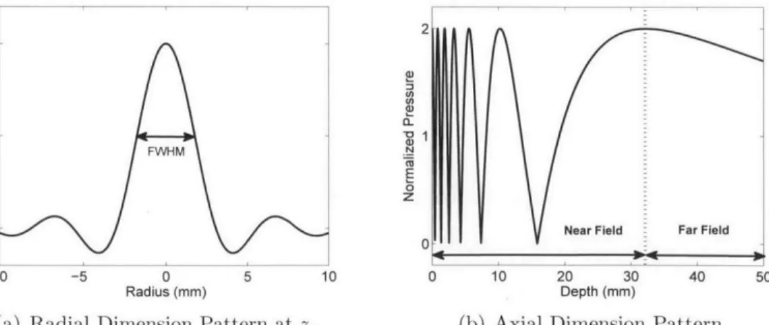
Equation 2.28 shows the natural focus is only relevant to the aperture radius (a) and the wavelength of the acoustic wave (A). Figure 2-8 presents continuous pressure fields in both a radial and an axial dimension. Most of the acoustic energy is concentrated within the beam width. In the axial dimension, the pressure amplitude shows many notches in a near-field while the pressure amplitude monotonically decreases in the
2 U) (n 0.5-FWHM N 0 0 z Z
0 Near Field Far Field
0
-10 -5 0 5 10 0 10 20 30 40 50
Radius (mm) Depth (mm)
(a) Radial Dimension Pattern at zr (b) Axial Dimension Pattern
Figure 2-8: Simulated continuous pressure in a radial axial dimension for a circular aperture of 5 mm radius at continuous 2 MHz ultrasound
MEM
0 0I
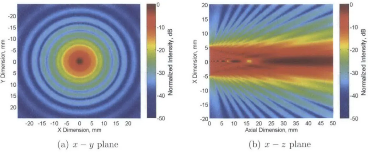
-15 -10 -10 -520 -20 0 0 110 100 -40 -40 2 20 -50 -1520 -50 -20 -15 -10 -5 0 5 10 15 20 0 5 10 15 20 25 30 35 40 45 50 -50X Dimension, mm Axial Dimension, mm
(a) x - y plane (b) x - z plane
Figure 2-9: Simulated continuous pressure a temporal-averaged intensity field in x - z
and x - y plane for a circular aperture of 5 mm radius at 2 MHz ultrasound
far field. Figure 2-9 shows the continuous pressure field amplitude in x - z and x - y plane.
In ultrasonic imaging systems, the beam width determines the lateral resolution of images, thereby requiring a higher operation frequency and a larger aperture for finer lateral resolution. In addition, modern medical ultrasound utilizes a phased array transducer in order to enhance focusing capability, adjust a focal depth and achieve beam steerability. Since the natural focus is the point where significant constructive interference occurs at last, the focal depth adjustment is only achieved within the near-field region.
2.2.4
Pressure Field in Pulsed Wave
Most of medical ultrasonography is operated in a pulsed manner because the pulsed operation eliminates the ambiguity of depth information. Therefore, an operator can target and obtain physiological information at the specific region of interest. Although the analysis of the continuous pressure field provides a great insight on the diffraction
beam pattern, the analysis does not include the exact temporal behavior of a pulsed pressure field. This section briefly describes two powerful techniques for a pulsed pressure field analysis.
From the more general Rayleigh integral, a pressure field description for both continuous and pulsed wave is given based on Huygens' principle again as [15]:
PO Ov(rO7,t - Ir)/ &t
2is , =dS
21T |r- Iroi
=pov(t) * 2 _j _(t- ) dS (2.29)
Ot s 7 r'r -- rO| povn(t) * ht
where h(i?, t) is defined as a spatial impulse response [15]. Equation 2.29 allows to obtain a time domain pressure waveform in space if the spatial impulse response is known. Since the geometry of the aperture determines the spatial impulse response, Equation 2.29 is easily utilized to depict the pressure field waveform for any acoustic waves [15]. The other powerful technique is based on the reciprocity theorem of acoustics, which states a transmitter and a receiver are interchangeable [15]. The implication of the reciprocity theorem is the spatial impulse response is reconstructed by observing the transducer's response to a point source in space radiating a spherical wave. Then, the pulsed pressure field can be obtained similarly using the spatial impulse response as given by Equation 2.29. Figure 2-10 shows the pulsed pressure field amplitude in a x - z and a x - y plane. The pressure field patterns of the continuous (Figure 2-9) and pulsed (Figure 2-10) wave show similarity while the pulsed beam pattern is much smoother in space. Though Equation 2.26 and 2.28 are useful, an acoustic simulator, such as Field II, provides the exact beamwidth and the natural focus of a given aperture in the pulsed ultrasound.
Finally, a received pressure response (pr) is expressed in terms of a spatial
inho-mogeneity (fM) and a pulse-echo impulse response (vpe), including both a transducer
excitation and an electromechanical impulse response, written as [15]:
Pr(, t) = Vpe(t) *t
f
m(r) *r hpe(, t) (2.30)re-spectively. Additionally, h,(r', t) accounts for the spatial impulse response for both transmit and receive.
E E 0 E -20 -15 -10 -5 0 5 10 15 20 X Dimension, mm (a) x - y plane 0 -10 -20 -30 . 0 -40 Z -50 E E 0 E -151 -20 0 5 10 15 20 25 30 35 40 45 50 Axial Dimension, mm (b) x - z plane
Figure 2-10: Simulated pulsed pressure a temporal-averaged intensity field in x - z
and x - y plane for a circular aperture of 5 mm radius at 3 cycles of 2 MHz ultrasound
0 -10 -20 -30 ~0 -40 Z -50
Chapter 3
Hemodynamics of Arterial System
The circulatory system provides various organs and tissues with oxygen and nutrition which are essential to metabolism, and the system disposes carbon dioxide and wastes as well. Especially, arterial blood delivers oxygen and nutrition, and its flow is driven
by arterial blood pressure (ABP) exerted by the contraction of the left ventricle.
Although this simplistic view explains the main role of the heart in the circulatory system, the relationship between the blood flow and the pressure is very complicated and also highly dependent on the mechanics of vascular structures. This chapter begins to focuses on the basic hemodynamics of the arterial system. Thereafter, it introduces the anatomical background of the arterial system.
3.1
Blood Flow Physics
This section introduces basic flow physics assuming a blood vessel is modeled as a cylindrical tube. It begins with the analysis of constant flow followed by pulsatile flow. Typically, the comprehensive description of flow dynamics requires the solution of the Navier-Stokes equation [15], but this section mainly stays within a simple view to provide the clear idea of blood flow physics.
3.1.1
Steady Flow
First of all, fluid is assumed incompressible in macro-scale although the existence of a longitudinal acoustic wave in the fluid acknowledges localized compression. This incompressibility implies a constant volumetric flow rate
(Q)
along an entire rigid tube as given by [15]:Q = Av) = Ai = A2 7T2 (3.1)
where V is the average flow velocity over the cross-section of the tube.
In addition, the mechanical energy (kinetic, potential and internal energy) of the fluid must be conserved, and the description of energy conservation is represented in Bernoulli's equation as [15]:
Pi + 1 +ghi+U1= gh± P2 V2
+ +A2+ U2 (3.2)
Pi 2 P2 2
where g is gravitational acceleration, p is the pressure, p is the density, v is the flow velocity, and U is denoted as internal energy per unit mass. In the human body, blood's density and temperature are almost constant, so its internal energy change is negligible. Therefore, Equation 3.2 somewhat relates the flow velocity and the pressure measured at different height representing different arterial sites.
Another important property of fluid is viscosity originated from shear stress be-tween layers of fluid each of which moves at different velocity. The viscosity (P) is defined as the proportionality between the sheer stress and strain as Equation 3.3a and more generally Equation 3.3b:
dF dv =dA (3.3a) d A dy dv dtt SXy = P( + d) (3.3b) dy dx
where Sxy is the sheer stress, and v, u are the velocities in x and y direction, re-spectively. Figure 3-1 shows the sheer stress between the fluid layers of the different flow velocities. For ideal fluid, called Newtonian fluid, the viscosity is independent of
AF V+AV
AA V
X,v
Figure 3-1: Illustration of force on small fluid volume in a rigid tube from [15]
sheer stress. However, blood is a complex fluid which is described as the suspension of blood cells and plasnia, and the viscosity of the blood changes with the sheer stress. The viscosity of the blood is also dependent on teniperature and hematocrit. Still, given that the hematocrit of human is well controlled between 42-45%, and the body temperature is well regulated to 36.5'C, the viscosity of the blood is often assumed
to be 4 x 10⁻³ kg/m - s [151.
Because of the viscosity of the fluid and the friction from the tube's wall, a velocity profile develops to balance the sheer stress with a driving force. In constant laiinar flow (i.e., fluids flowing in parallel), the velocity profile eventually becomes parabolic and its profile is expressed as:
v(r) Vmax(1 (3.4)
where r is the radius from the axis, Vnax is the maximum velocity, and R is the inner radius of the tube [15]. When the velocity profile becomes parabolic, a viscous drag force at every laminae is balanced against the driving force originated from a pressure gradient, thus maintaining a constant flow velocity at every laminae. The parabolic profile usually develops after the fluid passes through a long rigid tube.
In the vascular system, the blood vessels often branch into smaller vessels, and the velocity profile at the entrance of small branches shows a transient profile other than the parabolic profile. When the branching vessel is significantly smaller, the velocity profile at the entrance is almost flat, known as a plug profile. The velocity

![Figure 2-4: Diffusive Scattering of an incident wave on scattering volume from [18]](https://thumb-eu.123doks.com/thumbv2/123doknet/14470451.522240/28.918.286.661.106.400/figure-diffusive-scattering-incident-wave-scattering-volume.webp)
![Table 2.2: Relative magnitude of scattered acoustic wave in biological tissues from [16]](https://thumb-eu.123doks.com/thumbv2/123doknet/14470451.522240/29.918.204.683.381.564/table-relative-magnitude-scattered-acoustic-wave-biological-tissues.webp)

![Figure 3-6: Illustration of vascular structures in the neck from [29]](https://thumb-eu.123doks.com/thumbv2/123doknet/14470451.522240/53.918.197.699.112.489/figure-illustration-vascular-structures-neck.webp)


