Modelling honeybee visual guidance in a 3-D environment

(1)

HAL Id: hal-02010550

https://hal-amu.archives-ouvertes.fr/hal-02010550

Submitted on 7 Feb 2019

HAL is a multi-disciplinary open access

archive for the deposit and dissemination of sci-entific research documents, whether they are pub-lished or not. The documents may come from teaching and research institutions in France or

L’archive ouverte pluridisciplinaire HAL, est destinée au dépôt et à la diffusion de documents scientifiques de niveau recherche, publiés ou non, émanant des établissements d’enseignement et de recherche français ou étrangers, des laboratoires

Modelling honeybee visual guidance in a 3-D

environment

G. Portelli, Julien Serres, F. Ruﬀier, N. Franceschini

To cite this version:

G. Portelli, Julien Serres, F. Ruﬀier, N. Franceschini. Modelling honeybee visual guidance in a 3-D environment. Journal of Physiology - Paris, Elsevier, 2010, 104 (1-2), pp.27-39. �10.1016/j.jphysparis.2009.11.011�. �hal-02010550�

(2)

Modelling honeybee visual guidance in a 3-D

environment

Portelli G., Serres J., Ruffier F., and Franceschini N.

The Institute of Movement Sciences, UMR6233 CNRS - Aix-Marseille Uni., CP938, 163 ave. Luminy, 13288 Marseille Cedex 09, France

Abstract

In view of the behavioral findings published on bees during the last two decades, it was proposed to decipher the principles underlying bees’ autopi-lot system, focusing in particular on these insects’ use of the optic flow (OF). Based on computer-simulated experiments, we developed a vision-based au-topilot that enables a “simulated bee” to travel along a tunnel, controlling both its speed and its clearance from the right wall, left wall, ground, and roof. The flying agent thus equipped enjoys three translational degrees of freedom on the surge (x), sway (y), and heave (z) axes, which are uncoupled. This visuo-motor control system, which is called ALIS (AutopiLot using an Insect based vision System), is a dual OF regulator consisting of two inter-dependent feedback loops, each of which has its own OF set-point. The experiments presented here showed that the simulated bee was able to navi-gate safely along a straight or tapered tunnel and to react appropriately to any untoward OF perturbations, such as those resulting from the occasional lack of texture on one wall or the tapering of the tunnel. The minimalistic visual system used here (involving only eight pixels) suffices to jointly con-trol both the clearance from the four walls and the forward speed without

(3)

having to measure any speeds or distances. The OF sensors and the simple visuo-motor control system we have developed account well for the results of ethological studies performed on honeybees flying freely along straight and tapered corridors.

Key words: Optic Flow (OF), computational neurosciences, honeybee, speed control, biomimetics, obstacle avoidance.

(4)

1. INTRODUCTION 1

Winged insects are able to navigate in unfamiliar environments, using the 2

optic flow (OF) (Gibson, 1950) generated by their own motion (Horridge, 3

1987). Insects make use of the OF to avoid lateral obstacles (Srinivasan et 4

al., 1991; Serres et al., 2008b), control their speed (Preiss, 1987; Baird et al., 5

2005, 2006) and height (Baird et al., 2006; Franceschini et al., 2007), cruise 6

and land (Srinivasan et al., 1996, 2000; Franceschini et al., 2007). Behavioral 7

studies on flying insects have inspired several researchers to develop visually 8

guided mobile robots (Pichon et al., 1989; Franceschini et al., 1992; Coombs 9

and Roberts, 1992; Duchon and Warren, 1994; Santos-Victor et al., 1995; 10

Weber et al., 1997; Lewis, 1997; Netter and Franceschini, 2002; Ruffier and 11

Franceschini, 2003; Humbert et al., 2007; Beyeler et al., 2007). 12

The LORA III autopilot we previously developed was based on a pair of 13

lateral OF regulators steering a fully actuated hovercraft, in which the surge 14

and sway dynamics were uncoupled (Serres et al., 2008a). The LORA III 15

autopilot was found to account for the behaviors such as centering and speed 16

control observed in bees flying along stationary and nonstationary corridors 17

(Srinivasan et al., 1991) as well as tapered corridors (Srinivasan et al., 1996). 18

LORA III also accounted for the novel findings on wall-following (Serres et 19

al., 2008b), which the previous hypothesis (“optic flow balance” hypothesis) 20

could not explain. 21

In the ALIS autopilot described here, the LORA III autopilot principle 22

is extended to include the vertical plane. The problem consisted here of de-23

veloping a functional scheme for a joint speed control and obstacle avoidance 24

system that would take not only lateral obstacles but also ventral obstacles 25

(5)

(Baird et al., 2006; Franceschini et al., 2007), and dorsal obstacles (Vickers 26

and Baker, 1994) into account. The ALIS autopilot we designed was used 27

to test a simulated honeybee, in which all the translational degrees of free-28

dom (DOF) (surge, sway, and heave) were uncoupled (Ellington, 1984). In 29

our simulations, the flying agent was endowed with the following novel flight 30

features: 31

• use of 2-D model for photoreceptor sensitivity, 32

• use of the walls, ground, and roof, which were all textured with natural 33

scenes, 34

• use of a new linearized model for flying bees’ locomotion. 35

• use of an optic flow regulator based on both the lateral and the vertical 36

OFs. 37

The ALIS autopilot regulates the OF thanks to the positioning and for-38

ward control systems with which it is equipped, according to the following 39

principles: 40

(i) the first OF regulator adjusts the bee’s forward speed so as to keep 41

whichever sum of the two opposite OFs (i.e., left/right or ventral/dorsal) is 42

maximum equal to a forward OF set-point. The outcome is that the bee’s 43

forward speed becomes proportional to the smallest dimension (either the 44

width or the height) of the flight tunnel. The forward speed attained will be 45

such that the OF generated equals the value of the forward OF set-point. 46

(ii) the second OF regulator adjusts the bee’s lateral or vertical position 47

so as to keep whichever OF is maximum (among the four OFs : left, right, 48

(6)

ventral, and dorsal) equal to the positioning OF set-point. The outcome is 49

that the clearance from the nearest tunnel surface (the walls, ground, or roof) 50

becomes proportional to the bee’s current forward speed, as defined in (i). 51

The clearance from the nearest tunnel will be such that the OF generated 52

equals to the positioning OF set-point. 53

The ALIS autopilot enables the agent to perform obstacle avoidance by 54

performing maneuvers involving only translational DOFs, unlike the obsta-55

cle avoidance schemes based on body saccades that involve rotational DOFs 56

(Lewis, 1997; Schilstra and van Hateren, 1999; Tammero and Dickinson, 2002; 57

Beyeler et al., 2007). The ALIS autopilot operates without relying on any 58

speed or distance measurements. It also differs fundamentally from previ-59

ous “insect-like” navigation systems based on speed or distance regulation 60

(Dickson et al., 2006). 61

In section 2, the dynamical model for the simulated bee is described in 62

terms of its three translational DOFs. In section 3, the simulation set-up 63

used to test the ALIS autopilot on board the simulated bee is described. 64

Section 4 describes the ALIS autopilot in detail. Section 5 gives the results 65

of computer-simulated experiments carried out on the simulated bee, which 66

is able to perform various tasks such as takeoff, straight and tapered tunnel-67

following, and to react appropriately to any local lack of lateral or dorsal 68

OF. 69

2. DYNAMICAL MODEL FOR BEES’ FLIGHT 70

Here we focus on the visuomotor feedback loops that may explain how 71

a flying insect controls its speed and avoids obstacles. A linearized model 72

(7)

for the bee’s dynamics is proposed in terms of the three translational DOFs 73

(surge, sway, and heave dynamics). Linearization was justified here by the 74

limited range of speeds (0-2 m/sec) possible. The value of the three rota-75

tional DOFs was kept at zero because bees are known to fly straight to their 76

nectar source (von Frisch, 1948; Riley et al., 2003). In our experiments, the 77

simulated insect was not subjected to any wind disturbances: the ground-78

speed was therefore taken to be equal to the airspeed. The bee’s dynamic 79

performances in the three translational DOFs will be described in detail be-80

low. 81

(FIGURE 1 about here) 82

2.1. Bees’ Surge dynamics 83

Experiments on fruitflies (David, 1978) and honeybees (Nachtigall et al., 84

1971; Esch et al., 1975) have shown that flying insects gain forward speed 85

by pitching their mean flight-force vector ~F forward at a small angle θpitch

86

(≤ 20 deg) with respect to the vertical (Fig. 1A, B). By slightly changing the 87

wing stroke plane pitch angle θpitch, the insect generates a forward Thrust T ,

88

which hardly affects the vertical Lift L (Ellington, 1984). In bees, the mean 89

flight-force vector orientation differs from the body orientation, forming a 90

fixed angle (Nachtigall et al., 1971; Ellington, 1984). 91

2.2. Bees’ Sway dynamics 92

In flying hymenopterans, sideslip motion results from roll changes (Elling-93

ton, 1984; Zeil et al., 2008). The wing stroke plane roll angle θroll therefore

94

drives the Sideways thrust S (Fig. 1A, C). 95

(8)

2.3. Bees’ Heave dynamics 96

The mean flight-force vector ~F (Eq. 1)resulting from the wing stroke am-97

plitude Φ (Dillon and Dudley, 2004; Altshuler et al., 2005) can be expressed 98

in terms of forward Thrust T , Side thrust S, and vertical Lift L. 99 ~ F =          T S L          =         

F (Φ) · sin θpitch· cos θroll

F (Φ) · cos θpitch· sin θroll

F (Φ) · cos θpitch· cos θroll

         (1)

where F (Φ) is the force generated by an amplitude Φ of the wing stroke. 100

At small angles (θpitch and θroll) angles, L is roughly equal to F . The wing

101

stroke amplitude Φ therefore mainly drives the vertical lift L. 102

2.4. Calculating the gain between the wing stroke amplitude and the lift 103

The lift produced by a bee depends on both the density ρ of the air and 104

the wing stroke amplitude Φ (Dudley, 1995). In order to determine the gain 105

Kwingbetween the wing stroke amplitude Φ and the lift L, we used the results

106

of experiments on hovering bees that were carried out in media with different 107

densities. Hovering bees were filmed in normal air (ρAir = 1, 21 kg/m3) and

108

in heliox (ρHeliox = 0, 41 kg/m3) (Altshuler et al., 2005). In the low density

109

heliox, bees were found to increase their wing stroke amplitude Φ from 90 deg 110

to 130 deg, while keeping their wingbeat frequency constant. In these two 111

hovering situations (θpitch = θroll = 0◦), the lift L is equal to the weight:

112

LHeliox(Φ = 130 deg) = LAir(Φ = 90 deg) = m · g ∼= 1 mN

In a steady state analysis, the lift is proportional to the density at a given 113

stroke amplitude Φ = 130 deg (Ellington, 1984; Sane and Dickinson, 2002): 114

(9)

LAir(Φ = 130 deg)/ρAir = LHeliox(Φ = 130 deg)/ρHeliox

We therefore calculated LAir(Φ = 130 deg) ∼= 3 mN, and obtained the

115

mean sensitivity of the lift production to the wing stroke amplitude, Kwing=

116

∂LAir/∂Φ = 50 µN/deg in hovering bees (ΦHover = 90 deg).

117

2.5. The Linearized Flying Bee model 118

At small pitch levels | θpitch |≤ 20 deg and roll | θroll |≤ 20 deg angles, each

119

component of the mean flight-force vector ~F can be linearized on the surge, 120

sway, and heave axes (Eq. 2) as a function of the pitch angle θpitch, the roll

121

angle θroll, and the wing stroke amplitude Φ = ΦHover+ ∆Φ, respectively:

122 ~ F =          T S L          =          m · g · θpitch m · g · θroll Kwing· (ΦHover+ ∆Φ)

with Kwing·ΦHover=m·g (2)

The following linearized system of equations was referred to the bee’s 123

center of gravity as follows: 124

m · d~V /dt + Z · ~V = ~F + m · ~g (3)

where ~V is the mean speed vector, ~F is the mean flight force vector, ~g is 125

the gravity constant, m = 100 mg (the bee’s mass), and Z is the translational 126

viscous friction matrix Z =      ζ 0 0 0 ζ 0 0 0 ζ      . 127

(10)

The time constant along a translational DOF can be defined by the ratio 128

between the mass and the translational viscous friction coefficient. To the 129

best of our knowledge, no data are available so far on the sway and heave time 130

constants in the case of freely flying honeybees but these values are likely to 131

be of the same order as the surge time constant. The bee’s surge time constant 132

τ = m/ζ = 0.22 sec can be estimated from bees’ landing data (Srinivasan 133

et al., 2000) and from bees OF based autopilot system (Franceschini et al., 134

2007). In what follows, bee sway and bee heave time constants are assumed 135

to be equal to the bee surge time constant. 136

Equation 3 can be written as follows: 137          τ · dVx/dt + Vx = (m · g)/ζ · θpitch τ · dVy/dt + Vy = (m · g)/ζ · θroll τ · dVz/dt + Vz = (Kwing/ζ) · ∆Φ (4)

The sensitivity Ksurge of the forward speed Vx to the pitch angle θpitch

138

can be determined from figure 2b in Esch et al. (1975) and estimated as 139

follows: 140

Ksurge=| ∂Vx/∂θpitch|= 0.10 m.sec−1.deg−1

Ksway is assumed to have a similar value: Ksway = Ksurge

141

The Laplace transfer functions giving the bee’s surge dynamics GVx(s), 142

sway dynamics GVy(s) , and heave dynamics GVz(s) can therefore be written 143

as follows: 144

(11)

                 GVx(s) = Vx(s) θpitch(s) = Ksurge 1 + τsurge· s = 0.10 1 + 0.22 · s (5a) GVy(s) = Vy(s) θroll(s) = Ksway 1 + τsway · s = 0.10 1 + 0.22 · s (5b) GVz(s) = Vz(s) ∆Φ(s) = Kwing/ζz 1 + τheave · s = 0.11 1 + 0.22 · s (5c) The pitch angle was limited here to | θpitch |≤ 20 deg so as to keep the

145

maximum forward speed range to Vx M ax = 2 m/sec, and the roll angle was

146

limited to | θroll |≤ 5 deg so as to keep the maximum lateral speed range

147

to Vy M ax = 0.5 m/sec. Bees are thought to reach the maximum stroke

148

amplitude Φmax = 140 deg and the minimum stroke amplitude Φmin =

149

70 deg (Dudley, 2000; Dillon and Dudley, 2004). The maximum ascent speed 150

Vz U pM ax and the maximum descent speed Vz DownM ax on the heave-axis are

151 therefore: 152                Vz U pM ax = (6a)

(Kwing/ζz) · (Φmax− ΦHover) = 5.5 m/sec

Vz DownM ax = (6b)

(Kwing/ζz) · (ΦHover− Φmin) = −2.2 m/sec

The bees’ ascent speed, was calculated from figure 7b in Srinivasan et 153

al. (2000) and found to be equal to ≈ 2 m/sec. The bees’ descent speed 154

measured during landing manoeuvers reaches a value of 2 m/sec (figure 6d 155

in Srinivasan et al. (2000)): this value is quite similar to our own predictions 156

(Eq. 6). In order to limit the vertical speed (| Vz |= 2 m/sec), we set the

157

maximum stroke amplitude at | ∆Φ |≤ 18 deg. 158

(12)

3. SIMULATION SET-UP 159

3.1. Simulated 3-D environment 160

The simulated 3-D visual environment consisted of a straight or tapered 161

flight tunnel (6 meters long, 1 meter wide, and 1 meter high), the four walls 162

of which were lined with high resolution photographs of natural panoramic 163

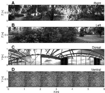
scenes (Brinkworth and O’Carroll, 2007). These images were converted into 164

256 grayscale levels and resized keeping the original size ratios. One image 165

pixel corresponded to one millimeter of the simulated environment (Fig. 2). 166

The four natural grayscale images are shown in Fig. 2: right wall (Fig. 2A), 167

left wall (Fig. 2B), roof (Fig. 2C), and ground (Fig. 2D). 168

3.2. Optic flow generated by the bee’s own motion 170

The simulated bee was assumed to be flying at a speed vector ~V along the 171

flight tunnel covered with natural-scene textures (Fig. 2). It has been shown 172

that hymenopterans stabilize their gaze by compensating for any body rota-173

tions (Zeil et al., 2008), in much the same way as the blowfly does (Schilstra 174

and van Hateren, 1999). The bee’s head orientation was therefore assumed to 175

be locked to the X-axis of the tunnel. Since any rotation is compensated for, 176

each OF sensor will receive a purely translational OF, which is the angular 177

velocity of the environmental features detected by the lateral (diametrically 178

opposed) and vertical (also diametrically opposed) OF sensors (Fig. 3). 179

The translational OF can be defined simply as the forward speed-to-180

distance ratio (expressed in rad/sec) in line with (7). 181

(13)

ωi = Vx/Di, with i ∈

n

Rght, Lef t, V trl, Drslo (7)

where Vx is the bee’s forward speed, DRght, DLef t are the distances to the

182

side (right and left) walls, and DV trl, DDrsl are the distances to the ground

183

(ventral eye) and to the roof (dorsal eye) (Fig. 3). Each OF sensor receives 184

its own OF, which can be a right OF (ωRght), a left OF (ωLef t), a ventral OF

185

(ωV trl), or a dorsal OF (ωDrsl).

186

3.3. OF sensors on board the simulated bee 188

Bees are endowed with two compound eyes, each of which is composed of 189

4500 ommatidia. The visual axes of two adjacent ommatidia are separated 190

by an interommatidial angle ∆ϕ, which varies from one region of the eye to 191

another (Seidl and Kaiser, 1981). Each ommatidium is composed of a lens 192

and nine photoreceptor cells with identical receptive fields. Six of these cells 193

have a green spectral sensitivity (Wakakuwa et al., 2005) and are involved 194

in motion vision. These photoreceptor cells are connected to three succes-195

sive visual optic lobes: the lamina, the medulla, and the lobula. Further 196

down the visual processing chain, descending neurons have been found to re-197

spond to object velocity (Velocity-Tuned motion-sensitive neurons VT cells 198

in Ibbotson (2001)). VT neurons respond monotonically to front-to-back 199

translational movements, and therefore act like real OF sensors. Our sim-200

ulated bee is equipped with only four OF sensors (two lateral, one ventral, 201

and one dorsal sensor, Fig. 3A). Each of these sensors consists of only two 202

photoreceptors (two pixels) driving an Elementary Motion Detector (EMD). 203

(14)

The visual axes of the two photoreceptors are assumed to be separated by an 204

angle ∆ϕ = 4 deg. Each photoreceptor’s angular sensitivity is assumed to be 205

a Gaussoid function with an acceptance angle (angular width at half height) 206

∆ρ = 4 deg, and a total field of view of 10.4 deg × 10.4 deg. The photorecep-207

tors’ output was computed at each time step (0.5 msec) by multiplying two 208

matrixes: 209

• a matrix representing the visible local natural scene (Fig. 2), 210

• a matrix representing the insect-like photoreceptor Gaussoid sensitivity. 211

The “time-of-travel” scheme of the bio-inspired EMD developed by Frances-212

chini’s research group has been previously described in detail (Blanes, 1986; 213

Pudas et al., 2007; Aub´epart and Franceschini, 2007; Franceschini et al., 214

2009). The response of this OF sensor is a monotonic function of the angular 215

velocity within a 10-fold range (from 40 deg/sec to 400 deg/sec) (Ruffier and 216

Franceschini, 2005), resembling that of the Velocity-Tuned motion-sensitive 217

descending neurons found to exist in honeybees(VT neurons: Ibbotson, 2001). 218

4. THE ALIS AUTOPILOT 219

The simulated bee is controlled by an autopilot called ALIS (which stands 220

for AutopiLot using an Insect-based vision System), which is reminiscent of 221

both the OCTAVE autopilot for ground avoidance (Ruffier and Franceschini, 222

2005) and the LORA III autopilot for speed control and lateral obstacle 223

avoidance (Serres et al., 2008a) previously developed at our laboratory. The 224

ALIS autopilot relies, however, on four OF measurements: right, left, ventral, 225

and dorsal. We designed the ALIS autopilot assuming that speed control 226

(15)

and obstacle avoidance problems could be solved in a similar way in both the 227

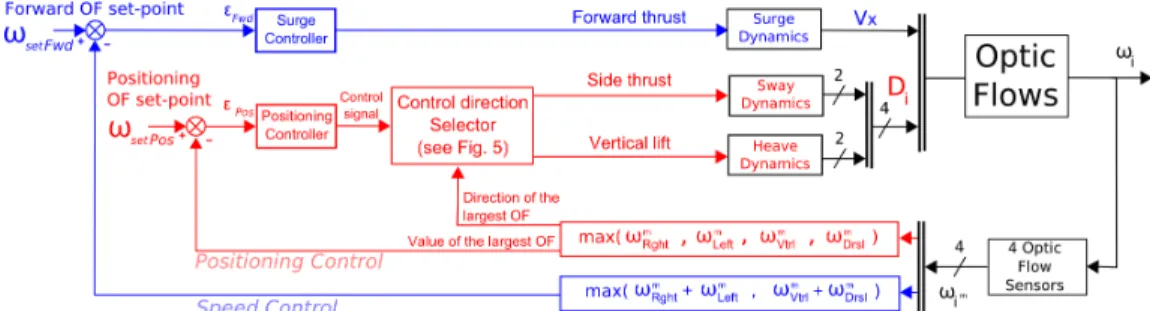
horizontal and vertical planes. The ALIS autopilot consists of two visuomotor 228

feedback loops: the speed control loop (on the surge axis) and the positioning 229

control loop (on the sway and heave axes). These two loops work in parallel 230

and are interdependent. Each of them involves multiple processing stages 231

(Fig. 4), and each has its own OF set-point: the forward OF set-point and 232

the positioning OF set-point, respectively. In this dual control system, neither 233

the speed nor the distance from the tunnel surfaces (walls, ground, or roof) 234

need to be measured. The simulated bee will react to any changes in the OFs 235

by selectively adjusting the three orthogonal components Vx, Vy, and Vz of

236

its speed vector ~V . 237

(FIGURE 4about here) 238

4.1. Forward speed control and forward speed criterion 239

The speed control loop was designed to hold the maximum sum of the two 240

diametrically opposed OFs (measured in the horizontal and vertical planes) 241

constant and equal to a forward OF set-point ωsetF wd. The ALIS autopilot

242

does so by adjusting the forward thrust T (that will determine the forward 243

speed Vx). In other words, this regulation process consists in first determining

244

whether the sum of the OFs measured in the horizontal plane (ωm

Rght+ ωLef tm )

245

or the sum of those measured in the vertical plane (ωm

V trl + ωmDrsl), is the

246

larger of the two. The larger of the two sums is then compared with the 247

forward OF set-point ωsetF wd (blue loop, Fig. 4). The forward OF set-point

248

was set at: ωsetF wd = 4.57 V (i.e., 540 deg/sec). This value was based on that

249

recorded in freely flying bees (Baird et al., 2005). The error signal εF wd (the

250

input to the surge controller) is calculated as follows: 251

(16)

εF wd = ωsetF wd− max[(ωRghtm + ω m Lef t), (ω m V trl+ ω m Drsl)] (8)

The surge controller was tuned using the same procedures as those previ-252

ously described in the case of the LORA III autopilot (Serres et al., 2008a). 253

4.2. Positioning control and positioning criterion 254

The positioning control loop is in charge of positioning the bee with 255

respect to either the side walls or the ground or the roof of the tunnel. 256

Whether this positioning involves motion on the sway or the heave axis 257

depends on whether the maximum OF measured is in the horizontal or 258

vertical plane. The regulation process adopted here is based on the max-259

imum value of the four OFs measured (max(ωm

Rght, ωLef tm , ωmV trl, ωDrslm ), the

260

red loop in Fig. 4), i.e., the value given by the nearest tunnel surface (walls, 261

ground, or roof). This OF regulator is designed to maintain whichever of 262

the four OFs measured is the larger equal to the positioning OF set-point 263

ωsetP os. The larger OF measured is compared with ωsetP os, which was set

264

at: ωsetP os = 2.4 V (i.e., 315 deg/sec). This value was again based on that

265

recorded in freely flying bees (Baird et al., 2005). The error signal εP os (the

266

input to the positioning controller) is calculated as follows: 267 εP os= ωsetP os− max(ωmRght, ω m Lef t, ω m V trl, ω m Drsl) (9)

The positioning controller was tuned using the same procedures as those 268

previously described in the case of the LORA III autopilot (Serres et al., 269

2008a). 270

(FIGURE 5about here) 271

(17)

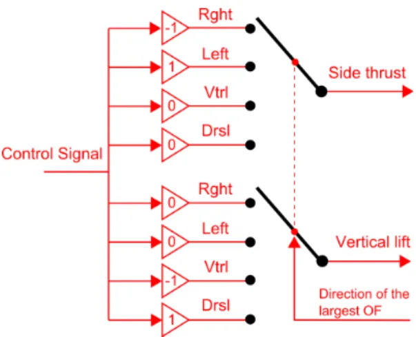
The surface that will be followed (walls, ground or roof) is specified by 272

a Control direction Selector (Fig. 4, 5). The positioning control signal 273

is multiplied by a direction factor that corresponds to the direction of the 274

maximum OF signal. Note that the sway and heave dynamics can be driven 275

alternately, depending on whichever (lateral or vertical) OF is maximum at 276

any given time. The input to the type of dynamics is not commanded is then 277

set at zero (Fig. 5) (Side thrust = 0 or Vertical lift = 0). The simulated 278

bee will react to any unexpected changes in the OFs measured by adjusting 279

either its lateral speed Vy (and hence its lateral position) or its vertical speed

280

Vz (and hence its vertical position). The OF regulator will always react to

281

the nearest of the four tunnel surfaces. 282

5. SIMULATION RESULTS 283

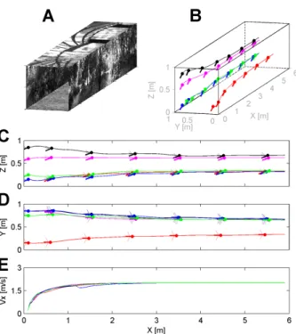
5.1. Automatic tunnel-following 284

In Fig. 6, the simulated environment is a straight tunnel 6 meters long, 285

1 meter wide, and 1 meter high. Fig. 6A shows a perspective view. Walls, 286

ground, and roof were lined with natural grayscale images (Fig. 2). The 287

simulated bee enters the tunnel at the speed Vx0 = 0.2 m/sec and with the

288

initial coordinates x0 = 0.1 m, and various couples of y0 and z0 (Fig. 6B).

289

Fig. 6C shows the five trajectories in the vertical plane (x, z) and Fig. 6D 290

in the horizontal plane (x, y), plotted every 500 msec. Each bar indicates 291

the honeybee’s body orientation, which is known to form a fixed angle with 292

the orientation of the mean flight-force vector (Nachtigall et al., 1971; David, 293

1978). 294

The simulated bee can be seen to have gradually increased both its height 295

(18)

of flight (Fig. 6C) and its right clearance (Fig. 6D) to 0.33 m, while the for-296

ward speed (Fig. 6E) increased automatically up to 2 m/sec (i.e., the maxi-297

mum speed allowed) whichever is the initial positions. 298

These results show that the ALIS autopilot caused the simulated bee to 299

travel safely along the tunnel, while reaching a given forward speed and a 300

given clearance from the walls. 301

(FIGURE 6 and FIGURE 7 about here) 302

5.2. Effect of the local absence of contrast on one of the internal faces of the 303

tunnel 304

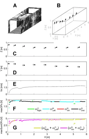
Fig. 7 shows successful tests on the behavior of the simulated bee in the 305

presence of “no contrast” zones on the left wall or the roof of the tunnel. 306

These “no contrast” zones could be either a real aperture or a lack of texture 307

(Fig. 7A). The simulated bee was made to enter the tunnel at speed Vx0 =

308

0.2 m/sec with the initial coordinates x0 = 0.1 m, y0 = 0.85 m, z0 = 0.85 m

309

(Fig. 7B). Fig. 7C shows the trajectory in the vertical plane (x, z) and Fig. 7D 310

in the horizontal plane (x, y), plotted every 500 msec. 311

As can be seen from Fig. 7, the simulated bee was not greatly disturbed 312

by either the 2-meter long aperture encountered on its left-hand side (at the 313

beginning of the tunnel) or a similar aperture entering its dorsal field of view 314

(at the end of the tunnel). 315

The positioning criterion (Fig. 7F) could select either the left or dor-316

sal EMD output (ωm

Lef t or ωDrslm ) when there were no lateral or vertical OF

317

outputs because of the presence of “no contrast” zones (from X= 0.5 m to 318

X= 2.5 m and from X= 3.5 m to X= 5.5 m). The positioning criterion caused 319

(19)

the simulated bee to keep a dorsal clearance DDrsl= 0.35 m (Fig. 7C) and a

320

left clearance DLef t= 0.39 m (Fig. 7D) throughout its journey.

321

The forward criterion (Fig. 7G) could select either the vertical or horizon-322

tal EMD output when there were no lateral or vertical OF outputs because 323

of the “no contrast” zones encountered (from X= 0.5 m to X= 2.5 m and 324

from X= 3.5 m to X= 5.5 m). This criterion caused the simulated bee to 325

maintain a relatively constant speed Vx = 1.85 m/sec throughout its journey

326

(Fig. 7E). 327

These results show that the ALIS autopilot enabled the simulated bee to 328

travel safely along the tunnel without being greatly disturbed by the presence 329

of a lateral or dorsal “no contrast” zone. 330

5.3. Automatic terrain-following 331

Fig. 8 shows successful tests on the behaviour of the simulated bee on a 332

sloping terrain (slope angle 7,deg). As this sloping zone gradually affected 333

the relative distance from the bee to the ground DV trl, it acted like an OF

334

perturbation (Fig. 8A). The simulated bee was made to enter the tunnel 335

at the speed Vx0 = 0.2 m/sec with the initial coordinates x0 = 0.1 m, y0 =

336

0.85 m, z0 = 0.15 m (Fig. 8B). Fig. 8C shows the trajectory in the vertical

337

plane (x, z) and Fig. 8D in the horizontal plane (x, y), plotted every 500 msec. 338

As can be seen from Fig. 8, the simulated bee was not greatly disturbed 340

by the ramp-like slope occurring below its flight path. 341

The positioning criterion (Fig. 8F) could select either the ventral or left 342

EMD output (ωm

V tlr and ωLef tm ). This automatic choice caused the

(20)

lated bee to maintain both a ventral clearance and a left clearance (Fig. 8D) 344

throughout its journey. 345

The forward criterion can be seen to have mostly opted for vertical EMD 346

outputs (ω_{V tlr}m + ωm_Drsl, Fig. 8G) because the ventral slope made the vertical 347

section of the tunnel smaller than its horizontal section. This criterion caused 348

the simulated bee to maintain a relatively constant speed Vx = 1.45 m/sec

349

throughout its journey (Fig. 8E). 350

These results show that the ALIS autopilot made the simulated bee travel 351

along the tunnel without being greatly disturbed by the sloping ground en-352

countered. 353

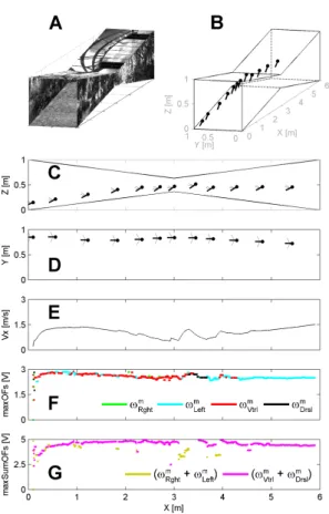
5.4. Automatic speed control in horizontally and/or vertically tapered tunnels 354

The simulated tunnels used here were 6-meter long, 1-meter high tapered 355

tunnels with a 1-meter wide entrance and a 0.25-meter constriction halfway 356

along the tunnel. This constriction could occur in either the horizontal plane 357

(Fig. 9A) the vertical plane (Fig. 10A), or both planes together (Fig. 11A). 358

These tunnels were designed to test the ability of the ALIS autopilot to 359

overcome several strong OF disturbances at the same time. 360

(FIGURE 9 and FIGURE 10 about here) 361

As shown in Fig. 9, the simulated bee was made to enter a tunnel with a 362

midway constriction in the horizontal plane, at the speed Vx0 = 0.2 m/sec and

363

with the initial coordinates x0 = 0.1 m, y0 = 0.85 m, z0 = 0.15 m (Fig. 9B).

364

Fig. 9C shows the trajectory in the vertical plane (x, z) and Fig. 9D in the 365

horizontal plane (x, y), plotted every 500 msec. 366

(21)

The simulated bee followed the left wall of the tapered tunnel, simply 367

because its starting point was close to that wall. The positioning criterion 368

(Fig. 9F) selected the left EMD output (ωm

lef t), which remained approximately

369

equal to the positioning OF set-point throughout the journey (Fig. 9F). The 370

simulated bee kept a safe left clearance throughout its journey. The simulated 371

bee automatically slowed down as it approached the narrowest section of the 372

tapered tunnel, and accelerated again when the tunnel widened out beyond 373

that point (Fig. 9E). Since the tunnel narrowed only in the horizontal plane, 374

the OF in the vertical plane was of little relevance to the speed control part 375

of the ALIS autopilot. The forward speed depended mostly on the OF in 376

the horizontal plane (ωm

Lef t+ ωRghtm , Fig. 9G) because the horizontal section

377

of the tunnel was smaller than its vertical section. 378

The ALIS autopilot made the simulated bee travel safely along the “hor-379

izontal” tapered tunnel (tapering angle 7 deg) without being greatly per-380

turbed by the major OF disturbance concomitantly detected by both its left 381

and right OF sensors. 382

As shown in Fig. 10, the simulated bee was then made to enter a tun-383

nel with a midway constriction in the vertical plane, at the speed Vx0 =

384

0.2 m/sec, with the initial coordinates x0 = 0.1 m, y0 = 0.85 m, z0 = 0.15 m

385

(Fig. 10B). Fig. 10C shows the trajectory in the vertical plane (x, z) and 386

Fig. 10D in the horizontal plane (x, y), plotted every 500 msec. In this case, 387

the simulated bee followed both the ground and the left wall of the tapered 388

tunnel, simply because its starting point was near to the ground and the 389

left wall. The positioning criterion could select either the ventral or left OF 390

measured (ωm

V tlr and ωLef tm ), which remained approximately equal to the

(22)

sitioning OF set-point throughout the journey (Fig. 10F). The simulated bee 392

kept a safe ventral and left clearance throughout its journey. 393

The simulated bee automatically slowed down as it approached the nar-394

rowest section of the tapered tunnel, and accelerated again when the tunnel 395

widened out beyond that point (Fig. 10E). As the tunnel narrowed only in 396

the vertical plane, the OF in the horizontal plane was of little relevance to 397

the speed control part of the ALIS autopilot. The forward speed depended 398

mostly on the OF in the vertical plane (ω_vtrlm + ωm_Drsl, Fig. 10G) because the 399

vertical section of the tunnel was smaller than its horizontal section. 400

The ALIS autopilot made the simulated bee travel along the vertically 401

tapered tunnel (tapering angle 7 deg) without being greatly perturbed by the 402

major OF disturbance concomitantly detected by both its ventral and dorsal 403

OF sensors. 404

As shown in Fig. 11, the simulated bee was then made to enter the tunnel 406

with midway constrictions in both the horizontal and vertical planes. The bee 407

entered at the speed Vx0= 0.2 m/sec with the initial coordinates x0 = 0.1 m,

408

y0 = 0.85 m, z0 = 0.15 m (Fig. 11B). Fig. 11C shows the trajectory in the

409

vertical plane (x, z) and Fig. 11D in the horizontal plane (x, y), plotted every 410

500 msec. The simulated bee followed both the ground and the left wall of 411

the tapered tunnel, simply because its starting point was near the ground 412

and the left wall. The positioning criterion could select either the ventral or 413

the left OF measured (ωm

V trland ωLef tm ), which remained approximately equal

414

to the positioning OF set-point throughout the trajectory (Fig. 11F). The 415

simulated bee kept a safe ventral and left clearance throughout its journey. 416

(23)

The simulated bee automatically slowed down as it approached the nar-417

rowest section of the tapered tunnel and accelerated again when the tunnel 418

widened out beyond this point (Fig. 11E). As the tunnel narrowed in both the 419

horizontal and vertical planes, the OFs in the horizontal and vertical planes 420

were both equally relevant to the speed control part of the ALIS autopilot. 421

The forward speed depended on the OFs in both the horizontal and vertical 422

planes (ωm

Rght+ ωLef tm and ωV tlrm + ωmDrsl, Fig. 11G) because the horizontal and

423

the vertical sections of the tunnel both varied to an equal extent. 424

The ALIS autopilot made the simulated bee cross the “horizontal and 425

vertical” tapered tunnel (tapering angle 7 deg in both planes) without being 426

greatly perturbed by a major overall OF disturbance concomitantly affecting 427

its lateral, ventral, and dorsal OF sensors. 428

All in all, these results show that the ALIS autopilot made the simulated 429

bee: 430

• adopt a cruise speed that will automatically adjust to whichever section 431

(horizontal or vertical) produces the largest optic flow, and 432

• adopt a clearance from one of the tunnel surfaces (the ground or the 433

roof or one wall) that will be proportional to the animal’s ground speed, 434

thus automatically generating both terrain-following and wall-following 435

behavior. 436

6. CONCLUSIONS 437

Here we have presented an OF-based 3D autopilot called ALIS. The re-438

sults of the computer simulations described above show that a simulated bee 439

(24)

equipped with the ALIS autopilot can navigate safely under purely visual 440

control along a straight tunnel (Fig. 6), occurs even when part of the wall or 441

the roof is devoid of texture (Fig. 7) and when the tunnel narrows or expands, 442

in either the horizontal or vertical plane (Fig. 8A, 9A, 10A), or in both planes 443

(Fig. 11A). Here we have not investigated dynamical disturbances such as 444

wind perturbations but tested ALIS’s robustness to strong OF perturbations. 445

Absence of contrast on one side (as Fig. 7) and tapered tunnels (Fig. 9- 11) 446

are considered by the ALIS control system (Fig. 4) as strong perturbations. 447

The autopilot manages to cope with these major perturbations, allowing the 448

simulated bee to fly safely in these tunnels. 449

These feats can all be achieved with a really minimalistic visual system 450

consisting of only eight pixels forming four EMDs (two EMDs in the hor-451

izontal plane and two in the vertical plane). The ALIS autopilot enables 452

the agent to avoid obstacles by performing maneuvers involving only trans-453

lational DOFs (along x, y, z). The key to the performances of the ALIS 454

autopilot is a pair of OF regulators designed to hold the perceived OF con-455

stant by adjusting the forward, side, and vertical thrusts. More specifically, 456

these two OF regulators operate as follows: 457

(i) The first OF regulator adjusts the bee’s forward speed so as to keep 458

whichever sum of the two opposite OFs (i.e., left+right or ventral+dorsal) 459

is maximum equal to a forward OF set-point. The outcome is that the bee’s 460

forward speed becomes proportional to the smallest dimension (width or 461

height, or both) of the corridor (Fig. 9E, 10E, 11E). Further simulations 462

showed (data not shown) that this occurs regardless of the position of the 463

bee’s starting point at the tunnel entrance. The forward speed attained by 464

(25)

the simulated bee depends also on the forward OF set-point ωsetF wd.

465

(ii) The second OF regulator adjusts the bee’s lateral and vertical position 466

so as to keep the largest OF value (from any of the four tunnel surfaces: walls, 467

ground, or roof) equal to the positioning OF set-point. The outcome is that 468

the clearance from the nearest wall (or ground or roof) becomes proportional 469

to the bee’s forward speed as defined in (i). The clearance from the nearest 470

tunnel surface depends on the positioning OF set-point ωsetP os.

471

The main advantage of this visuomotor control system is that it operates 472

efficiently without any needs for explicit speed or distance information, and 473

hence without any needs for speed or range sensors. The emphasis here 474

is on behavior rather than metrics: the simulated bee behaves appropriately 475

although it is completely “unaware” of its ground speed and its distance from 476

the walls, ground, and roof. The simulated bee navigates on the basis of two 477

parameters alone: the forward OF set-point ωsetF wd and the positioning OF

478

set-point ωsetP os (Fig. 4). The explicit ALIS control scheme presented here

479

(Fig. 4) can be viewed as a working hypothesis and is very much in line with 480

the ecological approach (Gibson, 1950), according to which an animal’s visual 481

system is thought to drive the locomotor system directly, without requiring 482

any “representation” of the environment (Franceschini et al., 1992; Duchon 483

and Warren, 1994). The ALIS control scheme (Fig. 4) readily accounts for the 484

behavior observed on real bees flying along a stationary corridor (Srinivasan 485

et al., 1991; Serres et al., 2008b; Baird et al., 2006) or a tapered corridor 486

(Srinivasan et al., 1996). It also accounts for the wall-following behavior 487

observed in straight or tapered corridors (Serres et al., 2008b). 488

Real bees have 4500 ommatidia, per eye and obviously more than four 489

(26)

OF sensors. These large number of OF sensors therefore enable them to 490

measure the OF in many directions and an elaborated autopilot could make 491

them to avoid obstacles occurring in many directions. An OF regulator is 492

little demanding in terms of its neural (or electronic) implementation since 493

it requires only a few linear operations (such as adding, subtracting, and 494

applying various filters) and nonlinear operations (such as minimum and 495

maximum detection). The minimalist control scheme described in this paper 496

could be implemented in a micro-controller running at 1kHz. In this way, 497

the “computation time” could be up to 1 msec. 498

In terms of the potential applications of these findings, biomimetic solu-499

tions of the kind described here may pave the way for the design of computation-500

lean, lightweight visual guidance systems for autonomous aerial, underwater, 501

and space vehicles. 502

ACKNOWLEDGMENTS 503

We thank S. Viollet and L. Kerhuel for their fruitful comments and sug-504

gestions during this work, R. Brinkworth and D. O’Carroll (Adelaide Uni., 505

Australia) for kindly making their panoramic images available to us, and J. 506

Blanc for improving the English manuscript. This work was supported partly 507

by CNRS (Life Science; Information and Engineering Science and Technol-508

ogy), by the Aix-Marseille University, by the French Defense Agency (DGA, 509

05 34 022), by the French Agency for Research (ANR, RETINAE project), 510

and by the European Space Agency (ESA) under contract n◦ 08-6303b. 511

(27)

References 512

Altshuler, D.L., Dickson, W.B., Vance, J.T., Roberts, S.P., and Dickinson, M.H. (2005). Short-amplitude

513

high-frequency wing strokes determine the aerodynamics of honeybee flight. PNAS. 102(50),

8213-514

18218.

515

Aub´epart, F., and Franceschini, N. (2007). A bio-inspired optic flow sensor based on FPGA: application

516

to micro-air-vehicles. J. of Microprocessors and Microsystems. 31(6), 408-419.

517

Baird, E., Srinivasan, M.V., Zhang, S., and Cowling, A. (2005). Visual control of flight speed in honeybees.

518

J. Exp. Biol. 208, 3895-3905.

519

Baird, E., Srinivasan, M.V., Zhang, S., Lamont, R., and Cowling, A. (2006). Visual control of flight speed

520

and height in honeybee. LNAI. 4095, 40-51.

521

Beyeler, A., Zufferey, J.-C., and Floreano, D. (2007). 3D vision-based navigation for indoor microflyers.

522

Proc. IEEE Int. Conf. on Robotics and Automation. pp. 1336-1341.

523

Blanes, C. (1986). Appareil visuel élémentaire pour la navigation à vue d’un robot mobile autonome. MS

524

in Neuroscience, Marseille, France: University of Aix-Marseille II.

525

Brinkworth, R.S.A., and O’Carroll, D.C. (2007). Biomimetic Motion Detection. Proc. of the Int. Conf. on

526

Intelligent Sensors, Sensor Networks and Information Processing (ISSNIP). 3, 137-142.

527

Coombs, D., and Roberts, K. (1992). Bee-bot: using peripheral optical flow to avoid obstacle. SPIE:

528

Intelligent robots and computer vision XI. 1825, 714-721.

529

David, C. (1978). The relationship between body angle and flight speed in free-flying Drosophila. Physiol.

530

Entomol. 3, 191-195.

531

Dickson, W.B., Straw, A.D., Poelma, C., and Dickinson, M.H. (2006). An integrative model of insect flight

532

control. Proc. of the 44th AIAA Aerospace Sciences Meeting and Exhibit. AIAA-2006-0034.

533

Dillon, M.E., and Dudley, R. (2004). Allometry of maximum vertical force production during hovering

534

flight of neotropical orchid bees (Apidae: Euglossini). J. Exp. Biol. 207, 417-425.

535

Duchon, A.P., and Warren, W.H. (1994). Robot navigation from a Gibsonian viewpoint. Proc. Int. Conf.

536

Syst. Man and Cyb. 2272-2277, San Antonio, Texas.

537

Dudley, R. (1995). Extraordinary flight performance of orchid bees (apidae: euglossini) hovering in heliox

538

(80% He / 20% O2_{). J. Exp. Biol. 198, 1065-1070.} 539

(28)

Dudley, R. (2000). The biomechanics of insect flight: form, function, evolution, (Princeton: Princeton

540

University Press).

541

Ellington, C.P. (1984). The aerodynamics of hovering insect flight. III. Kinematics. Phil. Trans. Roy. Soc.

542

Lond. B. 305, 41-78.

543

Esch, H., Nachtigall, W., and Kogge, S.N. (1975). Correlations between aerodynamic output, electrical

544

activity in the indirect flight muscles and wing positions of bees flying in a servomechanically controlled

545

flight tunnel. J. Comp. Physiol. 100, 147-159.

546

Franceschini, N., Pichon, J.M., and Blanes, C. (1992). From insect vision to robot vision. Philos. Trans.

547

R. Soc. Lond. B 337, 283294.

548

Franceschini, N., Ruffier, F., and Serres, J. (2007). A bio-inspired flying robot sheds light on insect piloting

549

abilities. Current Biology. 17, 329-335.

550

Franceschini, N., Ruffier, F., Serres, J., and Viollet, S. (2009). Optic flow based visual guidance: from

551

flying insects to miniature aerial vehicules. In Aerial Vehicles, T.M. Lam, ed. (In-Tech), pp. 747-770.

552

von Frisch, K. (1948). Gelöste und ungelöste Rätsel der Bienensprache. Naturwissenschaften. 35, 38-43.

553

Gibson, J.J. (1950). The perception of the visual world. (Boston: Houghton Mifflin).

554

Horridge, G.A. (1987). The evolution of visual processing and the construction of seeing system. Proc.

555

Roy. Soc. Lond. B. 230, 279-292.

556

Humbert, J.S., Hyslop, A., and Chinn, M. (2007). Experimental validation of wide-field integration

meth-557

ods for autonomous navigation. Proc. IEEE int. conf. intelligent robots and systems.

558

Ibbotson, M.R. (2001). Evidence for velocity-tuned motion-sentive descending neurons in the honeybee.

559

Proc. Roy. Soc. Lond. B. 268, 2195-2201.

560

Lewis, M.A. (1997). Visual Navigation in a Robot using Zig-Zag Behavior, NIPS.

561

Nachtigall, W., Widmann, R., and Renner, M. (1971). Uber den ortsfesten freien Flug von Bienen in

562

einem Saugkanal. Apidologie. 2, 271-282.

563

Netter, T., and Franceschini, N. (2002). A robotic aircraft that follows terrain using a neuromorphic eye.

564

Proc. IEEE int. conf. intelligent robots and systems. 129-134.

565

Neumann, T.R., and B¨ulthoff, H.H. (2001). Insect visual control of translatory flight. LNCS/LNAI. 2159,

566

627-636.

(29)

Pichon, J.M., Blanes, C., and Franceschini, N. (1989). Visual guidance of a mobile robot equipped with a

568

network of self-motion sensors. Proc. SPIE 1195, 44-53.

569

Preiss, R. (1987). Motion parallax and figural properties of depth control flight speed in an insect. Biol.

570

Cyb. 57, 1-9.

571

Pudas, M., et al. (2007). A miniature bio-inspired optic flow sensor based on low temperature co-fired

572

ceramics (LTCC) technology. Sensors and Actuators A. 133, 88-95.

573

Riley, J.R., et al. (2003). The Automatic Pilot of Honeybees. Proc. Roy. Soc. Lond. 270, 2421-2414.

574

Ruffier, F., and Franceschini, N. (2003). Bio-inspired optical flow circuits for the visual guidance of

micro-575

air vehicles. IEEE int. symp. circuits and systems. 3, 846-849.

576

Ruffier, F., and Franceschini, N. (2005). Optic flow regulation: the key to aircraft automatic guidance.

577

Robotics and Autonomous Systems. 50(4), 177-194.

578

Sane, S.P., and Dickinson, M.H. (2002). The aerodynamic effects of wing rotation and a revised

quasi-579

steady model of flapping flight. J. Exp. Biol. 205, 1087-1096.

580

Santos-Victor, J., Sandini, G., Curotto, F., and Garibaldi, S. (1995). Divergent stereo in autonomous

581

navigation: from bees to robots. Int. J. of Comp. Vision. 14, 159-177.

582

Schilstra. C., and van Hateren, J.H. (1999). Blowfly flight and optic flow. I. Thorax kinematics and flight

583

dynamics. J. Exp. Biol. 202, 1481-1490.

584

Seidl, R., and Kaiser, W. (1981). Visual field size, binocular domain and the ommatidial array of the

585

compound eyes in worker honey bees. J. Comp. Physiol. A 143, 1726.

586

Serres, J., Dray, D., Ruffier, F., and Franceschini, N. (2008). A vision-based autopilot for a miniature

587

air-vehicle: joint speed control and lateral obstacle avoidance. Autonomous Robot. 25, 103 -122.

588

Serres, J., Ruffier, F., Masson, G.P., and Franceschini, N. (2008). A bee in the corridor: centering and

589

wall-following. Naturwissenschaften. 95, 1181-1187.

590

Srinivasan, M.V., Lehrer, M., Kirchner, W.H., and Zhang, S.W. (1991). Range perception through

appar-591

ent image speed in freely flying honeybees. Vis. Neurosci. 6, 519-535.

592

Srinivasan, M.V., Zhang, S.W., Lehrer, M., and Collett, T.S. (1996). Honeybee navigation en route to the

593

goal: visual flight control and odometry. J. Exp. Biol. 199, 237-2446.

594

Srinivasan, M.V., Zhang, S.W., Chahl, J.S., Barth, E., and Venkatesh, S. (2000). How honeybees make

595

grazing landings on flat surfaces. Biol. Cyb. 83, 171-183.

(30)

Tammero, L.F., and Dickinson, M.H. (2002). Collision-avoidance and landing responses are mediated by

597

separate pathways in the fruit fly, Drosophila melanogaster. J. Exp. Biol. 205, 2785-2798.

598

Vickers, N.J, and Baker, T.C. (1994). Visual feedback in the control of pheromone-mediated flight in

599

Heliothis virescens males (Lepidoptera: noctuidae). J. Insct. Behav. 7, 605-631.

600

Wakakuwa, M., Kurasawa, M., Giurfa, M., and Arikawa, K. (2005). Spectral heterogeneity of honeybee

601

ommatidia. Naturw. 92, 464-467.

602

Weber, K., Venkatesh, S., and Srinivasan, M.V. (1997). Insect inspired behaviours for the autonomous

603

control of mobile robots, M.V. Srinivasan and S. Venkatesh, Eds. From living eyes to seeing machines.

604

(Oxford: Oxford University Press).

605

Zeil, J., Boeddeker, N., and Hemmi, J.M. (2008) Visualy guided behavior. In New Encyclopedia of

Neu-606

roscience (Amsterdam: Elsevier Science Publishers), in press, 2008.

607

Zufferey, J.-C., and Floreano, D. (2005). Toward 30-gram autonomous indoor aircraft: vision-based

obsta-608

cle avoidance and altitude control. Proc. IEEE Int. Conf. on Robotics and Automation. pp. 2594-2599,

609

Barcelona, Spain.

(31)

Figure 1: (A) Resolution of the mean flight-force vector ~F along the surge X-axis giving the forward thrust T , along the sway Y-axis giving the side thrust S, and along the heave Z-axis giving the vertical lift L. (B) Pitching the mean flight-force vector ~F by an angle θpitchgenerates a forward thrust T . (C)

Rolling the mean flight-force vector ~F by an angle θrollgenerates a side thrust S.

Figure 2: The grayscale natural scenes used to line the 4 internal faces of the simulated tunnel. Resolution of the images was 1000×6000 pixels (1 pixel = 1 mm2_{). Images are therefore 1×6-meter in size. All four}

faces of the tunnel were lined with different images: right wall (A), left wall (B), roof (C), and ground (D).

(32)

Figure 3: (A) A simulated bee flying at forward speed Vx along a tunnel generates an OF (Eq. 8)

that depends on the perpendicular distance (right DRght, left DLef t, ventral DV trl, dorsal DDrsl) from

the tunnel surfaces. The simulated bee is equipped with four OF sensors. The sensors’axes are always oriented at fixed roll and pitch orientations, perpendicular to the walls, ground and roof, respectively, and the OF is generated laterally (ωLef tand ωRght), ventrally (ωV trl) and dorsally (ωDrsl). (B) Each OF

sensor consists of only two photoreceptors (two pixels) driving an Elementary Motion Detector (EMD). The visual axes of the two photoreceptors are separated by an interreceptor angle ∆ϕ = 4 deg.

(33)

Figure 4: The ALIS autopilot is based on two interdependent visual feedback loops, each with its own OF set-point: a speed control loop (in blue) and a positioning control loop (in red). The surge controller adjusts the pitch angle θpitch(that determines Vxvia the bees’ surge dynamics) on the basis of whichever

sum of the two coplanar (horizontal or vertical) OFs measured is the largest. This value is compared with the forward OF set-point ωsetF wd. The surge controller commands the forward speed so as to minimize

the error εF wd. The positioning controller controls the roll angle θroll (or the stroke amplitude ∆Φ ),

which determines the distances to the walls (or the distances to the ground and to the roof), depending on the sway (or heave) dynamics on the basis of whichever of the four measured OFs is the largest. The latter value is compared with the positioning OF set-point ωsetP os. At any time, the direction of avoidance is

given by a Control direction Selector that multiplies the control signal by a direction factor depending on the direction of the maximum OF signal (see Fig. 5). The positioning controller (Proportional-Derivative, PD) commands the sway (or heave) dynamics so as to minimize the error εP os. The dash accross the

connection lines indicates the number of variables involved. Diis the distance to the surface involved (see

(34)

Figure 5: The Control direction Selector automatically selects the tunnel surface to be followed (wall, ground or roof) by multiplying the control signal (the output from the Positioning controller) by a direction factor that depends on the direction of the largest OF signal. Note that the sway and heave dynamics can be driven alternately, depending on which OF (side or vertical) is the largest at any given time. The input to the sway or heave dynamics that is not relevant is set to zero. In the example shown here, the direction of the maximum OF is “right”. Consequently, the output for the Side thrust is the control signal multiplied by -1 and the output for the Vertical thrust is the control signal multiplied by 0.

(35)

Figure 6: (A) Perspective view of the straight flight tunnel. (B) Simulated bee’s 3-D trajectory starting at x0 = 0.1 m, with initial speed Vxo = 0.2 m/sec, and various y0 and z0, plotted every 500 msec. (C)

Trajectory in the vertical plane (x, z), every 500 msec. (D) Flight track in the horizontal plane (x, y), plotted every 500 msec. (E) Forward speed Vxprofile.

(36)

Figure 7: (A) Perspective view of the straight flight tunnel including two ”no contrast” zones. (B)Simulated bee’s 3-D trajectory starting at x0 = 0.1 m, y0 = 0.85 m, z0 = 0.85 m, at the forward

speed Vxo= 0.2 m/sec, plotted every 500 msec. (C) Trajectory in the vertical plane (x, z), every 500 msec.

(D) Trajectory in the horizontal plane (x, y), plotted every 500 msec. (E) Forward speed Vxprofile. (F)

Positioning feedback signal determined by the largest output from the four OF sensors (right OF sensor = green; left OF sensor = cyan; ventral OF sensor = red; dorsal OF sensor = black). (G) Forward feedback signal determined by the largest sum of the two diametrically opposed OF sensors (horizontal OF sensors = yellow; vertical OF sensors = magenta).

(37)

Figure 8: (A) Perspective view of the tapered tunnel. (B) Simulated bee’s 3-D trajectory starting at the initial coordinates x0= 0.1 m, y0= 0.75 m, z0= 0.25 m, and at the speed Vxo= 0.2 m/sec, plotted every

500 msec. (C) Trajectory in the vertical plane (x, z), every 500 msec. (D) Trajectory in the horizontal plane (x, y), plotted every 500 msec. (E) Forward speed Vxprofile. (F) Positioning feedback signal determined

by the largest output from the four OF sensors (right OF sensor = green; left OF sensor = cyan; ventral OF sensor = red; dorsal OF sensor = black). (G) Forward feedback signal determined by the largest sum of the two diametrically opposed OF sensors (horizontal OF sensors = yellow; vertical OF sensors = magenta).

(38)

Figure 9: (A) Perspective view of the tapered tunnel. (B) Simulated bee’s 3-D trajectory starting at the initial coordinates x0= 0.1 m, y0= 0.85 m, z0= 0.15 m, and at the speed Vxo= 0.2 m/sec, plotted every

(39)

Figure 10: (A) Perspective view of the tapered tunnel. (B) Simulated bee’s 3-D trajectory starting at the initial coordinates x0 = 0.1 m, y0 = 0.85 m, z0 = 0.15 m, and at the speed Vxo = 0.2 m/sec,

plotted every 500 msec. (C) Trajectory in the vertical plane (x, z), every 500 msec. (D) Trajectory in the horizontal plane (x, y), plotted every 500 msec. (E) Forward speed Vxprofile. (F) Positioning feedback

signal determined by the largest output from the four OF sensors (right OF sensor = green; left OF sensor = cyan; ventral OF sensor = red; dorsal OF sensor = black). (G) Forward feedback signal determined by the largest sum of the two diametrically opposed OF sensors (horizontal OF sensors = yellow; vertical OF sensors = magenta).

(40)

Figure 11: (A) Perspective view of the tapered tunnel. (B) Simulated bee’s 3-D trajectory starting at initial coordinates x0= 0.1 m, y0= 0.85 m, z0= 0.15 m, and at the speed Vxo= 0.2 m/sec, plotted every