Delay in reporting Acquired Immune Deficiency Syndrome (AIDS)

Digitized

by

the

Internet

Archive

in

2011

with

funding

from

Boston

Library

Consortium

Member

Libraries

working

paper

department

of

economics

DELAY IN REPORTING

ACQUIRED IMMUNE DEFICIENCY SYNDROME (AIDS)

Jeffrey E. Harris No. 452 May 1987

massachusetts

institute

of

technology

...

memorial

drive

Cambridge, mass.

02139

DELAY IN REPORTING

ACQUIRED IMMUNE DEFICIENCY SYNDROME (AIDS)

Jeffrey E. Harris

May 1987

Delay in Reporting

Acquired Immune Deficiency Syndrome (AIDS)

by

Jeffrey E. Harris*

ABSTRACT

As of March 31, 1987, the U.S. Centers for Disease Control had reported 33,350 cases of acquired immune deficiency syndrome. Yet by that date, physicians

had actually diagnosed 42,670 cases. The difference arises from significant delays in the reporting of AIDS cases to public health authorities. An

estimated 70% of cases are reported two or more months after diagnosis; about

23% are reported seven or more months later; and about 5% take more than three years to come in. Moreover, the probability distribution of delays has been shifting to the right, with the median delay increasing by 0.6 months since mid-1986. From the data on reported cases and the estimated probability distribution of reporting delays, I reconstruct the actual incidence of AIDS from January 1982 through March 1987. The doubling time of the epidemic fell

from about 6 months in 1982 to 15-16 months in 1986.

KEYWORDS: empirical distribution; truncated data; EM algorithm;

non-parametric models; semi-parametric models; epidemic; incidence.

*Massachusetts Institute of Technology and Massachusetts General Hospital. Address reprint requests to the author at Massachusetts Institute of

Technology, Department of Economics, E52-252g, Cambridge, Massachusetts

02139. I gratefully acknowledge the assistance of the AIDS Program at the

Centers for Disease Control, especially Dr. V. Meade Morgan and Kathy Winter. The contents this paper are my sole responsibility.

-2-1. INTRODUCTION

As of March 31, 1987, the U.S. Centers for Disease Control (CDC) had reported 33,550 cases of acquired immune deficiency syndrome (AIDS). Yet by that date, I estimate, physicians had actually diagnosed 42,670 cases.

The difference arises from significant delays in the reporting of AIDS cases to public health authorities. Some 9,120 additional persons had already been stricken with the disease, but they were not yet part of the CDC's

official tally.

In this paper, I derive the empirical distribution of AIDS reporting delays and test its stationarity. From my results on reporting delays and the

data on reported cases, I then estimate the actual incidence of the disease. While CDC reported about 4,500 new AIDS cases during the first calendar quarter of 1987, I find the incidence to be about 5,600.

Reporting delays are not the only reason why CDC's listings may fall short of the actual counts. Some cases of AIDS may never be reported. Doctors may be loath to inform public health authorities about certain patients. Also, the CDC's case definition of AIDS has not included all

serious consequences of infection by the human immunodeficiency virus. These forms of underreporting, which can be viewed as reporting delays of infinite length, _{have been studied elsewhere (Chamberland} et al. 1985; CDC 1986ab) and will not be my main focus here.

While researchers have attempted to adjust for reporting delays (Curran

et al. 1985; Morgan and Curran 1986), the present paper appears to be the

first formal analysis of the problem. Some of this paper's findings have been noted in an earlier report (Harris 1987).

2. THE PROBLEM

Once an individual is stricken with AIDS, the fact of his or her diagnosis is not instantly known to the CDC. Two more events need to take place. First, the attending physician or hospital reports the case to the

local or state health department. Second, the health department transmits the

information to the CDC.

The first step relies upon a surveillance system that is essentially passive. Although health departments in a few states actively review hospital and clinic records, most merely wait for the reports to come in. The second step entails periodic mailings by the health departments to the CDC. Starting

in April 1986, the health departments switched from typewritten case reports

to floppy diskettes, which were computer-encoded at the departments. By August 1986, most departments were mailing the diskettes.

• For each reported case, the CDC lists both the date of diagnosis and the

date of report. Up to March 1983, the date of report meant the time the

health department received the information. Thereafter, the reporting date meant the time when the CDC received the data, that is, when both steps had been completed.

Among the 33,350 cases reported through March 1987, 336 were diagnosed during 1981. Of these, only 201 were actually reported during that year. Another 74 were reported in 1982, and 15 were not reported until 1986 or

later.

For the 336 cases diagnosed in 1981, the records do not show the specific month of diagnosis. I shall therefore analyze the remaining 33,214 cases

-4-reported from January lr 1982 through March 31, 1987

—

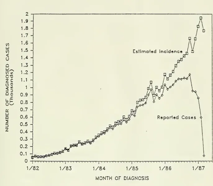
for which the records do provide both the month and year of diagnosis.

Figure 1 shows the frequency distribution of these cases according to

their date of diagnosis. The number of diagnosed cases falls off sharply

after October 1986. But this does not mean that the incidence of the AIDS has

been falling. Many cases diagnosed in late 1986 or early 1987 may not have been reported by March 1987.

In order to estimate the actual incidence of AIDS, we need to recover the

unreported cases, and that requires estimating the distribution of reporting

delays. In particular, we need to know the distribution of delays among all

diagnosed cases, not just among the ones reported so far. This is because the

delays observed for the reported cases constitute a truncated sample from the actual distribution. The question then becomes: What minimum assumptions are

required to estimate the distribution of reporting delays?

3. STATISTICAL METHODS

3.1. Notation. Divide the time axis into intervals of equal length, called "periods," indexed by the positive integers. A new case of AIDS

diagnosed during period t may not be reported until period t+u, where the non-negative integer u denotes the duration of the reporting delay. For short hand, I use the phrase "at t" to mean "during period t," while "by t" means

"at any time up to the end of period t."

Let T be a known, nonrandom positive integer. Among all cases diagnosed

by T, we observe only those reported by T. That is, for any case in which t+u

(0

u

V)

<

o

Q

•-S

°5

0. °

*o

U.-C LU CD

D

Z

1/82 1/83

1/84

1/85 1/86

MONTH

OF DIAGNOSIS

FIGURE 1. Distribution of 33,214 AIDS Cases Reported to the CDC through March 31, 1987 According to Month of Diagnosis. (Not shown in the

•5-cases for which t £ T but t+u > T. From such truncated data, we wish to

estimate the actual number of cases diagnosed at each t £ T.

Let yt (u) signify the number of cases diagnosed at t and reported at

t-t

t+u. Define yt =

X

yt (u) as the number of cases diagnosed at t and reported

U

-T-U

by T. Let y(u) = 21 yt (u) be the number reported with delay u, and define

t= o

_ T

y = 21 yt as the total number of reported cases. Let Y denote the set of all

yt (u) , and y the set of all yt .

Let

m

(u) denote the probability that a case of AIDS, diagnosed at t,

t-t

will be reported with delay u. Define 6t = 21

m

(u) to be the probability that

U =

a case of AIDS, which has been diagnosed at t, will be reported by T. The symbol n will denote all

m

(u) and, by implication, all St.

3.2. Basic Model. Denote by xt the number of cases diagnosed at t,

whether or not they are reported by T. The counts xt are unobserved.

Assumption I (Non-Parametric Model of AIDS Incidence): For all t, the

counts xt of diagnosed cases are independently Poisson distributed, with

respective means At . Each At is termed the "incidence at t." Let A represent

the set of all At

.

If a case of AIDS is diagnosed at t and reported by T, then it will be

reported at t+u with probability nt(u)/6t . Therefore, given the marginal

sums yt and the parameters

m

(u) and 9t , the joint distribution of the counts

-6-yt!

^r

yt(u)

(Y|y,n) = i

f ] j tm(u)/et]

t=1 yt(0)! ••• yt(T-t)! u=0

Moreover, given xt and 6t for each t, the counts yt are independently

binomially distributed as b(yt|xt,8t). By Assumption I, each xt is Poisson distributed with mean At. Hence, given At and 8t , each yt is Poisson

distributed with mean 6t At . Given parameters

m

(u) and At, the joint

distribution of the marginal sums yt is

yt

h(y|n,A) = j |

[GtAt] exp[-8t At]/yt

t=i

The likelihood of the parameters rr and A is thus the product of expressions

g(Y|yfn) and h(y|n,A). Up to an additive constant, the log-likelihood

function is

T

T-t

T

L(tt,A) = 51 51 yt (u)ioo-(nt (u)/8t) + :£ [yt logiBiAt ) - 8tAt] (1) .

t=1 u= ' t=l

Now consider the concentrated log-likelihood L* (rr) . That is, for arbitrarily fixed tt, we choose A = A*(rr) to maximize L(n,A) and then define

L*(n) = L(tt, A* (n) ) . From (1), it is apparent that At*(n) = yt /8t . Up to an

additive constant, the concentrated log-likelihood is therefore

L*(TT) = 21

T

±

Vt (u)ioer(TTt (u)/8t)

-7-Assumptiop II (Stationarity of Reporting Delay Distribution): The

probability distribution of reporting delays is independent of the date of

diagnosis. That is,

m

(u) = tt(u) for all t,u.

M

It will prove convenient to define S(v) = IE rr(u) , the right-hand tail

U=V

of the reporting delay distribution. If we permit n to be a defective

distribution, then the tail s(v) equals the probability of finite reporting

delays of v or more periods plus the probability that a case may never be

reported. The concentrated log-likelihood function is now

T-l T

L*(n) =

X

y(u)iogr tt(u) -

H

ytlogBt

(2),

u= o t=1

which is homogeneous of degree zero in the arguments n(0) , tt(T-I). That is, from Assumptions I and II alone, we can identify the probabilities

n(0),

—

,n(T-l) only up to a proportionality constant. To solve this problem,

we could impose a parametric form of the entire distribution n(u) . Instead, I shall assume that we have prior information on S(T), the proportion of

diagnosed cases that will go unreported for T or more periods.

Constrained maximization of L* (n) in (2) can be achieved by the following

iterative procedure, analogous to the EM algorithm (Dempster, Laird and Rubin 1977). Consider estimates n(K) (u) obtained at the Nth stage in the iteration

t- t

and define 6t<N

> = 11 n(K>(u) for each _t. Given _6t (

N

)

, the maximum likelihood

u =

estimate of Xt is Xt <K> = yt/Gt<N >. To obtain n (K+1) _(u) at the N+ls t stage,

-8-p(u) = y(u)/ _Je Xt<"> (3),

for each u, and then normalize the values of p(u) in (3) to sum to l-S(T)

n<N+i>{_u

) = [i-s(T)]p(u) /

r

£: p(p) (4)

V=

An appropriate starting value is tt(1> (u) = (l-S(T) )y(u)/y.

3.3. Variants of the Basic Model. Consider the following alternative to

Assumption I.

Assumption IA (Parametric Model of AIDS Incidence): For all t, the

counts xt are independently Poisson distributed with respective means

/(t,E)/g, where a is a scale parameter and & is a vector of other parameters. Conditional upon 8t , a and (5, the counts yt are now independently Poisson

distributed with means 8t/(t,|S)/a. Under Assumptions IA and II, the log-likelihood function becomes

L(n,a,p) =

T

il y(u)Jog [n(u)/a] +

£

yxlofffit,}) -

_Z*

_[n(u)/a]

_z"

_{/(t,p) (5)}

u=0 t=l u=0 t=l

L(n,a,P) is homogeneous of degree zero in the arguments a,n(0) , . . .n(T-l) .

Hence, we still need an identifying restriction on either the scale a of the

epidemic or the proportion £(T) of cases reported with delays of T or more. When we have prior information on £(T), we can maximize L(n,a,p) by an

interative procedure analogous to (3) and (4). Consider estimates n<N_>(u)

obtained at the Nth stage of the iteration. Given rr(K) (u), we estimate a(K>

and p<K> _{by maximization}

-9-T-u

obtain the N+lsl _{values of n(u) by computing p(u)} = y(u)a< N_{>/:E /(t,p<}K _>)

t=

for each u, and then (given S(T)) applying the normalization (4).

Let T' be a known positive integer for which T' < T, and consider the

following alternative to Assumption II.

Assumption IIA (Non-Stationarity of Reporting Delay Distribution) : All cases of AIDS diagnosed by T' have an identical probability distribution n(u) of reporting delays. Those cases diagnosed after T' also have an identical,

but possibly different distribution n'

(u) of reporting delays.

Under Assumptions I and IIA, we obtain a concentrated log-likelihood

function that is a generalization of (2). In that case, L(tt,tt') is

homogeneous of degree zero in the arguments n(0) , . . . ,n(T-l) and separately in

the arguments TT

1

(0) , .. .,TT' (T-T'-l) . Hence, we need two restrictions to

identify the parameters: one on S(T), the right-hand tail of it; and

another-on S'(T-T'), the right-hand tail of rr'.

Alternatively, under Assumptions IA and IIA, we obtain a log-likelihood function that is a generalization of (5). In that case, L(n,n',a,P) is

homogeneous of degree zero in the combined arguments n(0) ,

—

,n(T-l) ,

n' (0) ,... ,n' (T-T'-l)., and a. Only a single restriction (such as on a, S(T) or

S'(T-T') ) is sufficient to identify the parameters.

Assumption IIA is only the simplest case of non-stationarity. In

principle, we could partition the time axis into more than two intervals, with boundaries T', T", etc., and specify a different reporting delay distribution

(rr, tt', TT", etc.) for each interval. If we continue to maintain Assumption I,

-10-corresponding tail probabilities S(T), S'(T-T'), S"(T-T"), etc. In

particular, in the computations reported below, I shall assume that £(T) = 0;

and further that the tails of successive distributions are "matching," that

is, S'(T-T') = S(T-T'), S"(T-T") = 8' (T-T"), etc. In practice, this means

that we first compute the estimates ft(0) , . . . ,ft(T-l) under the restriction

that S(T) = 0. Ve then compute ft' (0) , . . . ,fr* (T-T 1

) under the restriction

S'(T-T') = ft(T-T') + ••• + ft(T-l); then estimate ft"(0) , .. . ,ft" (T-T")

under the restriction S"(T-T") = ft' (T-T") + ••• + ft' (T-T'+l) + S'(T-T');

and so forth.

Under Assumptions IA and

HA,

however, we still require only a single identifying restriction. In particular, in the results below, I shall assume that min I S(T) ,

S

' (T-T' ) ,S" (T-T") , . . . I = 0.

3.4. Remarks. In the basic model (Assumptions I and II), the

concentrated log-likelihood L* (n) in (2) has T unknown parameters.

Alternatively, under Assumptions IA and II, the full log-likelihood L(n,a,p)

in (5) entails at least T+2 unknown parameters, and under Assumptions IA and

HA,

the generalization L(n,n',a,P) entails at least 2T+T'+2 parameters. In

each case, the maximum likelihood estimates of the parameters are consistent

and asymtotically efficient as the number of reported cases y grows large,

provided that the counts yt grow faster than T.

Under Assumption I, we have posited what amounts to a null model of the

AIDS epidemic. Hence, we can estimate the reporting delay parameters n (at

least up to a proportionality factor) from the concentrated log-likelihood

L*(tt) in (2). Under Assumption IA, by contrast, the parametric model of AIDS

-11-case, the log-likelihood L(u,a,f>) in (5) cannot always be concentrated in a

simple way, and the delay distribution n and the incidence model /(t,P)/a thus have to be estimated jointly.

Even when we have a specific model for AIDS incidence, the function L* (n) can still be interpreted as a partial likelihood in the sense of Cox (1975).

Suppose that each count xt has unspecified probability distribution k(xt|t,<t>),

which depends on the set <t> of parameters and which is not necessarily Poisson.

The log-likelihood function can be written

L(TT,<t>) = L*(tt) + i: log [i: b(yt |x,6t) -kUlt,*)] ,

t=1 X =

where b(yt|x,6t) is the binomial distribution. Even if we were informed about

the AIDS epidemic model k(xt|t,0), the dimensionality of could be so large that we might want to treat <D essentially as a set of

nuismce

parameters and

estimate tt from L*(n) alone.

4. RESULTS

4.1. Non-Parametric Model of AIDS Incidence. Figure 2 compares the

distribution of reported cases with the estimated incidence of AIDS. The curve denoted Reported Cases, reproduced from Figure 1, corresponds to the

counts yt . The curve denoted Estimated Incidence corresponds to the estimates

of Xt under Assumption I, where we posit no parametric model of the epidemic.

As Figure 2 shows, a significant fraction of AIDS cases had not been reported by March 31, 1987, even among those diagnosed in early 1986. For example, 1,037 AIDS cases were reported as diagnosed in January 1986. Yet

V)

u

10 < u

Q

CO M 0-0 Z C

o

o

<3

, .c

u

m

2

D

2

1/82

1/83

1/84

1/85

MONTH

OF DIAGNOSIS 1/86

1/87

FIGURE 2. Estimated Incidence of AIDS Compared to Number of Diagnosed

Cases Reported through March 31, 1987. (The curve of "Reported Cases"

is duplicated from Figure 1. The "Estimated Incidence" curve was

-12-Figure 2 gives an estimated incidence of 1,175 in that month, with the

approximate lower and upper 95% confidence bounds (not given in the Figure) of

1,120 and 1,242. Similarly, 855 AIDS cases were reported as diagnosed in

January 1987, yet the estimated incidence is 1,829 with 95% confidence bounds

of 1,730 and 1,959. (I computed the confidence bounds by the bootstrap method

of Efron (1979) , where repeated draws were made from the empirical

distribution of the counts yt(u).)

In the computations of Figure 2, I allowed for non-stationarity in the

reporting delay distribution n (that is, Assumption IIA) . In doing so, I

partitioned the observation period (January 1982-March 1987) into four

intervals: (1) January 1982-March 1983, when the encoded date of report was

actually the date of receipt by the health department; (2) April 1983-March

1986, when the date of report was changed to the date received by CDC; (3)

April-August 1986, when the health departments switched to computer-encoded

diskettes; and (4) September 1986-March 1987, when the current reporting

system was in place. Numbering successive months from January 1982 to March

1987 as t = 1, ,63, we thus have T' = 15, T" = 51 and T"' = 56. There

are four potentially different reporting delay distributions, n, n' , tt" and

n"\

identified by restrictions on S (63) , S'(48), S"(12) and £'"(7).

The "matching tails" restrictions, in particular, mean that S(63) = 0, £'(48) =

SUB),

£"(12) = £'(12) and £'"(7) = £"(7).

Significant non-stationarity in the reporting delay distribution was found. The estimated proportions of cases reported within the same month

were: fr(0) = 0.287; fr' (0) = 0.059; fr"(0) = 0.088; and fi'"(0) =

-13-subsequent month (that is, n(0)+n(l) ) were respectively: 0.491, 0.350, 0.367,

and 0.305. Allowing for n # n' (but retaining the restrictions n' = n" =

n'") added 48 parameters but increased the log-likelihood by 422.0 (P <

0.0001 by the chi-squared test). Allowing for n # n' and n1

/ n" (but

retaining n" = n'") added 12 more parameters but increased the

log-likelihood by 14.8 (P < 0.005). The completely unconstrained model added 7 more parameters with a further log-likelihood increase of 68.6 (P < 0.0001).

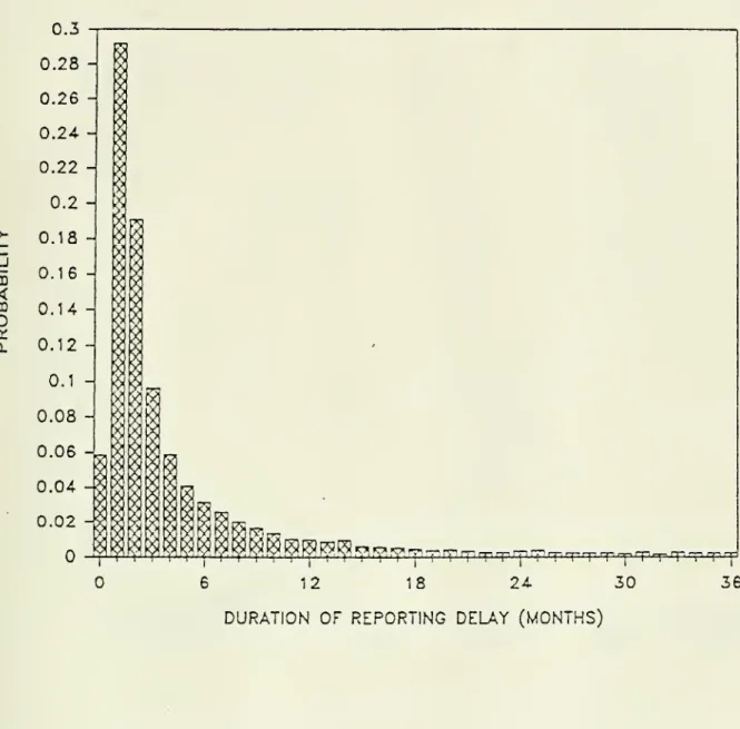
Figure 3 shows the estimated distribution ft' for cases diagnosed during

April 1982-March 1986 (interval 2). The distribution fits neither a Poisson nor a negative binomial. Up to about 18 months, ft' approximately follows a

Pareto rule (that is, the probability of reporting delays in excess of u

months is approximately proportional to u-0 - 85 ).

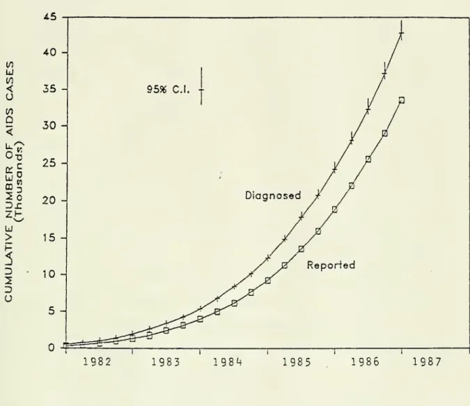
Figure 4 shows the cumulative number of diagnosed and reported AIDS cases by calendar quarter, based upon the results given in Figure 2. A total of

33,350 cases had been reported by March 31, 1987 (including those reported in

1981). Yet by that date, an estimated 42,670 had been diagnosed (95%

confidence bounds 41,736 and 44,399). While the CDC had reported 4,523 new cases during the first quarter of 1987, I estimate that 5,542 were actually diagnosed (95% confidence bounds 5,180 and 6,044).

4.2. Parametric Models of the Epidemic. The estimated incidence curve

in Figure 2 is not exponential. The doubling time of the epidemic, which appears to have been about 6 months in 1982, fell to about 9-10 months in 1984

and 15-16 months in 1986. While a subexponential epidemic may be plausible,

the validity of the doubling-time estimates hinges on the "matching tails" restrictions on S(T), S'(T-T'), s"(T-T") and S"'(T-T"'). Since

0.3

>-H

_J CD

<

m

o

tx. 0. Mr^rf^^r^rprp,^p,rprprr,

T

:rrrrrpi

T

irr,nprrqnn! -6 12 18 24 30

DURATION OF REPORTING DELAY (MONTHS)

36

FIGURE 3. Estimated Probability Distribution of Reporting Delays for

AIDS Cases _{Diagnosed During April 1983-March 1986. (The estimated}

CO

u

CO <

o

CO

Q

PI

U

m

Dl

ZH->

D

U

1982 1983

1984

1985

1986

1987

FIGURE 4. Estimated Cumulative Incidence of AIDS Compared to Cumulative

Reported Cases, First Quarter of 1982 through First Quarter of 1987.

(Approximate 95 percent confidence intervals are given for the

-14-these restrictions remain untested, the confidence intervals in Figure 4 understate the degree of uncertainty in the estimated size of the epidemic.

For instance, the "matching tail" assumption meant that £'(48) = 0.032,

S"(12) = 0.146, and S'"{7) = 0.233. The last restriction means that

among cases diagnosed during September 1986-March 1987, 76.7 percent would be the reported within 6 months of diagnosis. But if we arbitrarily changed

S'"(7) to 0.5, then the estimated incidence in the first quarter of 1987

would jump from 5,600 to 8,500 cases, while the total number of diagnosed

cases would stand at 49,000.

As a means of validating the results of Figures 2, 3 and 4, I tested a

flexible parametric model of the epidemic (Assumption IA) . Specifically, I assumed that the counts xt were independently Poisson distributed with respective means equal to exp [$o + pit + ($2t2 + f.3

1

3

] . Such a functional form was used not for any theoretical appeal, but simply as a means of

smoothly approximating the path of the epidemic thus far. The resulting

estimates of n, tt

1

, tt" and rr"' (and the corresponding tails) were

virtually identical to those in Section 4.1. The fitted incidence model was exp [3.723 + 0.118t - _1.44xl0-3_t2 _{+ 8}

.28xl0"6t3]

.

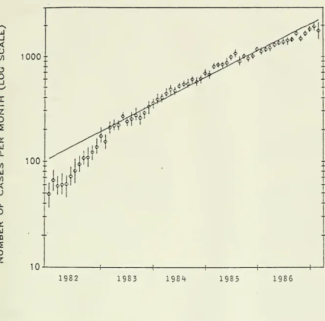
Figure 5 compares the non-parametric model of AIDS incidence to a

strictly exponential model. In contrast to earlier figures, the ordinate has

a logarithmic scale. The individual data points reflect the non-parametric

estimates, along with their approximate 95% confidence intervals. The fitted exponential model has an estimated slope of 0.0492, which means a doubling

u

_J

<

U

\n

o

O

_j

I

Z

q: Q. 00

u

<

u

Ll

o

tr

u

m

D

Z

1000

100-1982 1983

1984

1985

1986

FIGURE 5. _{Estimated Incidence Under} a Non-Parametric Model and an

Exponential Model of the AIDS Epidemic. (The incidence data are plotted

on a logarithmic scale. Approximate 95 percent confidence intervals are given for the _{non-parametric estimates.)}

-15-Under the exponential model, the estimated tails of the reporting delay

distributions were: S(63) = 0.331; S* (48) = _0; S" (12) = 0.215; and

£"'(7) = 0.328. An exponential model would thus require 33.1 percent

underreporting of AIDS cases during January 1982-March 1983 (interval 1) .

After August 1986 (interval 4) , the proportion of reporting delays in excess

of 6 months would be 32.8 percent. For the four intervals, the estimated proportion of cases reported in the same or the subsequent month (that is,

tt(0)+TT(1) ) were respectively: 0.330, 0.362, 0.337, and 0.267.

In all models analyzed, the duration of reporting delays was found to be

increasing over the course of the epidemic, especially after August 1986 (interval 4). If we convert ft, ft', ft" and ft"' into continuous

distibutions by linear interpolation, then in the non-parametric case, the

estimated median reporting delays (in months) would be, respectively: 1.10

(95% confidence interval 0.92 to 1.49); 1.79 (95% conf. int. 1.72 to 1.91);

1.73 (95% conf. int. 1.64 to 1.84); and 2.33 (95%% conf. int. 2.20 to 2.53).

5. CONCLUSIONS

By March 31, 1987, the CDC had reported 79 percent of all AIDS cases

diagnosed by that date. This divergence between reported and incident cases grew larger as the epidemic progressed (Figure 4) . If we projected the smoothed incidence model exp [p~o + Pit + ^>zt2 + (ht3

] out of sample, and if we

assumed that the reporting delay distribution ft'" remained unchanged,

then by December 31, 1990, only 285,000 (74 percent) of a cumulative total of

383,000 cases would be reported. While projections based upon purely

-16-1986), there are compelling epidemiological reasons to expect the incidence of

AIDS to continue to rise for at least the next five years (Brookmeyer and Gail

1986; May and Anderson 1987; Rees 1987; Harris 1987). Accordingly, the

difference between reported and diagnosed cases is likely to grow larger. I tentatively conclude that the distribution n has been shifting to the right. Since September 1986, about 70 percent of cases remain unreported two or months after diagnosis. This increase in the duration of reporting delays

has occurred in spite of (or perhaps as a result of) the partial automation of

the case surveillance system. I found the same trend toward increasing

reporting delays in separate analyses of AIDS cases in homosexual and bisexual men and in intravenous drug users. The same conclusion applied to separate analyses of AIDS cases first presenting with Pneumocystis carinii pneumonia,

with Kaposi's sarcoma, and with other conditions. In fact, the changing mix

of AIDS cases appears to go against the trend in reporting delays. Cases with Kaposi's sarcoma took significantly longer to report, with 78 percent now going unreported two or more months after diagnosis. Yet they comprise a

declining fraction of newly diagnosed cases (from 28 percent of cases

diagnosed in the first quarter of 1982 to 14 percent in the first quarter of

1987).

The CDC encoded the dates of diagnosis and case report by calendar month. Accordingly, I modeled the reporting delay phenomenon in discrete time. It is

unlikely, however, that a continuous-time model would have yielded markedly

different conclusions. In particular, in a continuous-time exponential

epidemic with a _{stationary reporting delay distribution, the discrete}

-17-with stationary reporting delays, n(0) would fall. Yet we observed n(0)

increasing.

There are two untested explanations for the trend toward longer delays. First, doctors and hospitals are taking longer to report cases to the health departments. Second, the health departments are taking longer to send the

reports to the CDC. While the latter explanation cannot be excluded from the

data at hand, the former deserves our serious attention.

Perhaps increasing case loads have overburdened treating physicians. In the early years of the epidemic, doctors may have had more incentive to report

a novel disease. Initially, infectious disease specialists made the diagnosis

of AIDS. Now, a different type of physician may be the first contact with an

AIDS patient. Successive changes in the official definition of AIDS may have created increasing confusion about which patients were to be reported.

In the non-parametric model, I found the doubling time of the epidemic to

have increased from about 6 months in 1982 to 15-16 months in 1986. As Figure

5 suggests, most of the deceleration occurred in 1982. If there was substantial underreporting during that period, the epidemic may not have

decelerated as much as it appears. Still, the conclusion that the epidemic is

decelerating to some degree appears reasonably robust.

REFERENCES

BROOKMEYER, R. and GAIL, M.H. (1986), "Minimum Size of the Acquired

Immunodeficiency Syndrome (AIDS) Epidemic in the United States," Lancet,

-18-CENTERS FOR DISEASE CONTROL (1986a), "Revision of the Case Definition of

Acquired Immunodeficiency Syndrome for National Reporting-- United States," Morbidity and Mortality Weekly Report , 34, 721-726, 731-732.

CENTERS FOR DISEASE CONTROL (1986b) , "CDC Classification System for HIV

Infections," Morbidity and Mortality Weekly Report, 35, 334-339. CHAMBERLAND, M.E., ALLEN, J.R., and MONROE, J.M. (1985), "Acquired

Immunodeficiency Syndrome, New York City: Evaluation of an Active

Surveillance System," Journal of the American Medical Association, 254, 383-387.

COX, D.R. (1975), "Partial Likelihood," Biometrika, 62, 269-276.

CURRAN, J.W., MORGAN, V.M., HARDY, A.M., JAFFE, H.W., DARROW, V.W., and

DOVDLE, V.R. (1985), "The Epidemiology of AIDS: Current Status and Future Prospects," Science, 229, 1352-1357.

DEMSTER, A.M., LAIRD, N.M. , and RUBIN, D.B. (1977), "Maximum Likelihood from Incomplete Data via the EM Algorithm," Journal of the Royal Statistical Society, Series B, 39, 1-22.

EFRON, B. (1979), "Bootstrap Methods: Another Look at the Jackknife," Annals

of Statistics, 7, 1-26.

HARRIS, J.E. (1987), "The AIDS Epidemic: Looking into the 1990s," Technology

Review, in press.

MAY, R.M. and ANDERSON, R.M. (1987), "Transmission Dynamics of HIV Infection," Nature, 326, 137-142.

MORGAN, V.M. and CURRAN, J.V. (1986), "Acquired Immunodeficiency Syndrome: Current and Future Trends," Public Health Reports, 101, 459-465.

REES, M. (1987), "The Sombre View of AIDS," Nature, 326, 343-345.

Date

Due

MIT LIBRARIES

3

^O&Q 005 lHI

™