Design and qualification of an absolute thickness measuring machine

Design and Qualification of an Absolute Thickness Measuring Machine by

Darcy K. Kelly

B.S. Mechanical Engineering

Massachusetts Institute of Technology, 2003 Submitted to the Department of Mechanical

Engineering in Partial Fulfillment of the Requirements for the Degree of Master of Science in Mechanical Engineering

at the

Massachusetts Institute of Technology June 2004

© 2004 Darcy K. Kelly All rights reserved

The author hereby grants to MIT permission to reproduce and to

distribute publicly paper and electronic copies of this thesis document in whole or in part.

Signature of A uthor... ... ...

Department of 1 hanical Engi ering May 7, 2004

Certified by... - - . .. . . . . Samir Nayfeh Assistant Professor of Mechanical Engineering Thesis Supervisor

A ccepted by ...

1 W, Ain A. Sonin

Chairman, Department Committee on Graduate Students

MASSACHUSETTS INSTMTiE OF TECHNOLOGY

Design and Qualification of an Absolute Thickness Measuring Machine by

Darcy K. Kelly

Submitted to the Department of Mechanical Engineering On May 7, 2004 in Partial Fulfillment of the Requirements for the Degree of Masters of Science in

Mechanical Engineering

ABSTRACT

The target fabrication group at Lawrence Livermore National Laboratory develops various high energy density physics targets, which are used to study the interaction of materials when shot with high energy lasers. These targets consist of many different types of materials glued together including low density foams, plastics, and metals. To verify models, the physicists need to know the exact thickness of the targets and target components to ± 1.0 pm. The target components are typically 3-5 mm in diameter and 200-300 pm thick and may have features such as moguls or two-dimensional sine waves machined onto them. As of yet, no commercial thickness measuring machine exists on the market capable of measuring thicknesses to ± 1.0 tm. To solve this problem, an absolute thickness measuring machine was developed that uses a precision air-bearing XY stage to scan a target between two confocal displacement lasers that measure the profile of each side of the target. A NIST traceable gage block of known thickness is used to calculate the thickness of the target.

This paper describes the design and qualification of the absolute thickness measuring machine. It focuses on the error budget and tests performed to qualify the machine. Without compensation factors, the absolute thickness measuring machine was able to measure the thickness of a gage block to 0.5 pm.

Thesis Advisor: Samir Nayfeh

Acknowledgements

I would like to thank all of the people at Lawrence Livermore National Laboratory for their technical advice and help, but also for their encouragement, and guidance about graduate school, working, goals, and my future.

A special thanks to Robin Hibbard for teaching me the difference between being a student and an engineer. Fluids research, especially in respect to water skiing, was a key lesson in learning that you must always make time for fun. I would also like to thank his family for including me in many of their family events when my family and friends were so far away.

The two Matts! Matt Bono and Matt Panzer, thank you for all your brainstorming sessions and for letting me distract you as much as possible. The two of you made working in a windowless sheet metal hell of a building a bit more bearable.

Thank you Hedley Louis, for bringing me to LLNL, and guiding me over the last three summers. Thank you Sam Thompson, Jeremy Kroll, and Carl Chung for teaching me the art of using straight edges, cap probes, and interferometers. Also thank you for being patient with my constant questioning about qualification tests.

Thank you Mike Wilson and Andi Nikitin for bailing me out several times when I got in a jam, and for your overall help in ensuring that I finished in time to go back to school in January. Thank you Jack Reynolds for being the only person I've ever met that

completes things on time. Why are there aren't more people like you?

A special thanks to all the machinists for cake, coffee, smiles, help, great conversations, and friendly baseball banter. Go Red Sox.

Thank you Walter Nederbragt for allowing me to live in your house, eating Twisters with me, going to the gym with me, and being a great friend. I miss our late night

conversations.

Thank you Stacia Swanson for helping me to edit my thesis, and for just being plain awesome. You are my hero!

Thank you Jodi Beggs for bubble tea, Dennis Gregorovic for Trivial Pursuit, Mike Bonnett for hugs, Todd Nightingale for yummy food, Rich Hanna for wine, Anne Dreyer

for being girly, Kevin Schmidt for laughter, Evencio Rosales for being smelly, Chris Cassa for "thesis writing work days," Doug Creager for green monster tickets, Sara Pierce for providing a knowing smile, the MIT softball team for many laughs, many

tears, and a lot of singing, and John Jannotti for constantly questioning how many pages I've completed, and for teaching me many things.

A special thanks to Samir Nayfeh for his help in writing this thesis and for signing it!!! A final thanks to my family for all of their encouragement and support over the last 5 years, and the many years before that.

Contents

1 Introduction... 9

2 Design ... 12

2.1 Conceptual D esign... 12

2.2 M easuring Procedure ... 13

2.2.1 Initial Laser A lignm ent ... 14

2.2.2 Z Stage M ovem ents ... 15

2.2.3 Perpendicular A lignm ent M ethod... 15

2.2.4 Collinear A lignm ent M ethod ... 16

2.3 Final D esign... 17

3 Analysis of Final D esign... 23

3.1 XY Stage M ovem ent (G eom etric) Errors... 27

3.2 Laser Errors... 30

3.3 Z Stage M ovem ent (Geom etric) Errors ... 32

3.4 Laser M isalignm ent ... 34

3.5 Therm al Expansion Errors... 37

3.6 V ibration Errors ... 38

3.7 Final Error Budget ... 38

4 Qualification Tests and Results ... 41

4.1 Straightness Qualification Tests ... 41

4.2 X Y Squareness... 48

4.3 Linear D isplacem ent Qualification Tests... 49

4.4 A ngular (Pitch, Y aw) Qualification Tests ... 53

4.5 A ngular Roll Qualification Test... 57

4.6 Z A xis Qualification Tests... 59

4.7 Laser Linear D isplacem ent Qualification Tests... 59

4.8 Updated Qualification Test and Compensation Factor Error Budgets ... 63

5 Conclusion ... 66 References... 68 Appendix A ... 69 Appendix B ... 71 Appendix C ... 73 Appendix D ... 77

List of Figures

Figure 1-1 Typical laser targets for high energy density physics experiments... 10

Figure 2-1 Conceptual diagram of the absolute thickness measuring machine... 12

Figure 2-2 Thickness calibration procedure. ... 14

Figure 2-3 Illustration of cosine error... 15

Figure 2-4 Collinear alignment of lasers. ... 17

Figure 2-5 Final model of the absolute thickness measuring machine... 18

Figure 2-6 The absolute thickness measuring machine. ... 19

Figure 2-7 Top and bottom Keyence lasers... 20

Figure 2-8 Laser flexure... 21

Figure 2-9 Target, gage block, and microscope slide fixture. ... 22

Figure 3-1 R otational errors... 24

Figure 3-2 Thickness error caused by an XY error... 26

Figure 3-3 Worst case scenario target... 26

Figure 3-4 Pitch, yaw, and roll for the X and Y axis of travel... 27

Figure 3-5 Straightness error ... 29

Figure 3-6 Keyence LT-81 10 confocal laser ... 30

Figure 3-7 Keyence LC-2420 triangulation laser. ... 31

Figure 3-8 Front and side view of the Z stage and laser... 34

Figure 3-9 Laser misalignment ... 35

Figure 3-10 Sketch of the displacement error from laser collinear misalignment... 36

Figure 3-11 Laser misalignment... 37

Figure 4-1 Normal straightness test and straightness reversal test setup... 42

Figure 4-2 Normal straightness test and straightness test reversal models... 43

Figure 4-3 X axis horizontal straightness. ... 44

Figure 4-4 Y axis horizontal straightness. ... 44

Figure 4-5 Straight edge straightness... 45

Figure 4-6 Setup for X axis vertical straightness test. ... 47

Figure 4-7 The X axis vertical straightness ... 47

Figure 4-8 The Y axis absolute vertical straightness... 48

Figure 4-9 Linear displacement test for the Y axis... 50

Figure 4-10 Michelson Interferometer... 51

Figure 4-11 The X axis linear displacement error ... 52

Figure 4-12 The Y axis linear displacement error. ... 52

Figure 4-13 Michelson interferometer measuring angular yaw error... 53

Figure 4-14 Setup for Y axis angular yaw test. ... 54

Figure 4-15 Setup for Y axis angular pitch test... 54

Figure 4-16 X axis pitch. ... 55

Figure 4-17 Y axis pitch. ... 55

Figure 4-18 X axis yaw ... 56

Figure 4-20 Setup for Y axis angular roll test... Figure 4-21 X axis roll... Figure 4-22 Y axis roll...

Figure 4-23 Setup for laser linear displacement test using the Clevite brush... Figure 4-24 Bottom confocal laser linear displacem ent. ... Figure 4-25 Top confocal laser linear displacem ent error... Figure 4-26 Bottom triangulation laser linear displacement error... Figure 4-27 Top triangulation laser linear displacem ent error. ... Figure B-I Top and bottom laser m ounting... Figure C- 1 Z axis yaw test setup... Figure C-2 Z axis yaw ... Figure C-3 Z axis pitch. ... Figure C-4 Z axis linear displacem ent error. ... Figure D -1 X axis horizontal straightness. ...

Figure D-2 Y axis horizontal straightness. ... Figure D-3 X axis vertical straightness... Figure D-4 Y axis vertical straightness... Figure D-5 X axis linear displacem ent. ... Figure D-6 Y axis linear displacem ent. ... Figure D-7 Z axis linear displacem ent... Figure D-8 X axis pitch... Figure D -9 Y axis pitch... Figure D -10 Z axis pitch... Figure D- 1 X Axis Yaw ... Figure D-12 Y axis yaw ... Figure D-13 Z axis yaw . ... Figure D-14 X axis roll... Figure D-15 Y axis roll...

57 58 58 59 60 61 62 62 71 73 74 75 76 77 78 78 79 79 80 80 81 81 82 82 83 83 84 84

List of Tables

Table 3.1 Error budget using manufacturer's specifications for a 3 mm diameter target. ... 4 0 Table 4.1 Error budget using qualification test results for a 3 mm diameter target. ... 64 Table 4.2 Error budget using qualification test results with estimated compensation

factors for a 3 mm diameter target... 65

Chapter 1

Introduction

Lawrence Livermore National Laboratory (LLNL) manufactures laser targets for high energy density physics experiments. These targets are generally smaller than 2 mm in size and are planar, cylindrical, or spherical. They consist of components and features that range in size from a few microns to a few hundred microns. Figure 1-1 shows a typical target manufactured at LLNL. Many of the components are machined to micron flatness and parallelism specifications, or in other cases have complex patterns machined into them. For example, a two-dimensional sine wave pattern (k=50 pm, A=5 ptm) might be machined onto the surface of a plastic disk. The patterns machined on the target surfaces have micron tolerance specifications and quantitative verification of these specifications is critical. One of the most important specifications is the absolute thickness of each component. The physicists performing these experiments must know the absolute thickness of the components for their experimental analysis and models. Most experiments involve shooting a target with a large laser and studying how the materials interact. The analyses are time-based, and require knowledge of the absolute thickness of the different target components to ± 1.0 pm, and sometimes to ± 0.1 pm, as well as knowledge of the shape of the target, or profile. Therefore, there is a need for a tool that measures both the component's thickness and surface feature profile to be

Gold support washer

Aluminum _Coppe

substrate _{sample Quartz windows}

Figure 1-1 Typical laser targets for high energy density physics experiments. On the left is a Equation of State (EOS) target, consisting of several components. On the right is a mogul surface target.

In many cases, because of the size, thickness, feature size, material, and surface finish of the target, the use of a contact probe for measurement is not acceptable. For example, often targets consist of components made from low density foams, known as aerogels. A contact probe tip would damage the surface of an aerogel target, ruining the target and altering the target after measurement. While several non-contact and contact

profilometers already exist, there is no commercial product available that will measure both the surface profile and thickness of a target to the physicists' specifications.

This paper will present the design, assembly, activation, and qualification of the thickness measuring tool. The main focus of the thesis will be to understand the sources of error in the design, including laser linear displacement and alignment, stage motion, and other significant errors such as thermal expansion and vibration. The results of the

qualification tests will be used to find the magnitude of these errors and to determine the overall accuracy of the machine. An error budget has been developed to identify the effects the errors described above have on the thickness measurement of the machine. It is presented in Chapter 3. The validation of these errors will be undertaken during qualification of the tool, which is presented in Chapter 4. To date, the machine has been able to measure a gage block of known thickness accurately to within 0.5 pm. Future

work necessary to verify this measurement and to improve the overall accuracy of the machine is presented in Chapter 5.

Chapter 2

Design

2.1 Conceptual Design

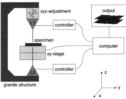
The conceptual layout for a non-contact absolute thickness measuring machine consists of two displacement lasers mounted collinearly and facing one another. The target is mounted on a fixture between the two lasers. The fixture is connected to an XY linear stage that provides the scanning motion of the part while the lasers remain fixed in place. The top laser is adjustable in the Z direction allowing for different height targets. The conceptual layout of the machine can be seen in Figure 2-1 below.

xyz-adjustment output controllerlo specimen computer xy-stage V1oILIol lerz granite structure

Figure 2-1 Conceptual diagram of the absolute thickness measuring machine.

Linear position data from the XY stage and target profile height data in the Z direction from each laser are output to the computer. This data will provide a top profile (x, y, zi) and bottom profile (x, y, Z2) of the target. The thickness data of the target (x, y, t) is

calibrated using a gage block of known thickness, H, that is scanned before and after each target measurement. The gage block measurement, and gage block thickness, H, are used to calibrate how far apart the top and bottom lasers are. Once this is determined, the profile data of the target is analyzed to find the absolute thickness of the target as a function of X and Y.

2.2

Measuring Procedure

The general procedure for measuring a target is listed below. Step 5 is optional but recommended.

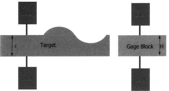
1. Focus each laser on the target surface (top and bottom) so that each laser will remain within its measuring range (± 300 pm) for the entire scan.

2. Move the XY stage so that the lasers are positioned above the gage block of known thickness, H. It is important to note that the thickness difference between the target and the gage block must be within the laser's measuring range, or the top laser will not be able to focus on the gage block without moving it in the Z

direction.

3. Calibrate the lasers. To do this, scan the gage block and use the profile data and the known gage block thickness to calculate the thickness calibration factor. See Appendix A for more details.

4. Reposition the lasers above the target and scan to get a measurement of the top and bottom profile of the target and a calculated absolute thickness.

5. (Optional) Scan the gage block again to verify the thickness calibration factor. This will also help determine how much thermal drift occurred during the measurements.

I

I

_I

Figure 2-2 Thickness calibration procedure. A gage block of known thickness, H, is scanned before and after the target is measured to calibrate the thickness of the target, t.

2.2.1 Initial Laser Alignment

For accurate measurements and to minimize errors, the lasers need to be aligned collinearly to within 0.5 pm in X and Y, and to .04* angularly. These numbers were determined geometrically by estimating the best possible alignment that could be

achieved with current alignment techniques (described in Sections 2.2.3 and 2.2.4). This means that the lasers need to be adjustable in X, Y, Z, 0X, and Oy. It is also important that the lasers are aligned perpendicular to the target to prevent the occurrence of cosine errors.

A cosine error is best described by looking at Figure 2-3 below. If a laser is aligned perpendicular to the target, it has a correct measurement of length Z. However, if it is tilted an angle, 0, away from perpendicular then it will measure a different length, Z', and therefore will have a cosine measurement error. The cosine measurement error, 8z, is given by

0

z

Figure 2-3 Illustration of cosine error.

To align the lasers, the top laser is first aligned perpendicular to the target. Next, the bottom laser is aligned in X and Y to the top laser, and finally in Ox and

Qy.

2.2.2 Z Stage Movements

It is important to note that every time the top laser is moved in the Z direction, the lasers will become misaligned due to pitch, yaw, roll, and straightness errors in the Z stage. Therefore, it is desirable to have a way to verify the alignment of the lasers before each measurement. Although the Z stage cross roller bearings are highly repeatable, the Z stage should never be moved during a measurement or thickness calibration unless it is absolutely necessary. An alignment procedure must be developed to align the lasers when they are more than 5.6 mm apart. The current alignment method described below only works when the lasers are less than 5.6 mm apart.

2.2.3 Perpendicular Alignment Method

To align the top confocal laser perpendicular to the target, adjust the angle of the lasers in both

Ox,

A method to align the triangulation lasers perpendicular to the target still needs to be developed. This thesis focuses primarily on the alignment of the confocal lasers.

2.2.4

Collinear Alignment Method

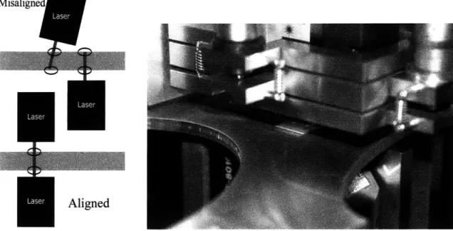
To align the lasers collinearly, a transparent microscope slide of height, hslide, is used. The microscope slide is placed between the lasers resting on the fixture as shown in Figure 2-4. The operator looks at the laser spots diffracted on the top and bottom

surfaces of the microscope slide by looking through a microscope mounted on the side of the machine. If the lasers are not collinearly aligned, four spots will show up on the slide (two spots for each laser). The reason that there are two spots for each laser is the laser is hitting the top and bottom surface of the slide, so there will be a spot on the top and bottom of the slide for each laser. If the lasers are aligned collinearly, then there will only be two spots (one on top and one on the bottom) because the laser beams will be overlapping. The collinear alignment error is a function of the XY resolution of the lasers, human error, and the thickness of the slide (hslide). The human error and XY resolution error may be able to be decreased by using a colored filter to make one laser a different color. This will allow the operator to better differentiate between the two lasers,

*~ I~1'1~ -

-Figure 2-4 Collinear alignment of lasers. If the lasers are misaligned the operator will see 4 spots (pictured upper left, and to the right). If the lasers are aligned collinearly, the operator will see 2 spots (lower left).

An alternate method for aligning the confocal lasers is to have the lasers look directly at each other. If there is no object between the two lasers, each laser will try to read the laser signal from the opposing laser. Each laser has a CCD camera in it that is connected to a monitor. The operator is able to see opposing laser beam on the monitor. The monitor also has a target that shows where the beam center should be. The operator can then use the cameras to align the lasers collinearly with one another, but centering them in the target on the monitor. This alignment technique is not validated yet, because it is unknown how well the cameras are aligned with the laser beam and the target on the monitor.

2.3 Final Design

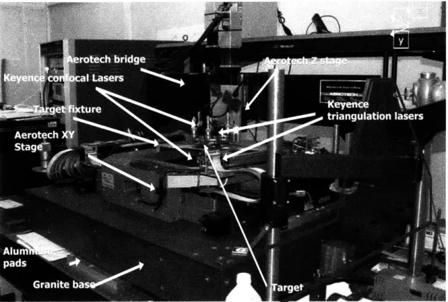
The final design consists of an Aerotech linear air-bearing XY stage (ABL3600-250-250) sitting on a large four-foot by four-foot granite base [2]. The granite base is bolted to a Newport RS 4000 optical table that is supported by four Newport pneumatic XL-G legs [6]. Connected to the sides of the XY stage is an aluminum bridge also made by

.1, 1- ;b 96 - - t - § - - - _ - - - -. -, _ _

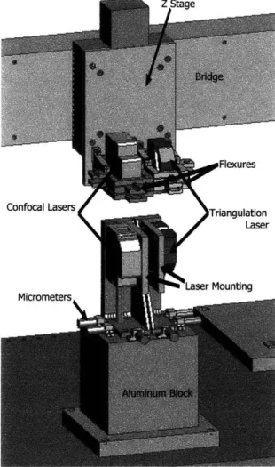
roller bearing linear Z stage (ATS 15010) centered over the XY stage [1]. Attached to the Z stage are two flexures that hold two different types of non-contact linear displacement lasers made by Keyence: a confocal laser (LT-8010), and a triangulation laser (LC-2420) [5]. The XY stage has a hole in the middle allowing for another confocal laser (LT-8010) and triangulation laser (LC-2420) to shine upwards and measure the bottom of the target. A CAD model of the final design is pictured in Figure 2-5 and a picture of the final machine is shown in Figure 2-6.

Aerotech bridge Keyence confocal Lasers

Target fixture

-1~~~ - -~

Figure 2-6 The absolute thickness measuring machine.

The LT-8010 confocal displacement laser has a resolution of 0.1 pm, and a measuring range of 300 pm. It can measure both diffuse and specular surfaces. It can also measure the thickness of a translucent material as long as the thickness is within the laser's measuring range. This property of the confocal laser is especially important for target fabrication because it allows the operator to measure the profile and thickness of a bond (such as an epoxy) holding two translucent materials together. The machine can also be adapted to hold an LT-8 110 confocal displacement laser with a measuring range of 1 mm, and a resolution of 0.2 pm. The LT-81 10 laser has a larger working distance than the LT-8010 (10 mm instead of 5 mm), which could become important in the future for measuring larger parts at the lab, when a larger clearance area is needed (as in a part with a large step height) [5].

The LC-2420 triangulation displacement laser has a resolution of 0.01 Im, and a measuring range of± 200 im. The LC-2420 laser is only able to measure highly

reflective or mirror like surface targets. The triangulation laser will be used to measure component's thickness that needs to be known to better than ± 0.1 Pm accuracy.

The majority of this thesis will focus on using the confocal laser (LT-80 10) rather than the triangulation laser (LC-2420) to measure targets because of its wider range of measurement capabilities. Both lasers will be discussed further in Section 3.2.

Confocal Lasers

Triangulation_Laser

Figure 2-7 Top and bottom Keyence lasers.

The Aerotech XY stage has a 16 inch by 19 inch rectangular hole. The granite base which it is mounted on also has a hole approximately 16 inches by 8 inches through it. Two other Keyence lasers (LT-8010 and LC-2420A) are mounted in this hole pointing upwards in order to measure the bottom surface of a target. The Aerotech XY stage has

____________________________________ - -- - - - - -- iitv -

-250 mm of travel in both the X and Y axis. This allows the machine to measure a target

as large as 250 mm by 250 mm by 100 mm. Furthermore, targets of almost any surface can be measured because of the two different lasers available for measurement.

The bottom lasers are adjusted in the X and Y directions to ± 0.5 mm using three

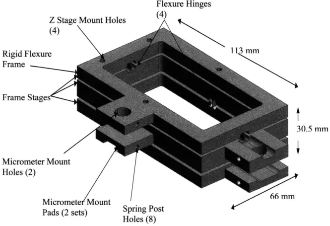
micrometers. They can also be adjusted angularly in Ox, and Oy by 0.013 radians (.76 degrees) using micrometers. The top lasers can be adjusted in Ox, and 0y with a range 0.026 radians (1.5 degrees) by using the flexure in Figure 2-8 below.

Z Stage Mount Holes (4) Rigid Flexure Frame Frame Stages Micromete Holes (2) r Mount Micromete Mount Pads (2 sets) Flexure Hinges (4) A 66mm Spring Post Holes (8)

Figure 2-8 Laser flexure. The laser flexure allows the top laser to be adjusted in Ox and Oy.

The target being measured, the gage blocks used for thickness calibration, and the microscope slide used for laser alignment are placed on the fixture shown in Figure 2-9, which spans the length of the hole in the XY stage. This fixture can be raised higher to allow for the LT-81 10, which is taller than the LT-8010. The fixture is 6 mm thick, allowing for a 2 mm clearance above and below for the lasers.

t

Chapter 3

Error Budget

An error budget was made in order to estimate the accuracy of the machine. An error budget specifies the amount of error allowed for each component on the machine, or, in this case, estimates how much error each component will contribute to the system. For every machine there are errors in all six degrees of freedom, and each machine

component can contribute differently to these errors. Rather than use the HMT method (Homogeneous Transformation Matrices) described by Slocum [7], the error budget here is simplified by estimating the total error for a standard size target of diameter D. To find the overall accuracy of the machine the root mean square of the errors was calculated. The error budget in this thesis uses the peak-to-valley amplitude error (maximum error-minimum error) for each component. Although some of these errors are systematic errors

(repeatable errors), because the error budget treats the errors as if they were random by using the peak-to-valley amplitude of each error, the best estimate of the total error is

calculated by taking the root mean square of the components rather than the sum [7].

For each axis there are three translational displacement errors (6x, 8y, dz), and three rotational errors (ex, Fy, Cz). The main types of errors in the system are geometric errors, sensor errors, alignment errors, thermal errors, and vibration errors.

For profile measurements the most important errors are the displacement errors, especially the Z direction errors, or height errors. For that reason, the rotational errors acting over the target diameter are converted into displacement errors in this error budget. The rotational errors create Abbe errors, otherwise known as sine errors [7]. This is because the error acts over a lever arm -in this case the diameter of the target, D. The sine errors and cosine errors for each rotational error are described below. Abbe errors

r~r --

--(sine errors) are the most important to pay attention to, as they are much larger than cosine errors.

The Abbe error, 8,, in Figure 3-1 below is

S5, = D sin 0 (3.1)

and the cosine error, 6, is

8, = D - D'= D(1 - cos 0) (3.2)

If the cosine error is large it can greatly effect the target measurement, because instead of the lasers measuring a point on the target, X, it would be measuring point, X' that is 8x

away from X. If the target had a mogul surface as seen in Figure 1-1, then it would have the wrong measurement for point X.

D

6z

II

Figure 3-1 Rotational errors. The sine error is the Abbe error. There is also a cosine error.

Equations 3.3 though 3.8 describe the displacement errors for each axis caused by cosine and sine errors. Notice that each rotation causes a variety of errors, demonstrating the need to organize these errors neatly in an error budget.

As seen above, the rotational error about the Y axis creates a cosine error, 6x, in the X direction

8 , = D( - cos) (33

and a sine error, 6,, in the Z direction

o, = D sin 9, (3.4)

Similarly, the rotational error about the X axis creates a cosine displacement error, 6y, in the Y direction

8, = D(1 - cos 9) (3.5)

and a sine error, 6z, in the Z direction

c,5 = D sin ., (3.6)

A rotation about the Z axis causes a cosine error, 8x, in the X direction

, = D(1- cos0.) (3.7)

and a sine error, 8y, in the Y direction

S, = D sin 0, (3.8)

For absolute thickness measurements, there are thickness displacement errors, and displacement errors in the X and Y directions. Again, in this error budget, the rotational errors are converted into displacement errors as described above. It is important to note that any error in the X and Y directions creates a thickness error, as seen in the diagram below. If a target is not perfectly flat then an error in X or Y will case the laser to measure the wrong thickness for that specific XY position (Figure 3-2).

LJ~ -. - -

-Where thexy

I

stage thinks it is

I

ii

_position

stage actual

Figure 3-2 Thickness error caused by an X-axis displacement error.

Therefore, the thickness error, 6t, due to 8x and 6x is

, = 21,52 +52 tan0, (3.9)

where O, is the angle of a feature on both sides of a target. For target fabrication at LLNL, it is assumed that worst case scenario is when a target has a feature on both sides with a 100 angle as drawn in Figure 3-3 below.

100

h

All geometric displacement errors in the Z direction cancel out for absolute thickness measurement. For example, the error caused by the XY stage pitching will be measured by both the top and bottom laser, and therefore will not enter into the absolute thickness measurement, since the two terms will cancel each other out. However, non-geometric errors in the Z direction, such as laser linear displacement, will not cancel each other out. This will be discussed further in Section 3.2 below.

3.1 XY Stage Movement (Geometric) Errors

As the XY stage moves along the X axis, there is a linear displacement error in X, 6x(x), a horizontal straightness error in Y, 8y(x), and a vertical straightness error in Z, dz(x).

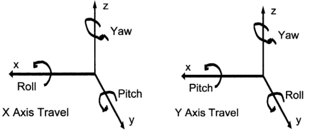
Similarly, there are three linear displacement errors as the XY stage moves along the Y axis: 6x (y), 6y (y), dz (y). The three rotational errors for the X axis are the pitch, ey (x), the yaw, sz (x), and the roll, ex (x). The rotational errors for the Y axis -pitch, F, (y), yaw, sz (y), and roll, ey (y) (roll) -can be directly translated into displacement errors as described above.

z _z

Yaw _{S Yaw}

Roll _{Pitch Pitch}

Roll

X Axis Travel Y Axis Travel

y y

Figure 3-4 Pitch, yaw, and roil for the X and Y axis of travel.

For a target of diameter D, the pitch for X axis travel causes a cosine error, 6x(x), in the X direction and a sine error, 6z(x), in the Z direction

,,(x) = D sin 0, (3.11)

The roll for the X axis travel causes a displacement error, 6y(x), in the Y direction, and a sine error, 6z(x), in the Z direction

5, (x) = D(I - cos Oj) (3.12)

9, (x) = D sin ., (3.13)

The yaw for X axis travel causes a cosine error, 6,(x), in the X direction and a sine error, 6y(x), in the Y direction, where

5, (x) = D(l - cos 9.) (3.14)

5,(x) = D sin , (3.15)

Similarly, we have the same equations for Y axis travel

(5, (y) = D(I - cos OY,) (3.16)

3,(y) = D sin 9, (3.17)

,(y) =D( - cos Ox) (3.18)

15, (y) = D sin Ox (3.19)

I - --- - -

-The two largest contributors to displacement error from the XY stage are horizontal and vertical straightness errors. A horizontal straightness error occurs when the XY stage is moving along one axis, but has a displacement error along the other axis. This is pictured in Figure 3-5 below. Vertical straightness has a displacement error in the Z direction as the axis travels in X or Y. For a thickness error, the vertical straightness error cancels out due to the collinearity of the lasers. In other words, a vertical stage movement will be measured by both lasers, and therefore won't be seen in the thickness measurement. Another XY stage geometric error that needs to be measured is the orthogonality of the X and Y axis.

Figure 3-5 Straightness error. Straightness error in the y-axis creates an error in the x direction for a mogul surface. The white line is ideal motion of the xy stage as it travels along the y axis. The gray line is the actual motion.

A horizontal straightness error, pictured above, can create a thickness measurement error because of an X or Y displacement error (see Figure 3-2). In Figure 3-5 above, the XY stage is not actually moving along the white line, but is really zigzagging along the grey line creating an X displacement error. Horizontal straightness error also creates a height error in a profile measurement for the same reason. The thickness error due to this displacement in X is calculated in Equation 3.7.

3.2 Laser Errors

To better understand the errors in the lasers, it is important to understand how they work. The LT-80 10 confocal laser measures the height of a sample by shining a laser diode down through a series of optics onto a target. The reflected light from the target then shines back up through the optics into a pinhole, where a sensor records the intensity. The key to the confocal microscope is that two of the optics are vibrating up and down as if they were attached to a tuning fork. The movement of these optical lenses changes the focal point of the laser. As the reflected light from the target shines back up through the optics, the intensity detector records the position of the vibrating optics when the

diffracted light is at its peak intensity. In other words, when the vibrating optics bring the laser into focus on the target surface, the light reflected back into the sensor is at its peak intensity [5]. The confocal laser is able to measure a variety of materials and surfaces because it uses the peak intensity of the reflected light to measure the height of a target, rather than just converting light intensity, which varies with material and surface properties, directly into a height measurement.

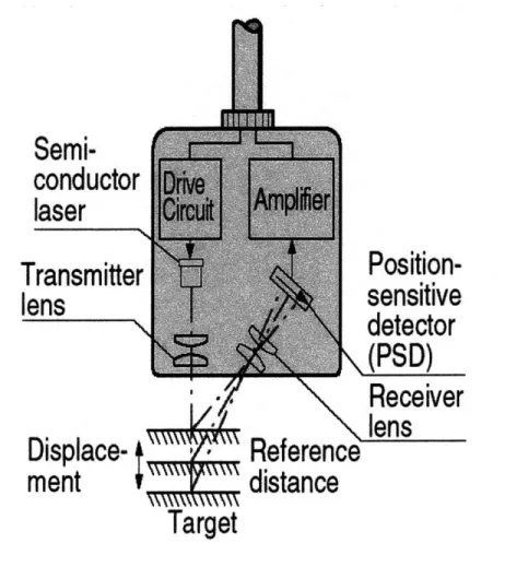
The LC-2420 triangulation laser is much simpler to understand. It simply bounces light off of a surface into a position sensitive detector. As the target height varies, the angle of the diffracted light reflecting into the sensor will also vary. A change in angle of the diffracted light will create a change in position on the position sensitive detector as seen in Figure 3-7 below. Therefore, the triangulation laser is able to convert a lateral movement on the position sensitive detector into a height measurement for a target.

Semi-conductor

laser

Position-Transmitter

Pesitive

lens

sensitive

detector

(PSD)

-f

Receiver

Displace-

Reference

ment

distance

Target

Figure 3-7 Keyence LC-2420 triangulation laser. Courtesy of Keyence Cooperation of America.

There are two important displacement laser specifications that cause measurement uncertainty: linear displacement and laser resolution. The largest error is the laser linear

displacement error. A linear displacement error occurs, for example, when the target is moved 50 ptm, but the laser outputs 51 pm, giving a 1 pm displacement error.

lasers is approximately ± 1.0 pm for the confocal laser and ± 0.4 pm for the triangulation laser, the linear displacement errors are repeatable to 0.4 Pm and 0.1 Pm respectively. This means that compensation factors can be calculated and inserted into the data file to make the machine more accurate.

The resolution of the laser is defined as the minimum separation at which one can tell that there are two objects rather than one. In this case, the resolution, p, of the confocal laser is taken to be

p = A/sina (3.22)

where A is the wavelength of the laser light (670 nm), and a is the aperture angle of the

optics (~45'). In this case, the lateral resolution of the confocal displacement laser is

approximately 1.0 pm (half the laser spot size diameter). The vertical resolution of the LT-8010 confocal laser is specified by the manufacturer to be 0.1 pm [5].

3.3 Z Stage Movement (Geometric) Errors

The Z stage movement errors are similar to the XY stage movement errors, except they only need to be taken into account if the Z stage is moved while measuring a target or between thickness calibrations. For the purposes of this thesis, it is assumed that the Z

stage will not be moved during measurement or thickness calibration, and therefore the errors will not be added into the error budget for the machine. The primary Z stage errors-- straightness, linear displacement, pitch, yaw, and roll -are described below, but not included in the actual error budget.

The pitch of the Z Stage, or rotation about the X axis creates a tangential error, 6y(z), in the Y direction and a cosine error, 6z(z), in the Z direction

where 1 is the distance between the center of the Z stage and the laser point in the Z direction and wd is the laser's working distance. A sketch of the laser position with respect to the Z stage can be seen in Figure 3-8.

The Z stage yaw, or rotational error about the Y axis, creates a tangential error, 6x(z), in the X direction and a cosine error, 6,(z), in the Z direction

5,(z) = 1 tan 0, (3.25)

, (z) = wd(cos 0, -1) (3.26)

The Z axis roll produces an X and Y displacement

w(Z)

= VW2 + m2 (cos6-) (3.27)

8,(z)= w2 _+m2 _{sin, (3.28)}

where w is the distance from the center of the Z stage to laser measurement axis in the Y direction, and m is the distance from the center of the Z stage to the laser measurement axis in the X direction.

z Z Stage z ' y Z Stage Loser, rz cx m' dy

Figure 3-8 Front and side view of the Z stage and laser

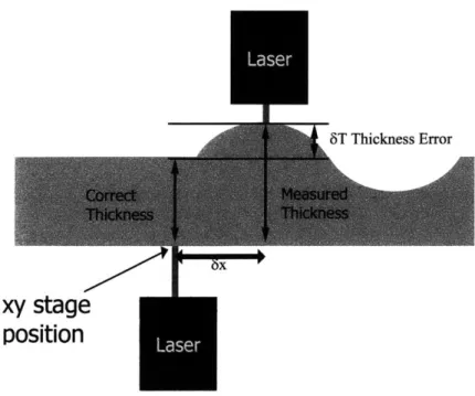
3.4 Laser Misalignment

Laser misalignment is one of the primary error sources for the absolute thickness measuring machine. The lasers must be aligned collinearly to one another and

perpendicularly to the target. Figure 3-9 below shows the thickness error that is created if the lasers aren't aligned in X and Y. In this case it is assumed that the lasers are

perpendicular to the target.

W

Laser

z wd

I

8T Thickness Error

xy stage

position

Figure 3-9 Laser misalignment in X creates an absolute thickness error, 8T.

It is assumed that the lasers can be aligned in the X and Y directions using the

microscope slide procedure described in Section 2.2.4 to half the spot size of the laser. The collinear misalignment of the lasers is then given by

0, = arctan(p/hslide)

9, = arctan(p/hslide)

(3.29)

(3.30)

where 0x and Oy are the angular misalignment of the lasers, p is half the spot size of the laser, and hslide is the height of the microscope slide.

This angular misalignment between the lasers creates displacement errors

(3.31)

(3.32) ;, = h tan(O,)

where h is distance between the two laser spots in the Z direction. It is important to remember that these laser displacement errors create a thickness error as seen in Figure 3-9 above. z Th x ~dx/ h/ h

Figure 3-10 Sketch of the displacement error from laser collinear misalignment

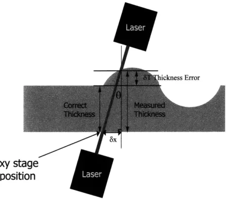
Thickness errors are also created if the lasers are aligned collinearly to each other, but not aligned perpendicular to the target. In Figure 3-11, the lasers are aligned collinearly, but not aligned perpendicular to the target, and are therefore measuring at different X

positions on the target. The X error between the two targets, 8x, creates an absolute thickness error, 6T.

5x

xy stage

position

Figure 3-11 Laser misalignment. If the lasers are aligned collinear, but not perpendicular to the target, there is a thickness error.

The X and Y displacements from perpendicularity misalignment between the target and the lasers are

&=h tan(,) (3.33)

3y =h tan(') (3.34)

where h is the distance between the two laser beams in the Z direction.

3.5

Thermal Expansion Errors

Errors due to thermal expansion for the system can vary depending on how long it takes to measure a target. Due to the fact that the bottom and top lasers are not on the exact same thermal loop, they will expand and contract at slightly different rates than each other. Taking the optical table as the starting position, the bottom laser is attached to

approximately 345 mm of aluminum blocks and plating. The top laser however, is attached to an aluminum plate, which is attached to the cross-roller bearing z-stage

(steel), which is attached to the aluminum bridge. The aluminum bridge is attached to the granite which in turn is attached to the optical table though three 25.4 mm aluminum plates. These different thermal loops can cause errors in the micrometer range if the room in which the absolute thickness measuring machine sits is not temperature

controlled. See Appendix B for a detailed thermal analysis.

3.6 Vibration Errors

Different vibrations in the room and vibrations from the motors on the XY stage may also cause errors in the system. Most of the vibrations in the room are negligible because the system sits on an isolated optical table. The largest vibrational errors in the system are due to vibrations from the XY stage linear motors or from the motor in the Z stage. These can also be neglected if a low pass filter is used to filter out any high frequency noise in the data caused by XY and Z stage vibrations.

3.7 Final Error Budget

The final error budget is shown in Table 3.1 below. Numerical errors for each source of error described above as specified by the manufacturer are shown. If the manufacturer's specification could not be found, the numbers were estimated or geometrically calculated to the best of the author's knowledge. The largest sources of errors are indicated in bold type. These are the errors that need to be verified with the qualification tests discussed in Chapter 4, and compensated for if possible. The total error for each axial direction is shown at the bottom of the table. This was calculated by taking the square root of the sum of the squares of the errors for each axis. Without compensation, there is 1.059 pm of error in the X direction, 1.049 ptm of error in the Y direction, and 2.312 pm of error in the Z direction for each laser. The thickness error for a flat target is 3.007 Pm, and for a featured target (pictured in Figure 3-3 above) is 3.050 ptm. These numbers can be further reduced with compensation factors. A corrected error budge is shown at the end of

manufacturer's specifications. An error budget using compensation factors is also presented at the end of Chapter 4. It shows a large improvement in machine accuracy

since the largest machine errors come from linear displacement errors that are highly repeatable and therefore can be mapped out and compensated for.

Table 3.1 Error budget using manufacturer's specifications for a 3 mm diameter target.

Type of Error

Featured Flat Part Part X Error Y Error Z Error Thickness Thickness

Component (s~m) (n) (sm) Error (sm) Error (prn)

Spot size 1.OOE+00 I.OOE+00 O.OOE+00 O.OOE+00 O.OOE+00

Resolution in z 1.OOE-01 2.OOE-01 2.OOE-01

Drift I.OOE-02 1.OOE-02 1.OOE-02 2.OOE-02 2.OOE-02

Linearity [_1.50E+00 3.OOE+00 3.OOE+00

Pitch (x axis) O.OOE+00 2.40E-08 6.OOE-03 6.OOE-1 I 8.52E-09

Pitch (y axis) 2.40E-08 O.OOE+00 6.OOE-03 6.OOE-1 1 8.52E-09

Yaw (x axis) 3.OOE-09 3.OOE-03 O.OOE+00 O.OOE+00 1.06E-03

Yaw (y axis) 3.OOE-09 3.OOE-03 O.OOE+00 O.OOE+00 1.06E-03

Roll (x axis) 1.60E-1 I O.OOE+00 4.OOE-06 O.OOE+00 5.64E-1 2

Roll (y axis) O.OOE+00 1.60E-1 1 4.OOE-06 O.OOE+00 5.64E-1 2

Vertical straightness Xz 8.97E-01 O.OOE+00 O.OOE+00

Vertical straightness Yz 2.05E-01 O.OOE+00 O.OOE+00

Horizontal straightness Xy 6.OOE-01 O.OOE+00 O.OOE+00 2.12E-01

Horizontal straightness Yx O.OOE+00 6.OOE-01 O.OOE+00 2.12E-01

Linearity (x axis) 7.46E-01 O.OOE+00 O.OOE+00 O.OOE+00 2.63E-01

Linearity (y axis) O.OOE+00 3.69E-01 O.OOE+00 O.OOE+00 1.30E-01

Zstage ____________

Pitch O.OOE+00 8.93E+00 1.02E-05 1.02E-05 3.15E+00

Yaw 2.51 E+00 O.OOE+00 8.1OE-07 8.1OE-07 8.86E-01

Roll 1.16E+00 1.16E+00 O.OOE+00 O.OOE+00 5.80E-01

Straightness Zx 2.OOE+00 7.05E-01

Straightness Zy 2.OOE+00 7.05E-O1

Linearity 3.93E+00 3.93E+00

Align top laser perpendicular 3.73E-01 7.33E-01 O.OOE+00 O.OOE+00 2.90E-01

Align lasers collinear (2 pt method) 2.50E-01 2.50E-01 O.OOE+00 O.OOE+00 O.OOE+00

Gage block height accuracy 1.OOE-02 1.OOE-02

Gage vs target height error 6.25E-02 6.25E-02 O.OOE+00 O.OOE+00 3.12E-02

Other

Thermal drift I 1.50E+00 I 2.OOE-01 I 2.OOE-01

M

Chapter 4

Qualification Tests and Results

4.1 Straightness Qualification Tests

The straightness error of an axis is the error in the direction perpendicular to the direction of travel as shown in Figure 3-5. To measure the straightness of the X axis, 6y(x), and the straightness of the Y axis, 8x(y), a fixed capacitance probe was used to measure the gap between itself and a precision straight edge. The straight edge was mounted on the XY stage, so that as the XY stage moved along an axis, the capacitance probe measured the gap as a function of X or Y. The capacitance probe is able to measure the gap between the probe tip and straight edge by converting the voltage from the change in

capacitance (dependent on gap size) into a length measurement. The data collected from the straightness test is both a measure of the straightness of the machine and the

straightness of the straight edge. Therefore, to obtain only the straightness of the machine, a reversal straightness test was performed. To do a reversal straightness test, the straight edge is simply rotated 1800, so that the cap probe measures the same part of the straight edge, but is facing in the opposite direction as seen in Figure 4-1 below. Following the initial test and reversal test, there are two sets of data and two unknowns, giving equations

N(x)= M(x) - S(x) (4.1)

R(x) = -M(x) - S(x) (4.2)

where N(x) is the first straightness test data, R(x) is the reversal test data, M(x) is the machine straightness, and S(x) is the straightness of the straight edge. The machine straightness is then

M(x) = [R(x) - N(x)] / 2 (4.3)

and the straightness of the straight edge is

S(x) = [R(x) + N(x)] 2 (4.4)

Figure 4-1 Normal straightness test and straightness reversal test setup.

The reason for straightness reversal is better understood by looking at Figure 4-2. This figure shows a semi-circular bump (straightness error) on the straight edge and a triangular bump (straightness error) on the XY stage. For the normal straightness qualification test (top of Figure 4-2) the capacitance probe measures the semi-circular bump in the straight edge and the triangular bump in the XY stage. The normal straightness measurement, N(X), is graphed on the right. For the reversal straightness qualification test (bottom of Figure 4-2) the capacitance probe again measures the semi-circular bump on the straight edge, but this time the triangular bump on the XY stage is in the opposite direction because the capacitance and probe and straight edge were rotated

180*. A plot of the reversal straightness, R(X), is seen on the right. By paying close attention to the sign convention of the straight edge and XY stage, it is easy to see how Equations 4.1 and 4.2 are derived.

Normal Straightness Test

X Travel

N(X)=-M(X)-S(X)

Reversal Straightness Test

X Travel

R(X)=M(X)-S(X)

Figure 4-2 Normal straightness test and straightness test reversal models.

The X axis horizontal straightness is shown below in Figure 4-3. Six dynamic test runs were performed along the X axis using a capacitance probe and straight edge as pictured above in Figure 4-1 for both the straightness test and the reversal test. The slope from the data was removed to account for initial straight edge misalignment for both sets of data. The six runs from each test were then averaged, and Equation 4.3 was used to find the X axis horizontal straightness. From the graph below, the absolute X axis horizontal straightness error is 0.15 pm. Appendix D shows plots for all six runs for each qualification test presented in this chapter.

0.0 0 -0.02 -0.04 -0.06 -0,08 -0A -0,12 -0.14 -0,16 50 100 150 Xaxis Position (mm) 200 250

Figure 4-3 X axis horizontal straightness. The absolute error in the Y direction as function of X is 0.15 gm.

The Y axis horizontal straightness is an error in the X direction as a function of Y. As seen in Figure 4-4 below, the absolute Y axis horizontal straightness error is 0.25 pim. Again, the graph below is calculated from Equation 4.3, and is averaged over six test

runs. 0.15 0.1 0.05 0 -0.05 -0.1 -0.15 -12

Y Axis Horizontal Straightness

--- --- + -- -- + --- ---

---0 50 100 150 200 250

Y Axis Position (mm)

Figure 4-4 Y axis horizontal straightness. The absolute error in the X direction as a function of Y is

0.25 sm.

E

X Axis Horizontal Straightness

--

--- --- --- --- - - - -I - - - -1

-0

From Equation 4.4, the straightness of the straight edge can also be found. Figure 4-5 below shows the plot of the straight edge straightness. The straight edge is straight to 0.91 pm over 200 mm. E 1-2 1 0.8 0.6 0.4 0-2 0 -0.2 0

Straigt Edge Straightnss

-- - --- - - - - -- - --- - -- - -- -I - -- - -- - -- -- - -- - -- --

--- -- - - -- - - -- - -

-50 100 160

Straight Edge Position (mm)

200 250

Figure 4-5 Straight edge straightness. The straight edge is straight to 0.91 pm over the 200 mm scanned.

The straight edge straightness found above can now be used to find the vertical straightness of the X and Y axis. The vertical straightness tests are similar to the horizontal straightness tests, except that the cap probe is measuring the straight edge in the Z-direction. The setup is shown in Figure 4-6. For vertical straightness, there is a third term in the equation caused by the effects of gravity on the straight edge. Thus equations 4.3 and 4.4 become

M(x) = [R(x)-N(x)]/2-t,(x)

S(x) = [R(x) + N(x)] / 2 - S, (x)

(4.5)

This gives two equations and three unknowns. To find the displacement in the straight edge caused by gravity, 8, (x), the displacement of the beam can be modeled using fundamental beam bending theory. A finite element model can be made, or the calculations can be done by hand. For this qualification test, the straight edge was modeled as a beam supported freely by two supports, so that the overall displacement was minimized (supports were placed 0.223*L away from the ends, where L is the length of the straight edge). The displacement of the beam between the two supports is given by

8 (x) = WX(IX)(l X)+l3 - 6C2) (4.7)

24EIL

where x is the distance from the support, W is the load per unit length, E is the modulus of elasticity, I is the moment of inertia of the beam, L is the total length of the beam, 1 is the length between the supports, and c is the distance from the edge of the beam to the support. The displacement of the beam between the edge and the support is then

Wu

0,(W)=

24EIL

where u is the distance from the edge of the beam to the support. Using Equation 4.3, 4.7, and 4.8, the average X axis vertical straightness is plotted below in Figure 4-7. It is seen that over a 200 mm span, the absolute error in the Z direction as a function of X is 0.40 [im. The Y axis vertical straightness is 0.51 pm over 200 mm of travel (Figure 4-8)

Figure 4-6 Setup for X axis vertical straightness test. E E 0.35 0.3 0.25 0.2 0.15 0.1 0.06 0 -0.05 -0.1 C 50 100 150 X Axis Position (mm) 200

Figure 4-7 The X axis vertical straightness absolute error is 0.40 gm.

---+ - - ---+ --- + -- -+--- - --- --- -- - --- ---- - --- --- --- - ----- --- - ---- --- --- --- --- --- --- --- --- --- -- -- -- -- -- --- - --- -- -- -- --- -- -- --- --- -- --- --- ---260

0 U) E 0 U E 0.2 01 0 401 -0.2 -0.3 -04 405

Y Axis Vertial Straightnes

-- -- --- -- -- - - --

-50 100 150

Y Axis Position (mm)

200 250

Figure 4-8 The Y axis absolute vertical straightness error is 0.51 jpm.

4.2 XY Squareness Qualification Tests

The squareness of the X and Y axes was found by measuring a square with a cap probe. Again, as in the straightness tests, a reversal test must be done to find the squareness of two axes. To find the squareness of the X and Y axes, regular straightness data was collected along the Y axis. Then, straightness data was taken along the X axis. For the reversal test, the square was flipped 180 degrees, and again the X and Y axis straightness data was taken.

The two tests give us the equations

01= a +

f8

02= a -i

(4.9)

(4.10)

and 8 is the square squareness error. From these equations, the squareness of the X and Y axes, and the squareness of the square can be found

a = (6, + 02)/2 (4.11)

fl = (01 - 02)/2 (4.12)

The squareness error of the machine was found to be 3.3 arc sec, and the squareness error of the square was found to be 4.1 arc sec.

4.3 Linear Displacement Qualification Tests

To measure the linear displacement error of an axis, a Hewlett Packard (HP)

interferometer was used [4]. The linear displacement test compares the axial movement to the movement measured by the interferometer. For example, if the axis was moved 10 mm, the interferometer might measure an actual movement of 9.9998 mm. The linear displacement test was performed quasi-statically for both the X and Y axis. To perform a quasi-static test, the machine was moved in specified intervals (in this case 10 mm) and stopped. Then, after a certain dwell time, a displacement measurement was taken with the HP laser. Temperature, humidity, and pressure were also measured in order to calculate the laser interferometer compensation factor. A setup of this test can be seen in Figure 4-9 below.

1W ~ -

-Figure 4-9 Linear displacement test for the Y axis.

The HP laser measures the linear displacement of the Y axis by looking at the

interference between two different laser beam paths. The principle behind interferometry is that when the two beam paths are in phase (positive interference) they make a white fringe, and when they are 180* out of phase (negative interference), they make a dark fringe [7]. The interferometer measures the displacement by using a photo cell to convert the fringes into a voltage. The converter is able to convert the fringes into a displacement with a direction. The interferometer can therefore determine the difference in the path length between the two lasers paths by counting the fringes as they change from dark to white. It is important to note that the interferometer is only able to measure

displacements and not direct distances. The HP laser interferometer is a two frequency interferometer. It uses two different frequencies to calculate the phase delay between the two laser path lengths. One frequency bounces off the retroreflector attached to the beam splitter, and the second frequency bounces off the retroreflector fixed to the bridge [4].

In the setup pictured in Figure 4-9 above and modeled in Figure 4-10 below a laser beam exits the HP laser and enters the beam splitter (p1). The beam splitter polarizes the light,

letting one beam of light go straight through (p6), while the orthogonal light is reflected 90' into the retroreflector (p2), and back into the beam splitter (p4), where it is reflected

900 again, and back into the HP laser (p5). The light that went straight through the beam splitter hits a separate retroreflector (p7), that is fixed in place on the bridge, and after being bounced back through the beam splitter (p8), recombines with the beam from the other retroreflector, and passes back into the sensor (p5). A sketch of how the Michelson interferometer works is shown below.

Fixed Retroreflector Al p71,, p6 Beam splitter ₃ moving on XV stage p5 Retroreflector connected directly to the beam splitter

Figure 4-10 Michelson Interferometer

The difference in path length (p6+p7+p8)-(p2+p3+p4) is what creates the phase delay between the two different laser pathways. Since path (p2+p3+p4) is constant, the HP laser is able to determine the displacement of the X or Y axis as the beam splitter, which is fixed to the XY stage, moves. The linear displacement data for each axis can be seen in the graphs below. The data is averaged over 6 runs and compensated using 8.0 10-6/*C as the coefficient of expansion of the XY axis scale. The X axis has a linear

displacement of 0.49 im, with a repeatability of 0.11 pm. The Y axis has a linear displacement of 0.12 pm over 200 mm of travel, and a repeatability of 0.15 pm.

0 4051 -0.1 -02 -0.25 -0-3 -0435 -04 -0.45

X Axis Linear Displacement Error

- --- - --- --- -- -- --- -- - --- -- ---- - - - - --- ---- --- --- - - - --- -L--- --- -- - - - --- - --- --- - - -- --- --- ---- --- - --- - ---:-Ai --- - - - - 1-0- 0 ---- ---0 50 100 150 X Axis Position (mm)

Figure 4-11 The X axis linear displacement error. The X axis

200 250

is linear to 0.49 gm.

Y Axis Linear Displacement Error

W -0-02 -0.04 -0.06 -0.08 -0.1 -0.12 0 50 100 150 Y Axis Position (mm) 200 250

Figure 4-12 The Y axis linear displacement error. The Y axis is linear to 0.12 pm. w E E W E E -- - --- - --- -

-

4.4 Angular (Pitch, Yaw) Qualification Tests

Angular errors can be measured using the HP laser also, but instead of using one beam splitter as pictured in Figure 4-10 above, two beam splitters in parallel are used along with two retroreflectors in parallel. In this case, instead of the interferometer measuring the linear displacement of the stage, it measures the path difference between two

retroreflectors connected together. Thus, if there is an angular error between the two retroreflectors, it will show up as a difference in path length

(p8+p9+p10)-(p2+p3+p4+p5+p6). Figure 4-13 below shows the setup for an angular yaw test. To perform a pitch test, the optics are simply rotated 900 as seen in Figure 4-14.

2 Retroreflectors fixed in place

AZ4X Ap4 t

p10| p3 p5

2 Beam splitters on

XY stage

Figure 4-14 Setup for Y axis angular yaw test.

Figure 4-15 Setup for Y axis angular pitch test.

The X and Y axis pitch are shown below. The X axis has 2.02 arc sec of pitch over 200 mm of travel, while the Y axis has a total of 1.82 arc sec of pitch. The pitch for the X axis is the rotation about the Y axis as the stage travels in X, and the pitch for the Y axis is the rotation about the X axis as the stage travels in Y. Therefore, an X axis pitch causes an X and Z directional error, and a Y axis pitch causes a Y and Z directional error. It is important to remember that for a thickness measurement, the Z directional error will be cancelled out because both lasers will see the same Z axis displacement.