HAL Id: insu-01814976
https://hal-insu.archives-ouvertes.fr/insu-01814976v2
Submitted on 18 May 2021HAL is a multi-disciplinary open access archive for the deposit and dissemination of sci-entific research documents, whether they are pub-lished or not. The documents may come from teaching and research institutions in France or abroad, or from public or private research centers.
L’archive ouverte pluridisciplinaire HAL, est destinée au dépôt et à la diffusion de documents scientifiques de niveau recherche, publiés ou non, émanant des établissements d’enseignement et de recherche français ou étrangers, des laboratoires publics ou privés.
Clouds in the Martian Atmosphere
Anni Määttänen, Franck Montmessin
To cite this version:
Anni Määttänen, Franck Montmessin. Clouds in the Martian Atmosphere. Peter Read. Ox-ford Research Encyclopedia of Planetary Science, OxOx-ford University Press, 2021, 978-0-190-64792-6. �10.1093/acrefore/9780190647926.013.114�. �insu-01814976v2�
Clouds in the Martian Atmosphere
A. Määttänen, LATMOS/IPSL, Sorbonne Université, UVSQ Paris-Saclay, CNRS and F. Montmessin, LATMOS/IPSL, Sorbonne Université, UVSQ Paris-Saclay, CNRS
https://doi.org/10.1093/acrefore/9780190647926.013.114
Published online: 26 April 2021
Summary
Although resembling an extremely dry desert, planet Mars hosts clouds in its
atmosphere. Every day somewhere on the planet a part of the tiny amount of water vapor held by the atmosphere can condense as ice crystals to form mainly cirrus-type clouds. The existence of water ice clouds has been known for a long time and they have been studied for decades, leading to the establishment of a well-known climatology and understanding on their formation and properties. Despite their thinness, they have a clear impact on the atmospheric temperatures, thus affecting the Martian climate. Another, more exotic type of clouds forms as well on Mars. The atmospheric
temperatures can plunge to such frigid values that the major gaseous component of the atmosphere, CO , condenses as ice crystals. These clouds form in the cold polar night where they also contribute to the formation of the CO ice polar cap, and also in the mesosphere at very high altitudes, near the edge of space, analogously to the noctilucent clouds on Earth. The mesospheric clouds, discovered in the early 2000s, have put our understanding of the Martian atmosphere to a test.
On Mars, cloud crystals form on ice nuclei, mostly provided by the omnipresent mineral dust. Thus, the clouds link the three major climatic cycles: those of the two major
volatiles, H O and CO , and that of dust, which is a major climatic agent itself.
Keywords: Mars, atmosphere, clouds, aerosols, climate
Introduction
Mars has an atmosphere that despite its relative thinness hosts remarkable clouds. Clouds are visible practically all the time on the Martian disk and contribute to the changing face of the planet with their highly variable seasonal and spatial distributions (Figure 1). With modern telescopes, cameras, and satellites, their observation has become more of a routine exercise than something rare, but they do not cease to be intriguing with the similarities and
differences they have with their terrestrial counterparts. This article presents the clouds on Mars and the path taken to understand their formation. The direction of the path has been steered by the different means of observation leading to discoveries and precisions on the properties of the clouds, but also by modeling efforts leading to a physical understanding of their nature.
A. Määttänen, LATMOS/IPSL, Sorbonne Université, UVSQ Paris-Saclay, CNRS and F. Montmessin, LATMOS/IPSL, Sorbonne Université, UVSQ Paris-Saclay, CNRS
2
2
Figure 1. Full-disk image of Mars with clearly visible clouds (bluish hazes) and dust storms
(yellowish plume in lower center).
Adapted from NASA/JPL-Caltech/Malin Space Science Systems.
First a word on terminology. In this article, the terms “Mars Year” (MY) and “solar
longitude” (L ) are used. The definition of Mars Year was first proposed by Clancy et al. (2000) and further refined by Piqueux et al. (2015). According to the definition, Mars Year (MY) 1 started on April 11, 1955. A Mars Year lasts 687 Earth days, or 669 Mars days. The latter number is a result of the longer duration of a day on Mars compared to Earth: A Martian solar day, or sol, lasts about 24 hours 40 minutes. When discussing different phases of the Mars Year, the term “solar longitude” (L ), given in degrees, is used: A year is divided in 360° of L . The solar longitude is, by definition, the angle between the line connecting the Sun and the point of the spring equinox on the orbit of Mars and the Sun-Mars line. Thus, the year starts at L = 0°, at the spring equinox, followed by the summer solstice at L = 90°, the autumn equinox at L = 180°, and the winter solstice at L = 270°. Mars’ orbit is quite eccentric, which leads to significant insolation variations during the Martian year. The farthest (aphelion, L = 71°) and nearest (perihelion, L = 251°) points of the orbit are almost
s
s s
s s
s s
coincident with the solstices. The Martian atmosphere is very thin and has low thermal inertia, so it also responds very rapidly to changes in radiative forcing. As Mars is farther away from the Sun during the northern summer solstice and nearer during the southern summer solstice, the southern summer is markedly warmer than the northern one. A major consequence of the hot southern summer is the frequent initiation of dust storms at different temporal and spatial scales in this season. Thus, the latter half of the Martian year is also called “the dust storm season.” Sometimes these storms engulf the whole planet in an event called a Global Dust Storm (GDS). Such GDSs have occurred, for example, in 2001, 2008, and 2018, and they have a profound impact on the atmosphere.
Two volatile species, H O and CO , can condense as clouds in the Martian atmosphere. Their stories are somewhat different and are treated separately in this article. The evolution of our understanding of these clouds is intertwined with that of the climate of Mars. Since cloud formation is a strong function of the temperature, the climate dictates their existence; once the composition and the thermal structure of an atmosphere are known, it can be deduced if and what kind of clouds should form in it. Inversely, the clouds also have an important effect on the climate through their albedo (reflecting solar radiation back to space) and the
absorption and emission of thermal radiation. On Mars, clouds form on preexisting particles, mostly provided by the omnipresent mineral dust. Thus, the clouds link the three major climatic cycles: those of the two major volatiles, H O and CO , and that of dust, which is a major climatic agent itself.
Martian clouds are studied with remote sensing observations from satellites, landers, rovers, and ground-based amateur telescope observations, theoretical and modeling investigations, and laboratory experiments. In the context of planetary science, Martian clouds are among the simplest, considering the reduced number of volatile species, each condensing separately, and the fact that only two phases, vapor and solid, can coexist on Mars. The lack of the liquid phase is due to the very low atmospheric pressure on Mars. A particularity of Mars is the condensation of the main atmospheric constituent, CO , both in the atmosphere and on the surface (polar caps). However, similar examples can be found in the outer solar system, where on Pluto and Triton the main constituent can condense as a solid. Water ice clouds form also on other planets, as on Earth, and also on Jupiter. Studying clouds on one planetary body can help to understand those on another planet.
The History of Clouds on Mars
Observing the Volatiles of a Planet
The Martian polar caps were observed with telescopes centuries ago, and thus some kind of volatiles able to condense as ice were known to exist in the planet’s atmosphere. Clouds have also been observed on Mars ever since the dawn of telescope observations of the planet and have been routinely mapped by orbiting satellite instruments since the late 20th century. The majority of the clouds visible to the human eye are water ice clouds, practically omnipresent in the atmosphere and optically much thicker than their “dry ice” (CO ) counterparts outside the polar night atmospheres. Spectrometers can identify the composition of the clouds with
2 2
2 2
2
the detection of water ice absorption features in the near and thermal infrared, and CO clouds also possess signature spectroscopic characteristics. In this section, the appearance and evolution of the topic, as well as discoveries that have shaped it, are discussed.
Water Ice Clouds
By far, the most recurrent form of clouds on Mars is related to the formation of micrometer- sized icy crystals presumably grown on the surface of dust particles. The latter are
ubiquitously present in the Martian atmosphere and supply a mineral substrate facilitating the germination of water ice. For long, the sparse (relative to Earth) spatial and temporal
occurrence of clouds led researchers to conclude that these clouds played a marginal role in current Mars’ climate compared to the global and permanent effect of dust on the thermal structure of the atmosphere. This paradigm for Martian clouds has since shifted toward the recognition of their importance as a climate regulator (Navarro et al., 2014).
Kahn (1984) documented occurrences and morphologies of condensate clouds from Viking Orbiter images while Wang and Ingersoll (2002) did similar work from the Mars Global Surveyor (MGS) Mars Orbiter Camera (MOC) pictures. These studies established the usefulness of tracking clouds in the Martian atmosphere as providing insights into Martian weather phenomenology (cyclogenesis, weather fronts, etc.). A detailed classification of Martian water ice clouds can be found in Clancy et al. (2017).
One of the first attempts to provide a comprehensive exploration of the latitudinal and
seasonal dependence of water ice cloud formation was accomplished by Tamppari et al. (2000,
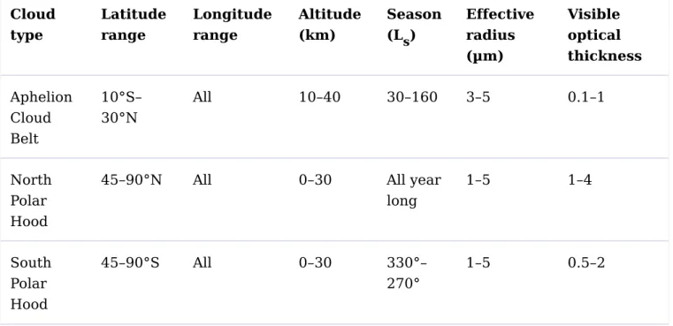
2003) from the Infrared Thermal Mapping (IRTM) data of the Viking orbiters. This study was, however, lacking the analytical means to extract quantitative cloud characteristics beyond the capability to detect cloud presence by their induced contrast of brightness between two separate radiometric channels. Nevertheless, this study opened the path to an era of a systematic survey of water ice clouds in the Martian atmosphere whose canonical view (see Table 1) is widely recognized as having been assembled out of the MGS Thermal Emission Spectrometer (TES) data (Pearl et al., 2001; Smith, 2004; Smith et al., 2001). TES achieves a spatial resolution of 3 km across track and 10–20 km along track, which prevents sampling the cloud structure at sub-kilometer scale, contrarily to visible images. TES cloud climatology (from 2001 to 2009) was derived from nadir measurements and has later been complemented by similar measurements from the Planetary Fourier transform Spectrometer (PFS) (Giuranna et al., 2019).
Table 1. Summary of the Main Martian H O Ice Cloud Manifestations and Their Observed Properties Cloud type Latitude range Longitude range Altitude (km) Season (L ) Effective radius (µm) Visible optical thickness Aphelion Cloud Belt 10°S– 30°N All 10–40 30–160 3–5 0.1–1 North Polar Hood
45–90°N All 0–30 All year
long 1–5 1–4 South Polar Hood 45–90°S All 0–30 330°– 270° 1–5 0.5–2 2 s
The TES Monitoring Era
Whereas water ice clouds were long identified essentially by their whitish optical properties in the visible, TES provided the first unambiguous means to distinguish them from the
surrounding dust, thanks to the 12 μm (825 cm ) infrared absorption/emission of water ice. In a way similar to the monitoring of dust opacity with the 9 μm band produced by silicate material, it has been possible since the early use of TES to build up a water ice cloud
climatology revealing the seasonal behavior of clouds over a large part of the Martian globe (Figure 1, left panel). Fitting the 12 μm band of water, Smith et al. (2001) were able to
estimate the vertically integrated opacity of the water ice clouds and to establish its intimate link to temperature in the Martian atmosphere. The inclusion of cloud opacity as part of the standard products of the TES instrument along with dust opacity, water vapor, and the atmospheric temperature has framed the classical organization of the main Martian climatic parameters, which water ice clouds were eventually found to be an integral part of.
Since TES, other instruments have contributed to the climatology of water ice clouds on Mars, such as ACS and NOMAD on the Trace Gas Orbiter (Fedorova et al., 2020; Liuzzi et al., 2020; Stcherbinine et al., 2020), THEMIS (Smith, 2019) on Mars Odyssey, MCS (McCleese et al.,
2010), MARCI (Clancy et al., 2016; Wolff et al., 2019) on MRO, SPICAM (Montmessin et al.,
2017; Willame et al., 2017), OMEGA (Madeleine et al., 2012; Olsen et al., 2019), and PFS (Giuranna et al., 2019) on the Mars Express mission, as well as in situ information delivered by the Phoenix (Whiteway et al., 2009) and the MSL (Kloos et al., 2016; McConnochie et al.,
2018) missions.
While clouds have been observed at almost all seasons and latitudes (see Figure 2), their occurrence has been observed to follow a seasonally recurrent pattern from which two
prominent classes emerge: the Aphelion Cloud Belt (ACB) and the Polar Hood (PH) clouds (see Figure 1). These events are the prevalent features of the cloud annual cycle (Liu et al., 2003), with very little interannual variability recorded for the ACB, the latter being by far the best documented of the two classes of clouds. Both are planetary-scale cloud formations that exhibit distinct properties discussed in the following sections.
Figure 2. (Left) A compilation of the zonally averaged water ice cloud opacity in the infrared
as inferred from the TES and THEMIS infrared spectrometer observations. The presence of the Polar Hood can be sensed at the border of the polar night in the fall–winter of both
hemispheres. Reprinted with permission from Clancy et al. (2017). (Right) Same as left, except PFS data are represented and rearranged to compare the PH occurrence between the two hemispheres in their respective fall–winter formation season.
PFS data reprinted from Giuranna et al. (2019).
The Aphelion Cloud Belt
The ACB (also referred to as the equatorial cloud belt) occurs every year during northern spring and summer (L ~30 to ~150°) and covers the equatorial regions between 10°S and 30°N (see Figure 2). This distinct and recurrent Martian cloud feature was first identified by Clancy et al. (1996) from the Hubble Space Telescope (HST) images and later supported by Wolff et al. (1999) using the same asset. This peculiar cloud manifestation appears tightly synchronized to the annual temperature minimum encountered in the equatorial region as Mars revolves along the portion of its orbital trajectory that is the most distant from the Sun, forcing an annual minimum in solar input.
TES revealed that the ACB begins at the vernal equinox (L = 0°), progressively increases in opacity and in spatial extension up until L = 80°, and reaching typical optical depths of 0.15– 0.2 (at 12 μm) within the 10°S to 30°N latitudinal domain. Around L = 140°, the ACB starts its annual decline, disappearing by the autumn equinox at L = 180° (Smith, 2004).
The ACB is known to exhibit large diurnal variation of opacity. At night, the cloud cover is present at all longitudes, exhibiting a quasihomogeneous opacity. During the day, opaque clouds cluster near the topographic edifices of the Tharsis and Elysium regions, being mostly undetectable elsewhere. Indeed, locally, the ACB shows distinct increases in opacity (Benson et al., 2003) in relation with the presence of the main topographic edifices of the equatorial region (i.e., the volcanoes of the Tharsis Montes as well as one forming at the northern edge of the ACB in the Elysium region). It is interesting to note that in the southern hemisphere, a feature seasonally correlated to the ACB concerns the concentration of clouds in the Hellas basin that is peripheral to the southern boundary of the ACB (see Figure 3 of Giuranna et al.,
2019). The ACB shows also some hemispherical asymmetry with a more opaque cloud banding in the northern tropics than in the southern portion of the ACB. This pronounced latitudinal gradient of opacity is explained by the convergence of wet air masses carrying humidity from the subliming north polar cap and pooling in the tropical region dominated by ascending motion.
The Polar Hoods
PH clouds have not been characterized as extensively as those in the ACB. PH cloud
occurrence appears controlled by the latitudinal excursion and seasonality of the polar nights. For this reason, they have remained mostly excluded from nadir observations that rely on scattered sunlight in the visible and in the near-infrared. The low temperature (~140K) prevailing in these regions and the small thermal contrast between the surface and the
atmosphere make observations in the thermal infrared equally challenging. PH clouds form in the high latitudes of the fall hemisphere and appear strongly coupled to the seasonal
evolution of the CO caps at the surface and to the polar vortex in both hemispheres. As for
s s s s s 2
the ACB, PH clouds tend to occur in the regions encountering a seasonal decrease in
temperature, explaining the seasonal timing paced by the onset, stabilization, and demise of the fall-winter polar environment.
Previously, nadir surveys of PH clouds had been restrained to the fringes of the polar nights where illumination and temperature conditions favor their observation (Smith, 2004; Wang & Ingersoll, 2002) until PFS unveiled their presence deep in the polar nights, revealing a
striking asymmetry between the northern and the southern PH (Giuranna et al., 2019, see Figure 2, right panel), with distinctly thicker (up to an opacity of 1 at 12 μm) and more widespread PH clouds in the north. In addition, the north PH is present almost all year long, whereas the south PH is observed 65% of the year (as deduced from the cloud seasonal distribution shown in figure 9 of Giuranna et al., 2019). It remains unclear what drives this asymmetry apart from the obvious contrast of topography between the two hemispheres and the fact that the north picks up larger amounts of volatiles overall. PH clouds tend to be thicker than ACB clouds by a factor of 3–5, clustering at the equatorward edge of the polar night in both hemispheres.
Water Ice Cloud Vertical Distribution
Water ice cloud distribution with altitude has been documented by many orbital remote sensing experiments, starting with the first global survey derived from the Mariner 9 and the Viking missions (Anderson & Leovy, 1978; Jaquin et al., 1986). These observations had no capability to discriminate between widespread dust from icy particles, yet such discrimination could be tentatively made by considering the behavior of light scattered by the atmosphere at various altitudes. The work of Jaquin et al. (1986) is suggestive of the presence of water ice clouds in the form of discrete layers either detached or attached to the main structure of the profile shaped by the dusty haze. These discrete layers show a strong enhancement in
brightness disrupting the otherwise continuous appearance of the haze and potentially revealing the presence of more abundant and brighter material, such as water ice in the visible domain. While this assumption proved largely true thereafter, with confirmation brought by a number of missions, it was also found that dust could produce similar
protuberances in the profiles, arguably caused by enhanced convective activity (topography, storms) propelling dust higher and faster than the main circulation alone can do (Heavens et al., 2014; Spiga et al., 2013).
Vertical profiles showing evidence for clouds were also obtained during the Phobos mission using the solar occultation technique (Chassefière et al., 1992, Korablev et al., 1993, Rodin et al., 1997). Solar occultation relies on the total extinction (absorption + scattering) caused by particles lofted along the line of sight. As such, it is nearly independent of the particle shape and provides robust access to the particle properties. Since the Phobos mission, the
characterization of cloud profiles has been documented from the UV to the thermal infrared (Benson et al., 2010, 2011; Fedorova et al., 2009, 2020; Guzewich & Smith, 2019; Liuzzi et al.,
2020; Määttänen et al., 2013; Maltagliati et al., 2013; McCleese et al., 2010; Montmessin, Quémerais, et al., 2006; Rannou et al., 2006; Smith et al., 2013; Stcherbinine et al., 2020). The typical appearance of clouds can be represented by a 5 to 20 km thick layer overlying the dust layer at an altitude varying from the near-surface up to the upper mesosphere (80 km). Near-surface water ice clouds were first reported by the LIDAR experiment on the Phoenix
mission that operated in the northern polar region of Mars (Whiteway et al., 2009). The clouds observed there were untypical in that their retrieved properties, their particle size in
particular, strongly contrasted with what was known about water ice clouds at that time. Phoenix reported the formation of a kilometer-thick cloud lofted at 4 km, from which
intermittent separations of particles occur from below the cloud which resembled terrestrial virgae.
Besides Phoenix, Pathfinder, Mars Exploration Rovers, and Mars Science Laboratory (MSL) missions were productive assets at the surface of Mars for the characterization of water ice clouds. A number of works derived from MSL data led to the characterization of clouds as seen from the surface (Lemmon et al., 2015; Moores et al., 2015), with a dominant cirrus morphology.
Polar hood cloud profiling performed by the Mars Climate Sounder (MCS) suggests cloud stretch from 10 to 40 km in the north and slightly lower in the south (see Figure 3). Note that the MCS observing mode prevents reliable measurements in the first 10 km above the surface due to excessive tangential opacity.
Figure 3. Log of the zonal average water ice density-scaled opacity (m kg ) dayside retrievals for MY 29 for the L bins labeled at the top of each panel. Contours shown are every 0.1 log units. Note the pressure scale is between 1000 and 0.1 Pa. On Mars, two decades of pressure roughly correspond to 40 km of altitude difference.
Reprinted with permission from McCleese et al. (2010).
H O Ice Cloud Properties
So far, the most commonly reported values for water ice clouds particle radii range from 1 to 5 μm (Chassefière et al, 1992; Clancy et al., 2003; Fedorova et al., 2020; Guzewich & Smith,
2019; Luizzi et al., 2020; Madeleine et al., 2012; Olsen et al., 2019; Stcherbinine et al., 2020). It is to be noted that the reported values are in good agreement with the seminal predictions of Michelangeli et al. (1993), who theoretically bracketed the excursion of water ice crystal particle radii based on the first application of a detailed microphysical model to Martian atmosphere conditions. This range of values can be qualitatively understood as the result of
10
2 −1
s
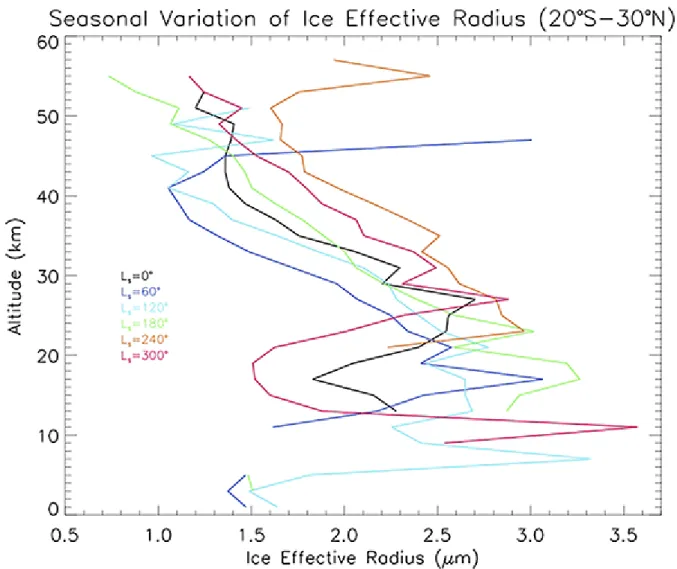
an average amount of condensed water (10s of ppmv) distributed over the average number density of dust particles (1–10 cm ) lofted in the atmosphere. The resulting crystal radius has a power of 1/3 dependence on these quantities, which buffers the impact of the changes in water/dust on the radius of the crystal. This dependence probably explains the observed relatively small variability of this cloud property on Mars, considering terrestrial standards. In the intertropical region, water ice particle radii > 3 μm can be observed all year long and it peaks in size around the ACB occurrence period (see Figure 4). ACB cloud particles are the best documented type of clouds when it comes to their particle sizes. The ice crystals of the ACB have microphysical properties that have been estimated by several authors from remote sensing techniques and who established a range of values between 2 and 5 μm, (Clancy et al.,
2017). The apparent analogy with a particular type of particle found in tropospheric terrestrial cirrus clouds is supported by the comparable scattering behaviors (Yang et al.,
2003). These particles consist of equidimensional faceted ice particles, also known as droxtals (Wolff et al., 2011).
Figure 4. Zonal average of CRISM derived water ice cloud effective radius in the 20°S–30°N
latitude region binned by 60° of solar longitude.
Reprinted with permission from Guzewich and Smith (2019).
Elsewhere, particle radii ranging between 1 and > 3 μm have been reported (Guzewich & Smith, 2019; Figure 4) based on CRISM limb observations, establishing a strong variability within a restricted range of these values for any given altitude. However, one particular occurrence of clouds exhibited considerably larger values. The Phoenix mission, which operated at 68°N, witnessed a rare type of cloud forming around 4 km of altitude and consisting of precipitating water-ice crystals of < 30 μm in radius, behaving in a way
analogous to terrestrial virgae (Whiteway et al., 2009). This type of cloud formation has never been observed anywhere else on Mars and may have been the result of untypical conditions at the end of the northern summer season where the wet summer atmosphere near the surface encounters rapid temperature decrease, fueling cloud formation. Mesoscale simulations have later proposed a different explanation for the virga-like appearance of the observed cloud profile features: the role of local convective cells created by the cloud and capable of carrying ice particles much faster than sedimentation alone toward the surface (Spiga et al., 2017) and thus not requiring ice crystals to be as large as estimated by Whiteway et al. (2009).
CO Clouds
Polar CO Clouds
The Mariner 7 flyby acquired precise information on the composition of the Martian polar caps, and both temperatures allowing for CO condensation and CO ice itself were detected (Herr & Pimentel, 1970; Neugebauer et al., 1969, 1971), proving that this volatile could condense as ice, at least at the surface in the polar night. Simple models of the thermal state of the polar night atmosphere had also shown that CO condensation should be possible and that the atmosphere should also be thermodynamically in equilibrium with the surface condensates, and thus in a saturated state. This was putatively observed in the Mariner 6 flyby exit radio occultation acquired at high northern latitudes that showed atmospheric temperatures close to saturation near the surface, and that the atmosphere was
supersaturated also above 10 km altitude (Hogan et al., 1972).
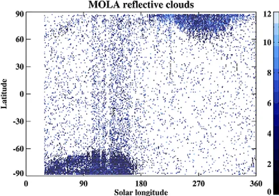
The detection of plausible CO clouds remained a challenge until very late. Only at the end of the 1990s were polar CO clouds indirectly detected by the Mars Orbiter Laser Altimeter (MOLA, on the Mars Global Surveyor satellite, MGS) (Ivanov & Muhleman, 2001; Pettengill & Ford, 2000) and mapped using the same instrument (Neumann et al., 2003). MOLA LIDAR was an active ranging instrument conceived to measure the Martian topography and, as a side product, to detect Martian clouds through their reflective or absorbing properties. MOLA detected strong signals, laser echoes, coming from high above the surface within the polar nights. It was deduced that the echoes were coming from the tops of thick clouds, probably composed of CO crystals. The probable CO composition of the clouds was deduced from the known fact that CO was condensing at the surface during the same season, and from very low measured atmospheric temperatures indicating that atmospheric condensation was plausible (Ivanov & Muhleman, 2001; Pettengill & Ford, 2000). The clouds mainly formed below 10 km, but some signals were received even from an altitude of 20 km. The polar cloud top structures revealed by adjacent echoes were reminiscent of sloping buoyancy wave fronts. MOLA observed these clouds during one Martian year (see Figure 5). The MOLA
measurement range was designed so that only returns within a certain range of the actual 2 2 2 2 2 2 2 2 2 2
expected surface were measured (maximum 40 km) and, because of this limitation,
mesospheric clouds could not be detected by MOLA. No composition information of the clouds could be retrieved either.
Figure 5. MOLA cloud returns observed above the Martian surface (color, in kilometers) as a
function of latitude and solar longitude, averaged in a grid of 1º × 1º.
Data from Neumann et al. (2003), downloaded from NASA’s Planetary Geology, Geophysics, and Geochemistry Laboratory <https://pgda.gsfc.nasa.gov/products/62>.
MOLA revealed the existence of the polar clouds, but it was particularly difficult to acquire more data on the polar clouds that hide in the shadows of the very cold polar night and have very low thermal contrasts with respect to the surface ice. A decade after the MOLA
observations, the MCS radiometer on the Mars Reconnaissance Orbiter (MRO) mission probed the Martian polar nights and was able to shed more light on questions related to CO
condensation and possible snowfall in the polar night. MCS is a thermal emission and visible radiometer that has good spatial coverage, functions in limb mode, thus disposing of the surface–atmosphere thermal contrast problem of nadir observations, and has a particular scanning strategy allowing the observation of the polar regions. MCS measured the radiative cooling rates in the polar night and, with hypotheses on particle sizes, deduced that 3–20% by mass of the seasonal polar cap CO might be deposited by snowfall (instead of direct
condensation onto the ground) coming from the lowest (below 4 km) atmosphere (Hayne et al., 2012, 2014).
Combining MOLA, MCS, and MGS Radio Science, Hu et al. (2012) conducted a
comprehensive, multi-instrument study on polar atmospheric CO condensation, providing causal evidence that the MOLA atmospheric returns were associated with CO condensation. They also mapped the seasonal variations of atmospheric saturation, finding hemispheric and
2
2
2
interannual variations. They estimated the condensed mass and precipitation flux at each pole constraining the cloud crystal radii. At the beginning of the 21st century, this observational study was the most comprehensive one on the polar CO clouds.
MOLA and MCS are complementary; using the spatial and temporal distributions combined, a fairly good three-dimensional (3D) view (on average, since they did not observe on the same Martian Years) of the polar clouds can be constructed. The observations by MOLA and MCS thus give the only observational constraints known for the moment on the polar CO clouds (Table 2): occurrences, cloud top heights and their structures, estimates on particle sizes and optical thicknesses, radiative cooling rates that can be converted into condensed mass, and estimates on the fraction of the seasonal CO cap deposited as snowfall. The polar CO clouds form on both poles during the local polar night, between the surface and 15–20 km altitude, host crystals with 1–100 µm effective radii, and have an optical thickness of 0.1–100. Several lines of evidence point to differences in cloud processes and properties between the poles.
Mesospheric CO Ice Clouds
The Martian mesosphere is the atmospheric region between approximately 40 and 120 km, and very cold temperatures, close to the CO condensation temperature, can be reached in mesospheric altitudes, particularly near the equator. Early on in the Martian exploration, the Mariner 6 and 7 spectrometer limb observations of the atmosphere at low latitudes revealed a spectral peak in the near-infrared, around 4.26 µm, characteristic of CO ice, and it was deduced that CO clouds had been observed in the Martian atmosphere (Herr & Pimentel,
1970). However, the observation came from the lower atmosphere, at around 25 km altitude, but seemed to indicate that atmospheric CO condensation was possible at low latitudes. Later on, this observation was attributed to an emission caused by the gaseous atmospheric CO (Lellouch et al., 2000) and not by CO ice clouds. Nevertheless, Mariner 6 and 7 radio occultation profiles all showed clear supersaturation with respect to CO in the middle
atmosphere (above 30 km at mid and low latitudes and above 10 km in high latitudes) (Hogan et al., 1972), and some of the coordinates of these observations corresponded quite closely to those of the spectrometer observations of the 4.3 µm emission (Herr & Pimentel, 1970). Also, the Mariner imaging experiment observed detached haze layers on the planet (Leovy et al.,
1971).
Around the time of the MOLA discovery of the polar CO clouds, Clancy and Sandor (1998) hypothesized, based on ground-based temperature measurements, the Mars Pathfinder descent profile (Schofield et al., 1997), and one image taken from the surface by the Mars Pathfinder showing bluish, predawn clouds high in the atmosphere, that CO ice cloud formation was also plausible in the mesosphere. Soon thereafter, Clancy et al. (2003, 2004) began reporting sightings of high-altitude detached layers in limb observations by the MOC and TES on MGS.
Some years later, detached haze layers adjacent to temperature excursions below the CO condensation point were observed in SPICAM/Mars Express (MEX) stellar occultation profiles (Montmessin, Bertaux, et al., 2006). Layers were detected in only four profiles, but the
evidence pointed to very thin, subvisible (visible optical thickness ~0.01) CO clouds composed of small crystals (~100 nm effective radius).
2 2 2 2 2 2 2 2 2 2 2 2 2 2 2 2
Two instruments, MOC and TES, on MGS continued to observe detached layers of aerosols at high altitudes (60–80 km) in limb observations on the dayside of the planet, and a climatology of these Mars equatorial mesospheric (MEM) clouds was compiled (Clancy et al., 2007). The instruments MOC and TES detected and mapped these layers forming near the equator during the northern hemisphere spring and summer. The layers were fairly certainly ice clouds with effective radii in the micrometer range, but it was not possible to distinguish between H O and CO ices with the available observations. Subsequently, Inada et al. (2007) reported on a handful of THEMIS/Mars Odyssey visible image observations of mesospheric clouds above 45 km around the equator and above 70 km at the terminator.
Simultaneously, the OMEGA instrument on MEX made the first confirmed spectroscopic detection of CO ice clouds in nadir observations (Montmessin, Gondet, et al., 2007) after hints from the PFS instrument on MEX (Formisano et al., 2006). The clouds were identified thanks to their spectral signature at 4.26 µm, which was shown by radiative transfer
calculations to appear in OMEGA nadir spectra only if the CO crystals that scattered the photons were residing above 40 km. These observations provided definitive proof on the formation of mesospheric CO clouds on Mars. The first 1-year climatology (Montmessin, Gondet, et al., 2007) was followed by a 3-year survey (Määttänen et al., 2010) combined with High-Resolution Stereo Camera (HRSC/MEX) images of mesospheric clouds (Scholten et al.,
2010), identified in some cases as CO clouds by simultaneous OMEGA observations.
McConnochie et al. (2010) looked more into the THEMIS-VIS observations reported by Inada et al. (2007) and reported on equatorial mesospheric clouds and a new midlatitude cloud class: The latter was also seen in OMEGA and HRSC observations (Määttänen et al., 2010; Scholten et al., 2010). These clouds were mainly observed at twilight at northern midlatitudes. McConnochie et al. (2010) performed radiative transfer retrievals on a subset of equatorial clouds and showed that CO composition was preferred over water ice.
THEMIS-VIS and HRSC (McConnochie et al., 2010; Scholten et al., 2010) are both able to determine the cloud altitudes thanks to parallax in subsequent images. In addition, due to a time delay between the images, the cloud displacement in the direction perpendicular to the orbit can be interpreted as an indicator of mesospheric winds. The altitude determinations, and most importantly, the related wind estimates provide unique data on the Martian
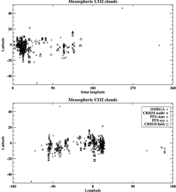
mesosphere that have been used later on to constrain models (Gonzalez-Galindo et al., 2011). Since these first climatologies, mesospheric clouds have been observed in many other data sets as well (see Figure 6). CRISM on MRO distinguished CO clouds in nadir images by ruling out H O composition in the absence of a water ice signature (Vincendon et al., 2011), MCS/ MRO mapped high-altitude layers in thermal infrared limb observations with no definitive composition analysis (Sefton-Nash et al., 2013), IUVS/MAVEN detected mesospheric aerosol layers in scattered sunlight at the limb (Stevens et al., 2017), and PFS/MEX published a 5-year nadir climatology of CO clouds (Aoki et al., 2018), identified thanks to the same CO ice spectral feature at 4.26 µm as with OMEGA. In addition, Clancy et al. (2019) analyzed CRISM/ MRO limb profiles to detect mesospheric clouds and their composition. They also compared their results to near-simultaneous MCS/MRO and MARCI/MRO observations, providing a context for the interpretation. Jiang et al. (2019) added to the cloud climatology two high-
2 2 2 2 2 2 2 2 2 2 2
altitude detached aerosol layers coinciding with a CO -supersaturated cold pocket. These two clouds were unique in their season of observation: They were observed with IUVS/MAVEN during summer at low southern latitudes.
Figure 6. Published mesospheric CO cloud data sets. These include only the observations
by instruments that have provided a confirmed detection of CO ice. Top panel: Solar
longitude-latitude map. Bottom panel: Longitude-latitude map. References related to the data sets are as follows: OMEGA: Määttänen et al. (2010) and Vincendon et al. (2011); CRISM nadir: Vincendon et al. (2011); PFS: Aoki et al. (2018); CRISM limb: Clancy et al. (2019).
According to the observations acquired during the two first decades of the 21st century, the mesospheric clouds form preferably around the equator in northern spring and summer, and on some rare occasions at (south and north) midlatitudes during the local autumn. The majority of the observed clouds are daytime clouds that form around 40–80 km altitude. The predominance of daytime cloud observations may be due to the observational methods dominated by visible or near-infrared observations of reflected sunlight. Nighttime clouds around 100 km were detected by the SPICAM UV spectrometer in stellar occultations, but only in a handful of profiles out of several hundreds. Such clouds were detected also in stellar occultations by the IUVS instrument on the MAVEN satellite. Despite the scarcity of the
2
2
nighttime observations, the upward propagation of the strong Martian thermal tide gives a logical explanation for the different cloud formation altitudes during day and night. Overall, the daytime clouds are found at lower altitudes, they are optically thicker (visible optical thickness maxima around 0.5), and the effective radii found are larger (0.5–3 µm), whereas the nighttime clouds are at higher altitudes, optically very thin (subvisible: 0.01), and their effective radii are around 100 nm. See Table 2 for a summary of observations.
Table 2. Summary of Martian CO Clouds and Their Observed Properties, Listed by Type
Cloud type Latitude
range Longitude range Altitude (km) Season (L ) Effective radius (µm) Visible optical thickness Polar tropospheric CO 65–90° All 0–20 Polar winter 1–10s 0.1–1 Midlatitude mesospheric (CO ?) 40–50°N 55–40°S N: 290– 340°E S: 90– 220°E 40–70 Local autumn 0.1–1.5 < 0.5 Equatorial mesospheric (CO ?) 40°S– 20°N -120°E– 30°E 90°E, 150°E 45–100 330– 85°, 100– 160° 1–3, 0.1 < 0.5, 0.01 2 s 2 2 2
State of the Art of the Martian Clouds
No Mars mission has been solely dedicated to clouds, but atmospheric phenomena have been an important objective, leading to advances in Martian cloud studies as well. Practically all missions perform retrievals of the atmospheric state for interpreting observations and for reaching some other goals (e.g., removal of atmospheric effects for surface studies), providing information on clouds in the atmosphere. Thus, an ample number of data sets on clouds has been acquired during the decades of Mars exploration. These retrievals often involve complex radiative transfer calculations requiring detailed data on the optical properties of the
substances, readily available for Martian ices whose refractive indices have been well documented. Observations, theoretical work, and laboratory experiments have helped in defining their microphysical characteristics, such as crystal habits, particle size ranges, ice densities, and the contact parameters of ices on different substrates, very important for modeling the formation of clouds. Modeling aspires to fill in the gaps left by observations and to interpret observed but unexplained phenomena, and models also need to be validated by comparing them with observations. These tasks require complex models, including detailed cloud microphysics providing the coupling of clouds with atmospheric temperatures, and preferably, in addition, with radiative effects and associated feedbacks. The inclusion of clouds in Martian climate models has taken great leaps from the early 2000s. In the following, the current state of understanding of Martian clouds is described.
Water Ice Clouds in the 21st Century
The growing interest of the community in the role of water ice clouds in the climatic system of Mars is echoed by the significant increase at the change of the century of publications in relation to clouds, both from an observational and a theoretical standpoint.
Kahn (1990) was the first to invoke water ice clouds as an active part of enhanced
sequestration of water in the regolith. Indeed, water condensation into ice crystals blocks water vapor from further upward propagation, and subsequent sedimentation and evaporation recycles these ice particles back into water vapor below the cloud formation level. In this way, clouds tend to confine water vapor closer to the surface and stimulate exchanges of water between the regolith and the atmospheric layers overhanging it. This near-surface
confinement was hypothesized to explain the premature moistening of the midlatitude regions at a season where the sublimation of the north polar cap, the main reservoir of water at the surface, had not begun. Later work proved this premature moistening was instead the result of the sublimation of seasonal frost accumulated along the edge of the polar nights during fall and winter (Houben et al., 1997; Richardson et al., 2002), a mechanism that also proved to be controlled by clouds (Montmessin et al., 2004).
Following their first observation of the Aphelion cloud belt, Clancy et al. (1996) proposed a mechanism that has been referred to as the Clancy effect. The Clancy effect consists of an asymmetric pump between hemispheres favoring the long-term accumulation of water in the north.
This effect was extrapolated from the expected impact of the ACB during spring and summer in the northern tropics at a time when the tropical circulation is dominated by the uprising motion of the solstitial Hadley cell. Inside the upward branch of the cell, air masses are adiabatically cooled, promoting condensation and explaining the observed widespread cloud formation. However, water appears sequestered in this pattern as cloud formation implies that a fraction of water is confined below the condensation level instead of rising further along the Hadley cell streamlines that should theoretically transfer water vapor to the south (Figure 7). The opposite situation in southern spring and summer contrasts with a much higher elevation of the condensation level, which basically lets water vapor free to incorporate the most
intense portion of the Hadley cell and be transferred seamlessly northward. As this
mechanism operates only around aphelion season (northern spring–summer transition) when Mars is most distant from the Sun and its equatorial atmosphere experiences its coldest state year round, the long-term net effect of the ACB in the water distribution at the surface of Mars is an accumulation of water in the north polar region where the most extensive
permanent reservoir of water ice can be spotted at the surface. This effect was validated 10 years later by 3D models (Montmessin et al., 2004; Richardson et al., 2002) and was also shown to reverse at times of opposite perihelion orbital configuration, which takes place every 150,000 years (Montmessin, Haberle, et al., 2007) when the south polar region is favored for long-term accumulation.
Figure 7. Meridional cross-section water advection patterns simulated for the aphelion
period (northern spring-summer, L = 90°). Color contours are coded according to water vapor concentrations (purple, 1 ppm, to orange, 250 ppm). Streamlines showing the
orientation of the atmospheric circulation are indicated by solid and dashed lines; values refer to the streamline intensity (10 kg s ). Red diamonds indicate the presence of water ice clouds.
Reprinted with permission from Montmessin, Haberle, et al. (2007).
The inclusion of clouds as an active radiative agent in 3D climate models has enabled the identification of a number of cloud-induced radiative phenomena. ACB clouds are now
recognized to cause tropical warming of the middle atmosphere (Madeleine et al., 2012) as a result of water ice cloud absorbing the surface thermal emission. This warming is predicted by models to cause in return an intensification of the northern spring–summer Hadley
circulation, although models may overly amplify this effect (Navarro et al., 2014). A series of contributions unfolded this pioneering study that has exposed the role of water ice clouds in a variety of Martian climate characteristics (Haberle et al., 2019; Kahre et al., 2015; Navarro et al., 2014; Neary et al., 2020; Shaposhnikov et al., 2019; Spiga et al., 2017), making them one of the most actively studied components of the Martian climate system.
Other cloud-induced radiative effects have been identified, such as the enhanced nighttime deep convection mechanism subsequent to the static instability triggered by cloud infrared cooling and observed at a variety of places on Mars (Spiga et al., 2017). PH clouds are suspected to amplify latitudinal and longitudinal contrast of temperature within the polar night, leading to increased activity of eddies, which intensifies midlatitude weather phenomena (Haberle et al., 2019).
Overall, water ice clouds can be seen as a booster of global Mars’ climate activity, which tends to excite dynamical and radiative phenomena in a climatic background otherwise controlled by CO atmosphere interactions with radiation and airborne dust. It appears that their
exponential relation to temperature, through the Clausius–Clapeyron law, leads them to inject high doses of nonlinearity in the Mars’ climatic system, with the side effect of creating
instability in 3D climate model predictions (Navarro et al., 2014).
It is widely acknowledged that Mars’ climate cannot be reproduced successfully without a detailed and faithful representation of the water ice clouds (Table 1). Models suggest that a cloud representation involving the known microphysical processes (nucleation, scavenging of dust, condensation, sedimentation) at work is a prerequisite to reproduce Mars’ climate. However, despite their considerable influence on climate, the cloud global effect is
outmatched by that of dust, which has a stronger, more permanent, and more widespread action on radiative transfer and energetic balance of the Martian atmosphere.
CO Clouds in the 21st Century
Nearly two decades of observations have gradually increased our knowledge and
understanding of Martian CO clouds (see Table 2). Modeling predicted the cloud formation that was later confirmed by observations, and it has consequently helped in interpreting the observations and refining estimations of certain variables.
s
6 −1
2
2
The dynamical nature of the polar CO clouds has remained a mystery but has been explored by modeling. Even in the early days of Mars exploration, theoretical modeling studies,
although not accounting for all climatic factors, showed that CO frost point temperatures might be reached in the Martian atmosphere (Paige & Ingersoll, 1985; Pollack et al., 1981,
1990). Later on, polar cap balance and simple atmospheric condensation were successfully incorporated into global climate models (Forget et al., 1998; Hourdin et al., 1993, 1995; Pollack et al., 1993), allowing for a simplified simulation of the polar CO clouds. Then, inspired by the findings of MOLA, the first detailed studies on CO cloud formation with microphysics in the polar night were performed by Tobie et al. (2003) and Colaprete et al. (2003). Tobie et al. (2003) used an inelastic two-dimensional model to show through simulations with idealized topography that gravity waves initiated by orographic troughs could form clouds that were tilted against the wind direction, as observed. The successive clouds were formed by similarly successive topographic troughs instead of a trapped lee wave. Their simulations using realistic topography revealed a dependence of the cloud formation on wind direction (up- or downslope) but showed good overall agreement with MOLA observations. Colaprete et al. (2003) attempted to explain, using a one-dimensional microphysical model with a convective scheme, the hemispheric differences in MOLA observations with clearly more reflective clouds in the south than in the north. They
concluded that the southern polar night was more prone to convective instabilities: The higher topography in the south, the cooler temperatures and faster cooling of the air, and possibly larger ice nucleus (dust) concentrations were the reasons for the creation of the highly reflective southern clouds observed by MOLA in contrast with the less reflective ones of the northern polar night. Later, Colaprete et al. (2008) performed global simulations, including microphysics (NASA Ames Mars GCM), concentrating on the polar clouds and their convective potential (Convective Available Potential Energy, CAPE). The model results were compared to cloud observations and calculations of CAPE based on retrieved temperature profiles from MGS–TES observations.
The discovery of the mesospheric CO clouds at the change of the century was not a surprise as such, since their existence had been suspected for quite some time. What was more
surprising was some of their properties, such as the high maximum opacities reached and the particle sizes in the micron range of the daytime clouds (Montmessin, Gondet, et al., 2007), indicating large fall speeds in the thin mesospheric air. There are observations of mesospheric clouds from several instruments, and many data sets exist from visible imaging in several bands (cameras and spectral imaging instruments), thermal emission measurements, near- infrared spectrometry, (ultraviolet) occultations, and thermal infrared radiometry. The observations have been acquired in nadir and limb observations (including occultations). However, these data sets are very heterogeneous in spatial and temporal coverage, in
resolution, and in retrievable parameters. In particular, interannual and diurnal variations are for the moment practically impossible to discern because of uneven coverage.
The detection of these unique mesospheric clouds (which form out of the main constituent of the atmosphere) inspired modelers as well. Colaprete et al. (2008) included detailed cloud microphysics in a global climate model of the current Martian atmosphere. Although the Colaprete et al. (2008) model (NASA Ames) performed well at the poles, and they did predict mesospheric clouds, the modeled mesospheric cloud distribution did not (in hindsight) fit the observed one very well. The 2010s finally confirmed, in several separate studies, the
hypothesis originally proposed by Clancy and Sandor (1998) that the mesospheric clouds
2
2
2 2
formed in cold pockets created by the superposition of planetary-scale thermal tides and mesoscale gravity waves. Gonzalez-Galindo et al. (2011) showed with the LMD Mars Global Climate Model (MGCM) that the mesospheric temperature structure, dictated in particular by migrating and nonmigrating tides, explained very well the spatial and seasonal distribution of the clouds. Spiga et al. (2012) showed that the zones where gravity waves (GWs) could reach the mesosphere correlated very well with the zones where mesospheric clouds had been observed. These two studies, put together, explained why the mesospheric clouds mostly form in the tropics and showed that GWs must play a role in their formation. Yigit et al. (2015) showed, with a GCM incorporating a GW parameterization, that GWs have a strong effect on the temperature fields in the upper mesosphere as well, around and above 100 km, and particularly during the night and near the poles where very few or no clouds have been observed.
Listowski et al. (2013, 2014) developed a detailed microphysical model in one dimension (vertical atmospheric column) and were successful in reproducing daytime mesospheric CO clouds with effective radii and opacities as observed. However, reaching the observed opacities required adding a condensation nucleus source in the mesosphere. The sensitivity tests of Listowski et al. (2014) showed that dust, lifted from the planet’s surface and
omnipresent in the lower atmosphere, is not present in sufficient quantities in the mesosphere to be able to function as the sole source of condensation nuclei for mesospheric clouds. An exogenous source, mimicking the formation of meteoric smoke particles (MSPs), seemed a realistic possibility, which was later also suggested in relation to the lower altitude water ice clouds (Hartwick et al., 2019). However, MSP analogue particles have quite low contact parameters for CO (Nachbar et al., 2016), pointing to a higher nucleation barrier than expected and requiring very high supersaturations for nucleation to occur. The nucleation potential of the meteoric particles was further investigated in a study by Plane et al. (2018), who showed, based on MAVEN observations and modeling, that meteoritic magnesium atoms deposited in the mesosphere were transformed on Mars into hydrated magnesium carbonate agglomerates (or “dirty ice”). These nanometer-sized icy particles can function as very
efficient IN for the mesospheric clouds, since their contact parameter would be equal, or very close to that of CO ice on H O ice, which has been measured (Glandorf et al., 2002) and is more favorable for nucleation than that for MSPs (Nachbar et al., 2016).
The versatility of the observations gives a solid basis for studying the mesospheric clouds, but the heterogeneity of the data sets has proven to be a caveat when investigating interannual variations, a crucial element of a climatological time series. This is a consequence of most of the Mars missions having the atmosphere only as a secondary objective. As the Mars Climate Sounder (MCS) was designed as a purely climatological instrument, it may be able to shed light on this matter if its observations of high-altitude aerosol layers (Puspitarini et al., 2016; Sefton-Nash et al., 2013) can be analyzed to also retrieve composition information.
Open Questions
Despite the tremendous progress made in the 2000s and 2010s in our understanding of why and where water ice clouds form on Mars, a number of outstanding questions remain. For instance, nucleation, the starting point of water ice cloud formation, relies on the so far unverified assumption that dust particles have a good wettability, which facilitates the
2
2
formation of ice germs. This pragmatic assumption was inspired by considering the available “ingredients” (dust particles, water vapor) that Mars disposes of. Still, the affinity between dust and ice germs, symbolized by the so-called contact parameter, first used in Mars cloud studies by Michelangeli et al. (1993), has been a recurrent topic of dedicated laboratory and statistical analysis (Iraci et al., 2010; Määttänen & Douspis, 2014; Santiago-Materese et al.,
2018; Trainer et al., 2009) without delivering a firm consensus on its actual value and dependence. There might be a variety of substrates apart from dust that are involved in the nucleation of water ice (such as chlorine salts; see Santiago-Materese et al., 2018), but climate models have conservatively obeyed the canonical assumption that only dust particles serve as nucleation seeds.
Another source of uncertainty is the temporal and spatial scales water ice clouds are associated with. Both become major challenges when water ice clouds are introduced into Mars climate models that impose tight constraints on time-stepping and spatial gridding to represent the temporal and 3D structure of clouds. Cloud processes span a wide range of timescales, from a fraction of a second for nucleation to months for particle accretion mechanisms (Michelangeli et al., 1993). In 3D models, this variety of timescales requires management of the cloud physics separately from the rest of the other physical processes (radiative transfer, convection) to guarantee a faithful prediction of cloud characteristic evolution and of their radiative feedback. The problem of spatial scale has been explored in the horizontal dimension (Pottier et al., 2017) and did not prove to be of major importance. Yet, clouds possess sharp interfaces along the vertical, and cloud formation might prove more sensitive to this dimension and the way it is represented in models. On Earth, the spatial scale of clouds is a classical problem that has been overcome by empirical approaches (subgrid parameterization) whose development has been guided by a dense observational network. Such a network being impossible to deploy on Mars might leave this question unconstrained for quite some time on the Red Planet.
Finally, while clouds may not be the prime climatic actor of present-day Mars, in the recent past this may not have been the case at a time when the orbital configuration of Mars was much different from today. The orbit of Mars is subject to the strong influence of Jupiter, making it chaotic and subsequently impossible to prognosticate up to more than 20 million years ago. Yet such a period of time encompasses the main periodicities of its orbital parameters, implying, for instance, that obliquity that controls insolation conditions at the poles evolved in a range from 15 to > 45°. Such variation and its effect on the water cycle has been theoretically explored (Forget et al., 2006; Levrard et al., 2004, 2007; Madeleine et al.,
2014) and revealed dramatic changes in the water-holding capacity of the Martian
atmosphere, generating water vapor concentrations 10 to 30 times greater than today, leading in turn to enhanced cloud formation. However, no model so far has successfully represented the climatic effect of water ice clouds in such a superhumid configuration. The capacity of clouds in present-day Mars to introduce a nonlinear feedback loop in the climatic system can be anticipated to become even stronger at high obliquity, generating an instability that the current sophistication level of Mars climate models is unable to handle. This likely explains why no study to date has ever been published on the high obliquity climate of Mars with interactive clouds. However, one can legitimately anticipate that the high obliquity climates encountered in the recent past may have been dominated by a water ice cloud influence.
Some of the open questions on the polar CO clouds are related to their role in the formation of the seasonal polar ice caps and in the structure of the polar vortex, to their “moist”
convective nature, and to the coupling of water and CO cycles via heterogeneous nucleation of CO onto water ice crystals. The two latter topics are also relevant for mesospheric clouds. The formation of the polar ice caps pilots the surface pressure cycle of the planet, since 25– 30% of the atmosphere condenses on each pole during the polar night. It is suspected that snowfall from the polar CO clouds might contribute by 5–20% to the formation of the polar caps (Hayne et al., 2014), and thus their role in the global CO cycle is not negligible. The latent heat released in condensation can locally fuel convective processes (“moist” convection; Colaprete et al., 2008) and, on a larger scale, influence the structure of the polar vortex and related atmospheric circulation (Kuroda et al., 2013, Toigo et al., 2017). Since the polar night also hosts water ice clouds that form earlier in the season at higher temperatures, water ice crystals can provide nucleation sites to the CO crystals forming at lower temperatures. This coupling of the two cycles might turn out difficult to quantify through observational means. One important debate related to the mesospheric CO clouds was on whether they were of a convective nature. Montmessin, Gondet, et al. (2007) had suggested that some clouds
appeared to have an appearance and forms (roundish or relatively equal horizontal spread in each direction and similar to the vertical reach) pointing to a convective origin, and the observed particle sizes were very large, pointing to strong vertical motions required for keeping them aloft. Määttänen et al. (2010) found more potential convective cloud candidates and performed calculations of the possibly attainable vertical velocities in the clouds,
assuming that all of the latent heat released in condensation of the total mass of the cloud, estimated from observations of cloud optical thickness, was converted into kinetic energy (via the relation of Convective Available Potential Energy and vertical velocity). It was shown that for the mesospheric clouds to be convective (i.e., for sedimenting ice crystals to remain aloft thanks to convective vertical movements), the convective cells would need to concentrate all the energy released by latent heat in condensation in a small volume of some tens to hundreds of meters wide. This meant that the clouds would be formed by several, small convective “fountains” within the cloud. Vincendon et al. (2011) showed, based on a simultaneous image pair from OMEGA and HRSC, that the coarse OMEGA resolution may smooth the cloud features in such a way that they might be interpreted as convective due to the aspect ratio of the features, whereas the higher-resolution HRSC image clearly showed a cloud formed of stripes or filaments. The question is still open and will require high-resolution modeling of mesospheric clouds to be definitively answered.
Another question on the formation of mesospheric clouds is the source of the ice nuclei, the particles onto which the ice crystals form. Modeling (Listowski et al., 2014) has shown that dust particles lifted from the surface of the planet by winds and lofted into the mesosphere by a dust storm will sediment out of the mesosphere very rapidly, and the very small amounts of the smallest remaining dust particles are not enough as ice nuclei to form clouds with
observed opacities, pointing toward the need for another ice nucleus source. Thus, the current evidence points to an exogenous source of ice nuclei (Listowski et al., 2014), either provided by meteoric smoke particles or by magnesium atoms formed after meteor ablation, which consequently form magnesium carbonates that are further hydrated and coagulate to form dirty ice particles (Plane et al., 2018). Such particles could also have properties favoring nucleation (Plane et al., 2018).
2 2 2 2 2 2 2
Conclusion
Clouds are tracers of atmospheric temperatures and thus also of atmospheric dynamics and radiative effects, since their formation and evolution are strongly dependent on the local temperature, with feedbacks to the climate. Cloud studies are thus crucial to the
understanding of the climatic system of a planet. This is testified, for example, by the evidence that water ice clouds on Mars have a strong influence on the thermal structure of the
atmosphere and thus the climate. In a more general sense, the recent climate simulations for Earth have revealed that clouds seem to be the key factor in amplifying the response of the climate system to an increase in CO concentrations (Zelinka et al., 2020). Studying these complex objects and their nonlinear interactions with the atmospheric state on other planets may help to refine our theories and models applied to our own planet as well.
Acknowledgments
The authors gratefully acknowledge R. T. Clancy, E. Sefton-Nash, and M. H. Stevens for sharing their cloud detections with them. They thank the two anonymous reviewers and the editor, Stephen Lewis, for constructive comments that helped in improving this article. The authors acknowledge support from the French space agency, CNES, and the national research center, CNRS.
Further Reading
Deeg, H. J., & Belmonte, J. A. (Eds.). (2018). Handbook of exoplanets. Springer Nature. Haberle, R. M., Todd Clancy, R., Forget, F., Smith, M. D., & Zurek, R. W. (Eds.). (2017). The atmosphere and climate of Mars. Cambridge University Press.
Mackwell, S. J., Simon-Miller, A. A., Harder, J. W., & Bullock, M. A. (Eds.). (2013). Comparative climatology of the terrestrial planets (pp. 393–413). University of Arizona Press.
Rossow, W. B. (1978). Cloud microphysics: Analysis of the clouds of Earth, Venus, Mars and Jupiter <https://doi.org/10.1016/0019-1035(78)90072-6>. Icarus, 36(1), 1–50.
References
Anderson, E., & Leovy, C. (1978). Mariner 9 television limb observations of dust and ice hazes on Mars <https://doi.org/10.1175/1520-0469(1978)035%3C0723:MTLOOD%3E2.0.CO;2>. Journal of Atmospheric Sciences, 35, 723–734.
Aoki, S., Sato, Y., Giuranna, M., Wolkenberg, P., Sato, T. M., Nakagawa, H., & Kasaba, Y. (2018).
Mesospheric CO ice clouds on Mars observed by Planetary Fourier Spectrometer onboard Mars Express <https://doi.org/10.1016/j.icarus.2017.10.047>
2
. Icarus, 302, 175–190.
Benson, J. L., Bonev, B. P., James, P. B., Shan, K. J., Cantor, B. A., & Caplinger, M. A. (2003). The seasonal behavior of water ice clouds in the Tharsis and Valles Marineris regions of Mars: Mars Orbiter Camera Observations <https://doi.org/10.1016/S0019-1035(03)00175-1>. Icarus, 165, 34–52.
2
Benson, J. L., Kass, D. M., & Kleinböhl, A. (2011). Mars’ north polar hood as observed by the Mars Climate Sounder <https://doi.org/10.1029/2010JE003693>. Journal of Geophysical Research, 116, E03008.
Benson, J. L., Kass, D. M., Kleinböhl, A., McCleese, D. J., Schofield, J. T., & Taylor, F. W. (2010).
Mars’ south polar hood as observed by the Mars Climate Sounder <https://doi.org/ 10.1029/2009JE003554>. Journal of Geophysical Research, 115, E12015.
Chassefiere, E., Blamont, J. E., Krasnopolsky, V. A., Korablev, O. I., Atreya, S. K., & West, R. A. (1992). Vertical structure and size distributions of Martian aerosols from solar occultation measurements <https://doi.org/10.1016/0019-1035(92)90056-D>. Icarus, 97, 46–69.
Clancy, R. T., Grossman, A. W., Wolff, M. J., James, P. B., Rudy, D. J., Billawala, Y. N., Sandor, B. J., Lee, S. W., & Muhleman, D. O. (1996). Water vapor saturation at low latitudes around aphelion: A key to Mars climate? <https://doi.org/10.1006/icar.1996.0108> Icarus, 122, 36–62.
Clancy, R. T., Montmessin, F., Benson, J., Daerden, F., Colaprete, A., & Wolff, M. J. (2017). Mars clouds. In R. M. Haberle, R. T. Clancy, F. Forget, M. D. Smith, & R. W. Zurek (Eds.), The
atmosphere and climate of Mars <https://doi.org/10.1017/9781139060172.005> (pp. 76–105). Cambridge University Press.
Clancy, R. T., & Sandor, B. J. (1998). CO ice clouds in the upper atmosphere of Mars <https:// doi.org/10.1029/98GL00114>
2
. Geophysical Research Letters, 25(4), 489–492.
Clancy, R. T., Sandor, B. J., Wolff, M. J., Christensen, P. R., Smith, M. D., Pearl, J. C., Conrath, B. J., & Wilson, R. J. (2000). An intercomparison of ground‐based millimeter, MGS TES, and Viking atmospheric temperature measurements: Seasonal and interannual variability of temperatures and dust loading in the global Mars atmosphere <https://doi.org/10.1029/1999JE001089>, Journal of Geophysical Research, 105(E4), 9553–9571.
Clancy, R. T., Wolff, M. J., & Christensen, P. R. (2003). Mars aerosol studies with the MGS TES emission phase function observations: Optical depths, particles sizes, and ice cloud types versus latitude and solar longitude <http://dx.doi.org/10.1029/2003JE002058>. Journal of Geophysical Research, 108, 5098.
Clancy, R. T., Wolff, M. J., Lefèvre, F., Cantor, B. A., Malin, M. C., & Smith, M. D. (2016). Daily global mapping of Mars ozone column abundances with MARCI UV band imaging <https:// doi.org/10.1016/j.icarus.2015.11.016>. Icarus, 266, 112–133.
Clancy, R. T., Wolff, M. J., Smith, M. D., Kleinböhl, A., Cantor, B. A., Murchie, S. L., Toigo, A. D., Seelos, K., Lefèvre, F., Montmessin, F., Daerden, F., & Sandor, B. J. (2019). The distribution, composition, and particle properties of Mars mesospheric aerosols: An analysis of CRISM visible/near-IR limb spectra with context from near-coincident MCS and MARCI
observations <https://doi.org/10.1016/j.icarus.2019.03.025>. Icarus, 328, 246–273.
Clancy R. T., Wolff, M., Whitney, B., & Cantor, B. (2004). The distribution of high altitude (70 km) ice clouds in the Mars atmosphere from MGS TES and MOC limb observations. Bulletin of the American Astronomical Society, 36, 1128.
Clancy, R. T., Wolff, M. J., Whitney, B. A., Cantor, B. A., & Smith, M. D. (2007). Mars equatorial mesospheric clouds: Global occurrence and physical properties from Mars Global Surveyor