A COMPUTER-BASED MODEL FOR INSPECTION PLANNING
by
ROBERT RONALD TRIPPI B.A., Queens College of the City University of New York
(1966)
SUBMITTED IN PARTIAL FULFILLMENT OF THE REQUIREMENTS FOR THE
DEGREE OF MASTER OF SCIENCE at the MASSACHUSETTS INSTITUTE OF TECHNOLOGY June, 1968 Signature of Author ... ,... Alfred P. Sloan School of Managem nt, May 17, 1968
Certified by ...
Thesis Supervisor
Accepted by ... ... ... ....
Chairman, Departmental Committee on Graduate Students
Archives
os.INST. TEC
JUL 29 1968
MITLibraries
Document Services
Room 14-0551 77 Massachusetts Avenue Cambridge, MA 02139 Ph: 617.253.2800 Email: [email protected] http://libraries.mit.edu/docsDISCLAIMER OF QUALITY
Due to the condition of the original material, there are unavoidable
flaws in this reproduction. We have made every effort possible to
provide you with the best copy available. If you are dissatisfied with
this product and find it unusable, please contact Document Services as
soon as possible.
Thank you.
Some pages in the original document contain text that
runs off the edge of the page.
A COMPUTER-BASED MODEL FOR INSPECTION PLANNING
by
Robert Ronald Trippi
Submitted to the Alfred P. Sloan School of Management on May 17, 1968 in partial fulfillment of the requirements for the degree of Master of
Science in Management
ABSTRACT
This thesis considers the problem of optimizing screening inspection ef-fort in a general multistage sequential production process. Some of the factors relevant to obtaining optimal inspection policies are first described. A mathe-matical model is presented which possesses sufficient generality to produce
in-teresting results, yet admits to a relatively simple solution. Thus, the pot-ential for handling moderately large problems is present in this model. The mathematical model has been programmed on M.I.T.'s time-sharing system for the
rapid solution and analysis of specific problems, and typical computational re-sults are discussed. Through the analysis of the structure of the model and the resulting optimal soltuions, several significant insights into the deter-minants of the.optimal placement of inspection points in the process are obtained,
including the relative insensitivity of total quality cost to a suboptimal placement of inspection points and the expected behavior of the optimal policy as a result of changes in process parameters. The difficulties involved in
treating more complex cases are also discussed, as well as possible extensions of the present model.
Thesis Advisor: Leon S. White
Assistant Professor of Management
Professor E. Neal Hartley Secretary of the Faculty
Massachusetts Institute of Technology Cambridge, Massachusetts 02139
Dear Professor Hartley:
In accordance with the requirements for graduation, I herewith submit a thesis entitled "A Computer-Based Model for Inspection Planning." I would like to take this opportunity to express my gratitude to Professor L.S. White for helping to provide me direction and motivation in the preparation of this thesis.
Sincerely,
Robert Ronald Trippi
-
-4-TABLE OF CONTENTS
Page
Chapter I - Introduction To The Problem . . .. .. . . . . . . . . . . . 7
Organization . . . . . . . . . . . .. . . . . . . . . . . . . . . . 7
Some General Remarks Concerning Quality Assurance . . . . . . . . . 7
Choice Of An Inspection Policy . . . . . . . . . . . . . . . . . . . 9
Chapter II - The Mathematical Model . . . . . . . . . . . .. . . . . . . 14
A Brief Review Of Relevant Literature . . . . . . . . . . . . . . . 14
A Variation Of White's Shortest-Route Model . . . . . - -. . . . . 15
The Physical Problem . . . . . . . . -. . - - - 16
Network Formulations . . . . - -. . . . - - - 18
Model I . . . . . . . . . . . . . . . .. . .. . . . . .. . . . . 19
Model II . . . . .. . . .. . . - - - -. . -. . . -. - - - - -. 21
Cost Structure . .. . . - -. . -. - - -. - - - -. .. 21
Network Solution . . . .. - -. . .. . -. - - - -. 29
Flexibility Of The Model . . . . . - -. .. . . . - - -. -. . . . 31
Chapter III - Programmed Implementation . . . . - - -. .. . - - - - -. 34
Computational Requirements . . . . -. -. -. - - -. - - - -. 34
Programs, Data Files . . . .. -. . . . - - - 35
Execution Sequence . . . . - - -. . .. . . - -. - - - -. 39
Choice of Solution Structure . . . . . . . . . . . . . .. . .. . . 41
Computational Experience . . . . . . . . . . . . .. . . . . .. . . 41
Computational Limitations . . . . . . . . . . . . . . .. . .. . . 44
Chapter IV - Experimental Results and Analysis . . . . . . . . . . . . . 46
Data Set I - Example - . . . .. . . .. . - - -. -. - - - -. . . 46
-5-Table of Contents Page
(Continued)
Data Set II - Sensitivity of Solution to Processing Costs . . . . . 56
Data Set III - Analysis of Fixed Inspection Costs . . . . . . . . . 57
Chapter V - Conclusion And Recommendations For Future Study . . . . . . . 61
Reflections on the Model . . . . . . . . . . . . . . . . . . . . . . 61
Promising Areas For Further Investigation . . . . . . . . . . . . . 63
References . . . . 67
- 6 -DIAGRAMS Diagrams Figure 1 Figure 2 Figure 3a Figure 3b Figure 4 Figure 5 Figure 6 Figure 7 Figure 8
Sequential Production Process . . . . Model I General Network Form . . - -Model II General Network Form . . . .
Network For 2-Inspector, 3-Stage Line File Structure. .. . . . . -. -. . Execution Sequence . . . . . . . . .
Computation Time . . . . . . . . . .
Data Set I Total Cost Curve . . . .. TQC Vs. Fixed Inspection Cost . . -
-Page 17 20 22 23 38 40 43 48 59 LISTS List of Variables . . . . . . . . . . . . . . . . . . . . . . . . . . . Computational Results, Data Sets I and II . . . . . . . . . . . . . . . Computational Results, Data Set III . . . . . . . . . . . . . . . . . .
33 47 58
CHAPTER I
INTRODUCTION TO THE PROBLEM
Organization
This thesis is organized into five chapters and one appendix. This in-troductory chapter is an attempt to put the manufacturing inspection problem in proper perspective to the totality of problems in the shop and to suggest some of the considerations that one ought to be aware of in designing an in-spection policy. In addition, a brief survey of relevant literature is pre-sented.
Chapter Two is a description of the mathematical model which is the basis of the experimental work done by the author. Chapter Three explains the structure of the computational system and discusses computational limita-tions. Chapter Four describes the results of several problem runs with dif-ferent data sets. Chapter Five is a commentary on the limitations of the model employed and suggests possibly significant related areas for future investigations.
The Appendix contains program listings and a brief description of each of the programs.
Some General Remarks Concerning Quality Assurance
Associated with virtually every production process are considerations concerning the quality of the product(s) outputted from the system. Even in those processes in which no apparent effort is expended in assuring a quality product, non-systematic, casual (perhaps visual) inspection is often an implicit, unavoidable part of the process. The present discussion will be limited to
--
8-those manufacturing processes in which a systematic inspection procedure or policy can be devised in order to attain some goal (produce the product at minimum total cost, produce zero defects, etc.). It is interesting to note
that under many problem formulations the quality aspects of the manufactur-ing system are embodied in both a goal statement (i.e. minimize total costs including the cost of assuring acceptable quality) and solution constraints (i.e. no more than X% defective finished products will be acceptable) simul-taneously.
At the outset, we will assume inspection (of raw materials, partially finished goods, component sub-assemblies, and finished goods) is the primary instrument available for assuring acceptable quality in the finished product. Therefore, it is assumed that the technical production process to be employed
is determined beforehand from considerations which are unaffected by a choice of inspection policy. Clearly, in the more general case, alternate manufacturing methods would affect both the frequency of defective operations occurring and the physical methods to be used in inspection.
The inspection policy chosen, as an integral part of the production pro-cess, will greatly affect other aspects of the system, such as facility
scheduling, workforce requirements, etc. In particular, inspections which take place between manufacturing stages occupy finite time intervals and may
thus be considered as operations in total facility scheduling. In this case the inspection policy must be determined before scheduling can take place.
Although optimal inspection policies may exist for flow- or job-shop situations in which items are manufactured in small or unit lots, it appears that the systematic determination of optimal inspection policies will be potentially most useful in those situations in which large lots of a product
- 9
-are produced at a time, due to the considerable collection of non-standard data and computational effort required, as will be seen shortly. The re-mainder of this thesis will be concerned with questions of "pure" inspec-tion, ignoring possible interrelationships of inspection policy with other facets of production management, and taking the technological manufacturing process as given and not subject to change while the inspection policy is
in effect.
Choice of an Inspection Policy
For the purposes of this paper the following definition of an inspec-tion policy will suffice:
An inspection policy is a statement of the defect types to be inspected for, the point within the production process at which inspection for each defect type is to take place, and the sampling processes to be employed.
We are not concerned here with the actual inspection or testing method used, whether it be mechanical, electrical, or visual. It is assumed that appropriate procedures can be devised by the engineering staff of the firm and that there are no choices to be made among alternate inspection proced-ures. What we seek is the allocation of inspection resources to each possible defect type at various points in the manufacturing process which will attain some predetermined goal. Sometimes an extreme solution, such as inspection of every operation immediately after execution or no inspection at all, will be optimal.
The factors affecting the choice of an inspection policy are of two general kinds: those associated with the manufacturing process (exclusive of inspection), and those associated primarily with inspection. Some factors associated with the manufacturing process which will in part
-10
-determine the selection of an inspection policy are the following: 1) The arrangement of stages. In the simplest case manufacturing
stages constitute a strictly-ordered sequence such that for any stage y there exists at most one stage such that x directly precedes y and there exists at most one stage z such that y directly precedes z. In more complex manufacturing situations assembly and partition operations may occur.
2) The defect-generating process. Defective operations may occur at manufacturing stages, thus imparting physical defects to the product. A defect generated at any one stage may be repairable at different costs, depending on its severity, or be non-repair-able. Additionally, defects generated at a stage may be either dependent or independent of defects occurring at other (preceding) stages. In order to define the problem fully, statements must be made about the defect-generating process at each stage. These statements are usually of a statistical nature, specifying a probability distribution for each stage, or multivariate dis-tributions for the case in which the defect-generating processes of several stages are dependent. For example, it may be observed that the defect-generating process at a particular stage can be modeled as Bernoulli with fixed parameter p, the probability of generating defect which is invariably non-repairable. The quantity 1-p would then be the probability of the operation being successfully executed.
The concept of a defect-generating process at each manufacturing stage can be broadened to include operations in which components
-11
-are added to an assembly. It may be known, through incoming sampling procedures or otherwise, that a component (ex. a re-sistor) taken at random has a certain probability of being defective (out of spec). Thus, adding a defective component to an assembly can be considered to be a defect generated at the stage. A stage consisting of an assembly operation might then generate a component-type defect, an operation defect, or both.
3) Physical limitations on inspection imposed by the manufacturing process. In some instances, inspection for a defect generated at a manufacturing stage is impractical or impossible. For ex-ample, it may be a simple matter to test for a defect type within an assembly up until its outer casing is added, but
impossible afterwards.
4) Processing costs. If a defect is discovered within an item which renders it unusable, any operations performed on the pro-duct after the defect occurred may be considered to be wasted and taken into account in determining an inspection policy.
5) Repair costs. Repairable defects may be repaired, usually at some cost.
6) Costs associated with the removal of worthless items or revenues gained from selling items no longer usable in the manufacturing process.
- 12_
Some aspects of the inspection process relevant to the choice of inspection policy are:
1) The accuracy of inspection. The inspector may not be perfect. Defects of type i when inspected for may be overlooked with probability a . Also, there may be unavoidable ambiguities associated with inspection. For example, an electrical test of a partially completed assembly may indicate that one of several sub-assemblies is not functioning properly, but addi-tional effort may be required to locate the defective component or wiring error within the correct sub-assembly.
2) Costs associated with inspection. Inspection costs may include labor, equipment, and utility costs. Some components of inspec-tion cost may be fixed, others variable.
3) The availability of inspection resources. These are resources in limited supply, such as qualified manpower, special testing equipment, etc.
The above variables associated with the total production process which must be considered in selecting an inspection policy are meant only to be suggestive. Many other factors could no doubt be added to the list.
In addition to the factors just discussed, the effects of outputting defective goods must be considered in the selection of an optimal inspection policy. Defective finished goods may be returned to the factory for repair or exchange, usually at some cost to the firm. Customers may be lost
temporarily or permanently, thus reducing future sales levels and profits. Certain legal restrictions on the quality of merchandise produced may apply.
~13
-In many instances it is company policy to maintain certain standards of quality although defects are unlikely to be observed by the consumer due to the nature of the product.
CHAPTER II
THE MATHEMATICAL MODEL
A Brief Review of Relevant Literature
The foundation of the most recent model-oriented papers is a result derived by Lindsay and Bishop (1964)l and White (1966)2 regarding the in-tensity of inspection effort to be applied at those points in a single-line production process where inspection is to take place for the cases of
non-repairable only and non-repairable only defect types, respectively. It has been shown that, under a fairly general cost structure including linear
costs associated with outgoing defective material and per-unit inspection costs, a function including the total of inspection-related costs will be minimized by an extreme point solution at each stage, i.e. by zero or 100%
inspection at each potential inspection point. This result will doubtlessly bring relief to many production managers, for 100% inspection at intermediate
production stages appears to be common in industry. For models employing fixed costs associated with supporting an inspection station, one might ex-pect this result to be further reinforced.
Pruzan and Jackson (1967)3 have employed the "no partial sampling" theorem in the development of a model of inspection in a simple sequence of production stages, from which a least-expected-cost solution can be ob-tained through use of dynamic programming. Immediately following each manufacturing stage is a potential inspection point. From the set of
potential inspection points a sub-set is chosen at which 100% inspection will take place. Each inspector then inspects for the defect types which may have occurred since the previous inspection point.
-15 ~
4
White (1967) has developed a more general model similar to that of Pruzan and Jackson. Here, however, the defect-generating stages are parti-tioned into two disjoint sets: those which generate repairable defects and those which generate non-repairable defects. The optimization problem is cast into a shortest-route form, which admits to a relatively simple solu-tion, and a formulation is given for constrained inspection resources.
It appears that future investigations of the inspection effort alloca-tion problem are most needed in the areas of:
1) more complex manufacturing processes including the admissibility of assembly and partition stages, and 2) integration of optimal inspection policy search with
the interdependent problems of facility scheduling, assembly-line balancing, work-force requirements, etc.
In addition, empirical evidence of the benefits to be gained through the use of formal analysis of this problem in an actual industrial environment would be welcomed.
A Variation of White's Shortest-Route Model
This chapter will be a detailed description of a model similar to that of White (1967), the major difference being that each manufacturing stage is considered to be a generator of both repairable and non-repairable defects. White's model considers each stage to be a generator of either repairable or non-repairable defects, but not both. We will henceforth refer to the property of being repairable or non-repairable as the "class" of the defect, while the stage of origin will identify the type of defect. The criterion to be used in the evaluation of inspection policies is the same as that in
_16_
White's original model - a minimal expected cost solution is sought.
In many manufacturing situations the most important division of defect types is into the repairable and non-repairable categories. It is this dis-tinction between defects incurred at the same stage which will have the greatest influence on the manner in which the product is to be subsequently treated. For example, after a machining stage, items can often be reworked if too little material is removed during the operation, but may have to be scrapped if too much material is removed. Numerous similar situations easily come to mind. It is thus felt that a model which is to even ap-proximately reflect reality should incorporate this feature in order to be applicable to a significant class of actual industrial settings.
The Physical Problem
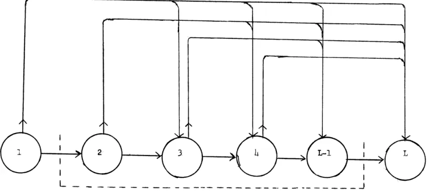
We consider a production process consisting of an L-2 stage production line and stages 1 and L external to the line representing fictitious input and output activities. Potential inspection points exist after each produc-tion stage and will henceforth be identified with the manufacturing stage immediately preceding (Figure 1). Each stage
j
in the production line can generate typej
repairable and typej
non-repairable defects.The following assumptions will be made:
1) A unit with at least one non-repairable defect will be considered a non-repairable item.
2) A unit with any number of repairable defects and with no non-repairable defects will be considered a non-repairable item. 3) After discovery of defects, repairable units are repaired and
returned to the line at the point of inspection, and non-repair-able units are removed from the manufacturing system.
-17
-1
'.4 0 4) 02 fr. Co p4Il
Figure
1
Sequential
Production
Process
I_ 18 _
4) Inspectors are perfect; defects are never overlooked.
5) Inspectors test for all defect types after the previous inspection point. An inspector at stage n thus inspects for defect types in the set (m+l, m+2, . .n), given that the previous inspection point is at stage m.
Initially a lot size, B1, is assigned to the system, where B. is taken
to be the expected number of items leaving manufacturing stage
j
that are either perfect or repairable. Because of assumption (3), then, if there is an inspector assigned to stage k, there would be Bk items eventually leaving the stage to continue in the manufacturing process, and all units would be defect-free.We assume that each stage generates defects independently of every other stage, and that the defect-generating process at each stage is multinomial with stationary parameters pr and pn. Thus, the mass function for e., the
J
event occurring as an operation is performed on an item passing through stage
j
is:pr., e.1 = a repairable type-j defect is imparted to
F
3 the itemf(e ) = pn., e = a non-repairable type-j defect is imparted to the item
1-pn.-pr., e = the operation is successfully executed J J J
An item leaving stage h which was last inspected at stage g may thus have any combination of properties ejk for g < j < h, k = 1,2,3.
Network Formulations
At this point we will look ahead to the shortest-route model formulation in order to make clear the sort of information that will be needed in order to
~19~
solve for an optimal inspection policy. We will compute the set of expected costs, c.., which represent the incremental cost incurred by having an in-spection point at stage
j
of the manufacturing line given that the last in-spection point is at stage i. Clearly, the cost of inin-spection at any stage j is a function of i. We thus seek a value for all c.., j=2,3...L, i < j.Let C =14c..
Once C is known an optimal inspection policy can be obtained with the help of the Lindsay and Bishop theorem. Since any optimal inspection policy will specify either zero or 100% inspection at each potential inspection
point, we must select from the set of all potential inspection points, K, the subset, kcK, at which items will be inspected 100%, and kcfK at which no inspection will take place, which will minimize the total expected cost. Equivalently, an inspection policy in this model can be defined as an L-2 component Boolean vector (62, 63, 6L-1)
n wc if no inspection occurs at stage
j
in which 6
J if inspection occurs at j
Model I
A shortest-route solution to the directed network shown in Figure 2 will give the minimal cost inspection policy desired if there are no
limita-tions on the number of inspection points allowed. Here, c.. represents theij arc length from node i to node
j.
Upon solution for the shortest (lowest cost) route from node 1 to node L,6.=1
if nodej
lies on the shortest path; 6.=0 otherwise. Nodes 1 and L serve a pedagogical purpose only; they provide a common origin and end for the network route.23
~ 21 ~
Model II
If there is a limited number, n, of inspectors available for assignment to the L-2 potential inspection points, a multi-level shortest-route network of the form shown in Figures 3Uand 3b can be solved for the optimal inspec-tion policy. In this network there are n node "levels" plus the origin and end nodes, corresponding to the assignment of at most n inspectors to the potential inspection points. For those nodes on each level which lie on the
k
shortest path from node (1,1) to node (n+2, L) 6 = 1, where
j
is the stageJ
k
and k is the inspector number assigned to the stage plus one. 6 = 0 for J
k
all other nodes in the network and, necessarily 6. must be zero for all k
j
k. Ifd
is defined to be the L-2 component Boolean vectork k k
(62, 63 .... -) for all levels k, then the optimal inspection policy is 2 3 L- 1
* n+l k
given by 6 = E 6 In this network each arc (x,y), (z,w) is assigned
- k=2
-cost c from C.
yw =
Cost Structure
We will now formulate the classes of costs which comprise each cm, mn n=2..L, m=l..n-1.
A. Expected Cost of Scrappage: n
ees = Z cp.(B -B. ) + cd (B -B ) n=2..L-1, m=1..n-1. mn
j=m+2
j
mJ- nmnThis formulation is identical to White's. B. has been defined previously to be the expected number of good or repairable items leaving stage
j
from anj
initial batch size of B . Thus, B =B 1H (1 - pn.) j=2... L-l. The second
1
J
1.ii=2
component of ecs above represents the salvage value from disposal of non-repairable unfinished items, where cd is the market value (or cost of
dis-n
23
3
Figure 34 Mn+2
Figure 3a Model II General Network Form
Network for 2-Inspector, 3-Stage Line
Number of Inspection Points Constrained to be Two or Fewer Figure 3b
~24
-the value of cd might also depend on m, as suggested by White, -the data collection difficulties would mitigate towards keeping this term as simple as possible.
The first component of the expected cost of scrappage above represents the wasted cost of processing items which already have acquired a non-repair-able defect. With cp. representing the cost of processing an item at stage
n j, the processing cost of units ruined at stage i is (B. B cp..
-1ij=i+1l
Hence, the total expected processing loss between stages m and n is
n-l n n-l n
Z [(B -B.) E cp.] or E E (B -B
)
cp.. Upon reversingi=m+1 j=i+1 i=m+1
j=i+1
the order of summation we obtain: n j-1 E E cp.(B -B.) j=m+2 i=m+l n j-1 = E cp. Z (B -B.) j=m+2 3 i=m+l n = E cp (B -B +B -B +B ...+B. -B.
)
.m+2j
m m+1 m+1 m+2 m+2 3- 2 3-1 j=m+2 n = E cp. (B -B. ) j=m+2B. Expected Repair Cost:
n n
erc = B [ E cr.pr.] H (1-pn.)
mn m i=m+l j=m+l n=2... .L-1, m=l..n-1,
- 25
-The probability that there will be a repairable defect of type i and no non-repairable defects of type j, m < j < n is:
n
pr. HI (1-pn.). j=m+l
Hence, the expected cost of repairing type i defects for B units is: m
n
B cr. pr. H (1-pn.) m 1 i
j=m+l
Then the expected repair cost for all possible repairable defect types i between m and n is:
n n Z (B cr. pr. I (1-pn.)) i=m+l m 1 1 j=m+l n n = B
(
Z cr. pr.)(
H (1-pn.)) m i=m+l j=m+1Note that in general the cost of repair of a defect of type
j
is dependent also on the stage n at which it is discovered. Substituting cr. for cr.ini
above does not affect the mechanics of calculation of erc in any way and is thus entirely feasible. In the working model to follow, however, the simpler form was chosen to make easier the task of data entry.
C. Expected Cost of Undetected Defects:
This is one of the most important categories of cost in the present model, the undesirable consequences of outputting defective products being the raison d'etre for quality assurance efforts. These costs may also be the most difficult to ascertain in any actual situation. Included may be the cost of handling and repairing returned items, the loss of company good-will, and the deterioration of dealer loyalty.
-26
-In this model two very simple formulations are given. The first assumes that the cost of undetected defects of different types are additive. In this case the expected cost of undetected defects is
L-1 ecul =B E mL m =m+l = 0 (pn. + pr.) cul. J J J m = 1...L-2 m = L-1
where cul. is the cost associated with a type
j
defect leaving the plant. JIf we assume a fixed penalty cost for a unit with any defect type or combination of defects leaving the plant, then
L-i
ecu2 = B cu2 [1 - (1 - O (pr. + pn.))]
mL m j=m+l
=0
cu2 is the penalty cost for outputting a defective two expressions will give us the arc cost from any end node, L, signifying that inspection last takes
m = 1..L-2
m = L-1
item. Either of node, m, to the place at stage m.
D. Expected Inspection Cost:
White's model contains expressions for the fixed cost of an inspection station plus the per-unit inspection cost at the station. However, it is not at all clear how these costs may be derived. One strategy is to assume that the expected variable inspection cost from inspecting at stage n given that inspection last took place at stage m is a function of both the set of defect types to be tested or inspected for the efficiency of inspection as
where these dummy
- 27
-determined by the order in which inspection takes place. Knowledge of m and n alone uniquely determines the set, S, of defect types to be inspected over at stage n. Thus, S =
(j
/ m <j
< n). We now seek a least-expected-cost inspection sequence over S.The assumptions about the inspection procedure to be used can be sum-marized as follows:
1. There is a unit cost, C., associated with each defect type that is tested for.
2. The inspector inspects or tests for defects in the set S according to some predetermined least-expected-cost sequence
Q
for all items.3. As soon as the first non-repairable defect of any type is discovered (if any), inspection ceases for that item, it is put aside, and the inspection sequence begins anew for the next item.
Thus, the unit expected inspection cost, uic, for any sequential ordering,
Q,
of the elements in S is:uic(Q) = C1 + (1-pn )C2 + (1-pnl) (1-pn2) 3 + .... + (1-pnl) (1-pn2 (1-pnk-1) Ck
Where there are k elements in S and
C. = the unit inspection cost for the defect type inspected for in 1
sequential position i of
Q.
We seek the permutation,
Q
, of the elements of S which, when used as a sequential inspection order, will minimize uic .F
28-Price5 has identified this problem and offered the suggestion that an optimal sequence can be obtained through complete combinatorial enumeration. Thus, if there are k elements in S, k! orderings must be generated, and uic(Q) computed for each in order to identify the optimal sequence. This is clearly a computationally undesirable approach to solution of a problem which arises
(L-2)(L-1) .6
2 times in the inspection allocation model. Derman has investi-gated this problem and discovered a simple rule which will give the optimal inspection sequence for an inspection sequencing problem of which this is a special case. Johnson has considered an inspection situation under rather
different inspection and repair assumptions, but the logical arguments used are equally applicable in this case.
Theorem:
C. Number the k defect types in S according to increasing value of --.
pn. This is the optimal order of inspection.
Proof:
Let
Q'
be the sequenceQ
after interchanging components i and i+1 where i+l < k. Then we have:i-1 uic(Q')-uic(Q) = ( H (1-pn.)) ((Ci+l-pni)C )-(C +(1-pn )C j=1 i+l ii -
Y(pn
Ci+1 -pn C ) positive C. < C+1 which is 0 according as - - , negative pn >pi+a transitive relation. If we successively interchange consecutive components wherever this difference is negative, we are thus led to the rule that
- 29
-C. C. pn. pn.
1J
If the optimal inspection sequence is
Q*,
the total inspection cost associated with inspection at n given that inspection last takes place at m is:*
eiz = B uic(Q
)
+ fic , n=2...L-1, m=l..n-lmn m mn n
where fic is the cost of locating an inspection station at stage n inde-n
pendent of the testing actually done (i.e. a fixed cost).
As an aside, it should be fairly evident that for potential inspection points at any numbered stages a < b < .
uic* < uic* + uic* +...+uic* .
az - ab bc yz
The cost matrix C can be derived from the above cost classes as follows:
c = eic + erc + ecs n=2...L-1, m=l... n-l
mn mn mn mn
cmL = eculML
m=. ... L-l. or ecu2 b
Network Solution
It is well-known that the directed shortest-route problem can be visualized as a transhipment problem in which there is an excess of one unit at the source node, a deficit of one unit at the sink node, and intermediate nodes have
neither deficit nor excess units. The object is thus to transport the unit from source to sink at minimum cost. The mathematical problem is:
rn-i minimize x = Z Z 1=1 jER s.t. x.. = 1 x. - E Sik E -X.m im XkJ = o k = 2,3...m-1 = -1 2 x = x iJ IJ 3 VL
i,j
Since x. . represents the "quantity shipped" from node i to node
j,
x. .=113 IJ
indicates that path (i-j) lies on the lowest-cost route, while x .=0 indicates
iJ
that path (i-j) is not a part of the lowest-cost route. Rk represents the set of nodes immediately following node k, while Sk represents the set of nodes immediately preceding node k. For example, in Model I Rk=(j / j>k),
Sk = (i / i<k), and m=L.
The dual to the transhipment problem above is: maximize yo = yi - ym
s.t. y - y < c Vi, -V jy
y unconstrained in sign
In Model I V. is thus (j / j>i). Y is arbitrarily set to 0.
Ford8 has devised an extremely fast algorithm for solving the dual problem above, exploiting the fact that each row contains but two variables:
- 30 -c.. x.. 13 13 i
Z
j
~R
je R E iE Sk E isS m- 31
-..Assign initially yo = 0 and yi = o for i j 0. Scan the network for a pair i and
j
with the property that yi - yj > c-i. For this pair re-place yi by yj + Cji. Continue this process. Eventually no such pairs can be found, and ym is now minimal and represents the minimal dis-tance from 0 to m...A dynamic programming approach to the problem above is similar, requiring only an ordering of the rows in Ford's algorithm so that only one scan of the inequality set is necessary.
From the Duality Theorem we know that x* = y* = -y. Thus, a solution
0 o m
to the maximization problem above will give the value of the minimum-cost allocation of inspectors in the inspection model. From the complementary slackness properties of the primal and dual problems (see Dantzig
)
it follows that for each row in the dual that is an equality, y. - y. = c..,J l 1
* *
the corresponding primal variable, x.., is > 0. x.. must equal 0 for all
1J -- iJ
other i,j pairs. If we set each of the x..'s in the first group equal to 1, a spanning tree for the network will result, indicating the least-cost route from the origin node to every node in the network. Note that this is not a solution to the primal problem, since we will have included more paths than are necessary to traverse the network from origin to terminal nodes. However, the unbroken route from the initial to the terminal node can now be easily identified, the associated variables of which comprise a solution to the primal problem.
Flexibility of the Model
The model presented is quite flexible in its ability to cope with
multiple kinds of defects occurring at each stage. The partition of defects into repairable and non-repairable classes has already been discussed. In an
-32
-actual industrial situation, however, one stage of a manufacturing process (one operation) may generate more than one kind of repairable or non-repair-able defect. For example, adding a component to an assembly may result in a faulty mechanical connection or a poor electrical connection or both. Dif-ferent costs of repair may arise from these two defect kinds. In the case in which variable inspection cost for defect type
j
is constant regardless of the number of kinds (both repairable and non-repairable) of typej
defects which may occur, the analysis is straightforward. For k repairable typej
defects possible and 1 non-repairable type
j
defects possible let 1pn.= 1 - H (1-pn..) i=J
where pn.. is the probability of an item acquiring a type j repairable defect. J1
Similarly, let
k
pr. = 1 - H (1-pr..). i=l
Consequently, we may take as the repair cost of type
j
repairable defects (which are now of several kinds) the expected cost of typej
defects over the k kinds: k X cr.. pr.. i=1l cr. = J k E pr.. i=1lwhere cr.. is the cost of repairing type
j
repairable defects of kind orJl-severity i. Note that under the assumptions of the model multiple defect kinds affect only pn., pr., and cr.. All cost functions are then based on
J J J
- 33
-List of Variables
B. = the expected number of good or repairable items leaving stage
j.
JC. = per-unit variable inspection cost for type
j
defects. C = matrix of cost coefficients //cmnmnc = incremental cost of having inspection at stage n given that in-spection last takes place at stage m =
dl
in programs.mn
cd = disposal cost (or salvage value) of defective items removed at stage
j.
cp. = unit processing cost at stage
j.
Jcr. = unit repair cost of type
j
repairable defect. Jcul. = cost of a type
j
defect outputted. Jcu2 = cost of a defective unit outputted.
ecs mn= expected cost of scrappage component of can
eic
mn=
expected cost of inspection component of cmn erc = expected repair cost component of c .ecul = expected cost of undetected defects assuming additive costs compon-end of c
mn
ecu2 = expected cost of undetected defects assuming constant costs compon-ent of c
mn
fic. = fixed cost of inspection at stage
j.
L =
#
of stages in model = # of actual production stages plus two. NSPECT = maximum # of inspection locations (in SHORT2).pn. = probability of a unit acquiring a type
j
non-repairable defect. Jpr. = probability of a unit acquiring a type
j
repairable defect. JCHAPTER III
PROGRAMMED IMPLEMENTATION
Computational Requirements
A programmed computational system for obtaining an optimum solution to the inspection problem modeled in Chapter Two is to be described here. A set of ten free-standing computer programs perform the necessary calculations. The basic requirements for this program set are as follows:
1) Efficient computation of arc costs and evaluation of networks for solutions to unconstrained, constrained, and arbitrary policy cost problems. It is desired further to be able to accomodate problems involving a large enough number of stages to discern patterns in inspection station placement in subsequent data runs.
2) Provision of problem solutions with a maximum of flexibility. For example, a convenient method for entering data vectors is desired. In addition, a minimum of recalculation should be required for changes in the data set, within the
limita-tions of programming effort available.
3) Need for a minimum of human solution effort once data has been put into machine readable form. Since the evaluation of the
unconstrained, constrained, and arbitrary policy problems will usually be required of each data set, task initiation
should be as simple as possible.
-- 35
-Programs, Data Files
The ten calculation routines are free-standing programs written in the Fortran IV language and are stored in the user's allotted filestorage area on the main disc of the M.I.T. CTTS time-sharing computer facility (Computa-tion Center). Time-sharing provides much of the flexibility and ease of human intervention desired of this problem-solving system. The user, com-municating on-line with the IBM 7094 computer via a typewriter-like console, can enter, compile, and select programs for execution, as well as establish data storage files. Cost and parameter data are initially entered on
pseudo-tapes (actually one or more disc records) via the console in the form of strings of numbers. The file structure employed is illustrated in Figure 4. CTTS allows the user to load and run object programs utiliz-ing either pre-stored data or data entered from the console at execution times. Each program in this set, as it proceeds, reads the data it
re-quires from the pseudo-tape files and assigns these values to the appropriate variables. In some of the programs presented herein, requests for additional information are printed on the console to elicit the user's reply. The pro-grams are:
1) MASTER. This program will calculate B , m=l... L-1, the ex-pected number of good or repairable units leaving stage m. An assumed initial batch size of 1000 units provides good scaling for all of the calculations.
2) EIC. Expected inspection cost, eicmn, is calculated for all feasible arcs.
3) ERC. Expected repair cost, ercmn, is calculated for all feasible arcs.
-
36-4) ECS. Expected cost of scrappage, ecsmn, is calculated for all feasible arcs.
5) ECU1. Expected cost of undetected defects under the addi-tive cost assumption, eculmL, is calculated for m=l..L-l. 6) ECU2. Expected cost of undetected defects under the
con-stant cost assumption, ecu2mL, is calculated for m=1... L-l. 7) AGGREG. This program will aggregate the components of arc
costs, eic, erc, ecs, and either ecul or e:Ci2 to yield the arc cost matrix C. A message is printed on the console ask-ing the user whether he wants to employ additive or constant costs of undetected defects. The user's response selects either ecul or ecu2 to provide cmL, m=1..L-l.
8) SHORT. This program will evaluate the shortest-route net-work corresponding to the unconstrained inspection problem,
using as input the values of C stored on an intermediate data pseudo-tape. This program will print the minimum total cost
of the optimal policy obtained and the locations at which in-spection stations should be placed. In addition, the minimum arc costs from node 1 to all other nodes (the spanning tree) are listed for further analysis.
9) SHORT2. This program will find the optimal inspection policy for the constrained inspection problem. The user is asked to enter on the console only the maximum number of inspection stations to be allowed. All other work, including building up the extended network of feasible arcs and assigning arc costs, is done by the program. The console will print the optimal location of inspection stations and the total quality cost of the policy.
- 37
-10) LONG. This program will evaluate the total quality cost of any arbitrary inspection policy. The user is asked only to enter on the console the numbers of the stages at which inspection is to take place. The program will then print on the console the total cost of the policy entered.
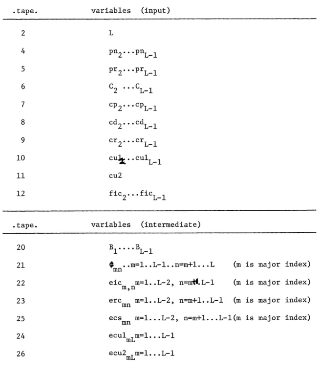
Each program above will read in the required data from the appropriate pseudo-tapes and output data onto the appropriate intermediate files as shown in Figure 4. More detailed descriptions of these programs and statement list-ings may be found in the appendix.
- 38
-FIGURE 4 FILE STRUCTURE
Input and intermediate variables stored in pseudo-tapes (one or more disc records)
.tape. variables (input)
2 L 4 pn 2...pnL-1 5 pr 2... prL-1 6 C2 ... CLL-1 7 cp 2... cPL-1 8 cd 2..cdL-1 9 cr2...crL-1 10 cuI. cul L 11 cu2 12 fic 2..fic
.tape. variables (intermediate)
20 B ....
BL-1
21 $ ..m=1..L-l..n=m+l...L (m is major index) mn
22 eic m=l..L-2, n=mi.L-1 (m is major index) m,n
23 erc m1. .L-2, n=m+l..L-1 (m is major index) 25 ecs m=...L-2, n=m+l...L-l(m is major index)
24 ecul m=1... L-1
mL
- 39
-Execution Sequence
Input data must be entered in the proper pseudo-tape files before any calculation can take place. Each object program may be loaded and executed under CTTS through the use of one or two simple commands communicated via
the console.
Starting with new data, the complete solution requires the execution of several programs in sequence, as illustrated in the flow chart of Figure 5. First, MASTER must be executed to provide the vector B which is utilized as input to the arc cost component programs. Next, EIC, ERC, and ECS are executed in any order to provide arc-cost components. ECUl or ECU2 or both must also be executed at this time to provide cmL, m=1...L-1, although only one of these data sets will be used in aggregation. AGGREG is next executed to aggregate erc, eic, and ecs, providing arc costs, and either ecul or ecu2 provides terminal arc costs. The program requests the user to indicate on the console whether he desires the additive or constant cost formulation of expected undetected defect costs.
Once the arc-length matric, C, has been outputted, one or more of the network routines, SHORT, SHORT2, or LONG, may be executed to yield policies and total quality costs. In addition, if only some data entries on pseudo-tapes are revised, only the programs to do the affected calculations need be re-executed. Only if the pr or pn vectors are changed must the full
sequence of programs be rerun, as all arc cost components include elements of the vector B.
'U -40
-figure
5
I-
- - -- - -
-I ENTER DATA ON
Executibt-ha
Sequence
PSEUDO-TAPES
L
RUN SHORT unconstrained solutionRUN SHORT2
constrained
solution
RUN LONG arbitrary policy cost RUN MASTERRUN EIC, ERC, AND ECS
I
I
-41
-Choice of Solution Structure
Separate programs for arc-cost calculation were adopted to permit re-execution of fewer than all of the programs if data elements of one or two types only are altered. This has already been mentioned. The use of a con-trol program which would execute several or all of the programs described above as subroutines was considered, but this idea was discarded since it would require at least as much user effort in task specification as is pre-sently required in executing the free-standing programs in sequence. The use of pseudo-tape files for storage of input data permits data entry via the console prior to program execution at the user's convenience and rapid read-in of data from files (disc records) to core as each program is executed. As mentioned earlier, the input data sets are limited to vectors for ease of manual data entry, although some data element types may be considered to be matrices in the general mathematical model (unit repair costs, for example).
Storage of the elements of the arc-cost matrix C on intermediate pseudo-tapes permits the evaluation of constrained optimal, unconstrained optimal, and arbitrary policies utilizing the same set of final arc-cost data. Thus, the effects of constrained inspection resources of various degrees and ex-isting policies can be readily compared without additional arithmetic calcu-lations.
Computational Experience
There appear to be no major computational difficulties associated with the inspection model. Calculation of arc costs is straightforward as des-cribed, although perhaps unsparing of computer time for problems of greater size than those considered here. This remains to be seen. The following total computation times are typical for lines of the length indicated.
~42
-L = # of stages (including initial and terminal) Total Time
5 47.93 sec
12 52.28
22 63.05
50 134.13
These data are plotted in Figure 6. We cannot, however, place much emphasis on the reproductibility of these figures since (1) total time includes on the average 20% swap time, which may vary from run to run with the same data and program, and (2) total time includes program and data file retrival and program load time of a setup nature.
Also, since the number of calculations required for the 5-stage (3 physi-cal stages) problem is quite small we may assume that virtually all of the 47+ seconds required for solution to this problem is of a setup nature and represents a fixed cost of using separate programs and the file search time of the time-sharing system.
It is interesting to note, however, that the number of arcs for which cost components must be calculated is approximately equal to S- , where s is the number of stages in the system, and that the average arc-cost compon-ent calculation is roughly proportional to the number of stages that the arc spans. We might then expect a priori that an approximately cubic relation-ship exists between arc-cost calculation times and the number of production stages. Moreover, approximately
--
calculations are required for the un-constrained network solution, MASTERjand AGGREG. Therefore, total problem solution times should increase initially somewhat less rapidly than the cubetime to compute
(seconds)
S I I * I10
Figure
6
Computation Time
150-- 43
-100
4
50
-0
20
30
40
50
a
- h
-
44-of the number 44-of stages, but more rapidly than the square. This is sug-gested also by the curve on Figure 6 which increases less rapidly than a function of a cubic term only, but more rapidly than that of a square term
2 3
only. The total time function might then be of the form c+as +bs3. For lines of many stages we would expect the cubic term to dominate, rapidly limiting the maximum problem size that can be economically handled. Further empirical investigations with larger problems would be necessary in order to validate the hypothesized computation time relation. These were not attempted
in the present investigation due primarily to the inability of SHORT2 to
build up feasible arc identification vectors for problems significantly larger than the ones tested without approaching the 32k user available core capacity of CTSS.
Computational Limitations
The program set employed in this investigation is designed to allow maximum flexibility for experimentation and evaluation of parameter structure on inspection policies. No effort has been made either to minimize computa-tion times or to solve problems of the largest size. It is likely that the elimination of separate free-standing programs for different solution steps would significantly reduce the program find-and-load time of 47+ seconds. Batch processing with a more powerful machine than the 7094 and more effici-ent programming might also significantly reduce solution time. However, the cubic relationship between line length and total solution time must still be reckoned with.
In an implementation designed specifically to handle large problems arc-cost components might be aggregated as calculated, to eliminate the loading
- 45
-of three matrices and one vector into core to be aggregated into the matrix of arc costs, C. Thus matrices with three times as many elements may be handled with the same core capacity as with the present set-up. A machine with a large fast core storage area available to the user (on the order of
150k data words) should, with proper programming, be able to provide at least optimal unconstrained solutions for problems of about 300 stages if the entire arc cost matrix is loaded into core prior to network calculations. This is not at all a requirement, however, since the unconstrained and con-strained network algorithms can utilize parts of this cost matrix at a time to evaluate minimum-cost routes from the initial node to all other nodes work-ing sequentially from lower-order nodes to higher-order ones, savwork-ing only the minimum cost to each node already evaluated. Thus, in theory and with relat-ively little change in the SHORT and SHORT2 programs the solution to problems of much larger size than 300 stages is potentially feasible if, in addition, arc-length component costs are removed to supplementary storage periodically as they are calculated by the arc-cost routine and accumulate.
Perhaps more significant than the feasibility and economics of calcula-tion for large problems is the data-gathering effort required. It is, for example, unlikely that the probabilities associated with the defect-generat-ing processes at each stage will be immediately available, unless records of defect repair have been kept in the past. A study may thus have to be undertaken, in which there would in many instances be a high likelihood of data contamination resulting from attention focused on the production line. In addition, cost components such as repair costs and penalty costs for un-detected defects may be non-standard or measurable. Thus, collection of both the quantity and the types of data necessary in order to implement this
CHAPTER IV
EXPERIMENTAL RESULTS AND ANALYSIS
This chapter contains the results of several runs made with the computa-tional system described in Chapter III. For the first input data set employed, the behavior of total quality cost with various inspection policies is
analyzed. Next, the effects of parameter values on optimal solutions is dis-cussed. The third section of this chapter is concerned with the change in optimal inspection policies arising from a different processing cost structure than in the first data set. In the last section the relationships between fixed inspection costs, total quality cost, and optimal policies are examined.
Data Set I - Example
The first set of data to be employed in the model is the following: L = 50 (48 physical stages) pn. = .02, j = 2.. .49 J pr. = .05,
j
= 2...49 J C. = .025,j = 2.. .49 J cp. = .20, j = 2.. .49 cd. =-.05j,j = 2.. .49 J cr. = 2., j = 2...49cu2 = 20 (constant undetected defect cost formulation)
These figures have been chosen to be typical of what might be found in an assembly-line process consisting of many small operations. The electronics industry provides many good examples. To simplify the analysis which follows, stages were assumed to be identical in associated costs and in defect-generat-ing frequencies.
-
-47-COMPUTATIONAL RESULTS - DATA SET I
Number Of Inspection Points Stages TQC
0 19385.939 1 (optimal constrained) 49 4548.006 2 (optimal constrained) 23,49 3774.942 3 (optimal constrained) 15,31,49 3619.872 4 (optimal) 11,22,35,49 3580.167 5 9,18,28,38,49 3580.456 6 7,14,22,31,40,49 3599.244 6a 8,16,24,32,40,49 3599.415 6b 9,17,25,33,41,49 3601.113 6c 9,16,23,34,40,49 3601.996 7 6,12,19,26,33,41,49 3627.288 7a 7,14,21,28,35,42,49 3628.197 8 6,12,18,24,30,36,42,49 3661.669 9 6,11,16,21,26,32,38,42,49 3700.621 9a 5,10,15,20,26,32,38,42,49 3700.691 10 5,9,14,19,24,29,34,39,44,49 3740.068 ---DATA SET II 2 (optimal constrained) 26,49 12442.688 3 (optimal constrained) 19,34,49 8666.929 18 (optimal) 6,10,13,16,19,22,25,28,31, 4550.824 33,35,37,39,41,43,45,47,49
-48-Total
Quality
Cost
4500
4400
4300
4200
4100
4000
3900
3800
3700
3600
1
2
3
4
5
Figure
7
6
7
8
9
10
Inspection Points
Data Set I Total Cost Curve
A--4 * I r '*'---
'
---
7
-49
-The cost of disposal is negative, indicating a positive salvage value of non-repairable units in various states of completion. The salvage value rises linearly with the number of operations having been performed on the unit (if each operation is the addition of a component to an assembly this may be a fairly good approximation). Thus, a non-repairable unit removed from the process at any point will have approximately one-fourth of its cumulative processing cost recovered when scrapped.
The optimal unconstrained, constrained, and arbitrary policies are tabulated on the next page with the total quality cost (TQC) for each case considered. The optimal number of inspection stations was found to be four, distributed very nearly evenly among the 48 stages, with slightly increasing spacing near the end. Total quality cost for this policy is $3,580.17 for a batch size of 1000. Even as the maximum number of inspection points is constrained to various degrees, the inspection stations continue to be dis-tributed more or less evenly for minimum TQC, as the total cost of course rises. This suggests that an intelligent choice of policies for an arbit-rary allocation of more than the unconstrained optimal number (four) of in-spection points might be to distribute these stations approximately uniformly. This was done for policies utilizing 5,6,7,8,9, and 10 stations.
Two significant insights can be gleaned from the computational results. The first of these is derived from the behavior of total quality costs as the number of inspection stations is varied. Of course, a very high TQC results from no inspection at all due to the imputed cost of outputting defective units. This cost is equal to cu2 times the expected number of units with a
L-1
defect of at least one type, B (1 - II (1-pn.+pr.)). The cost of $20 for
1 j=2
'
each defective unit outputted ensures, given the other data, that an optimal policy will require that inspection take place at the last stage.