A Comprehensive Electromagnetic Analysis of AC
Losses in Large Superconducting Cables
by
Yu Ju Chen
S.B., Massachusetts Institute of Technology (1990)
S.M., Massachusetts Institute of Technology (1990)
Submitted to the Department of Electrical Engineering and Computer
Science
in partial fulfillment of the requirements for the degree of
Doctor of Philosophy in Electrical Engineering
at the
MASSACHUSETTS INSTITUTE OF TECHNOLOGY
September 1996
@
Massachusetts Institute of Technology 1996. All rights reserved.
Author ..
Departn~nt of Ele4ical Engineering and Computer Science
September 4, 1996
Certified by...
effrey P.rofeidberg
Professor
Thesis Supervisor
n,
Accepted by ...
if
v v..
v .vw ~. ...Frederic R. Morgenthaler
Chairman, Depart ental Co mittee on Graduate Students
OCT 15 1996
Large Superconducting Cables
by
Yu Ju Chen
Submitted to the Department of Electrical Engineering and Computer Science on September 4, 1996, in partial fulfillment of the
requirements for the degree of
Doctor of Philosophy in Electrical Engineering
Abstract
The issue of AC losses in full-size superconducting cables has been explored both theoretically and computationally in this thesis. A substantially accurate model is presented which captures the dominant physical behavior of a composite supercon-ductor, whether it be a single multifilamentary strand or a large cable.
A set of analytic solutions, the first of its kind available, has been derived for a wide range of geometries. In the process, there is a formal proof that twisting filaments or strands reduce losses. The effect of cable terminations on current distribution and loss has been outlined and a criterion is given for determining the regions of validity for the infinite cable assumption. This assumption, in turn, lays the foundation for the implementation of the computational part of the thesis.
A nonlinear 2D computer program, which takes into the effect of superconducting saturation, has been developed and implemented. As a result, current distribution and loss profiles of a multifilamentary strand can be solved with great accuracy and efficiency, thereby adding new capabilities in the analysis of losses in multifilamentary strands.
A 3D code, tailored to the geometry of the proposed ITER cable-in-conduit con-ductor (CICC), is the final contribution of this thesis. The need to accurately describe the geometry of the CICC lead to the cable winder algorithm. From the derived strand trajectories, the 3D code produces current distributions and losses for transverse mag-netic fields. Loss characteristics were compared against available experimental data. A new set of results and design recommendations emerged from the analysis.
Thesis Supervisor: Jeffrey P. Freidberg Title: Professor
Acknowledgments
I would like to thank Prof. Jeff Freidberg, for which this thesis would not have been possible without his guidance and support.
I would also like to thank Prof. Richard Thornton and Dr. Bruce Montgomery for providing me with the opportunity to work on superconducting magnets. I con-sider myself fortunate for having been able to work on interesting projects such as MAGLEV and fusion.
Thanks go to Prof. Jacob White for taking time out of his busy schedule to be one of my thesis readers.
Throughout my years at MIT, I have made some great friends. Kudos go to Grundy for helping me out with some of the figures in this thesis. I am also grateful to my good friend up north, Alain (sheema) for some fruiftful technical discussions. And there is, of course, the people I befriended at Ashdown: my original dorm-mates, Karin and Anne, and of course my Athena buddy, JP, who followed me home after my PWE's. Gratitudes to my sisters-in-arms, Meechoo, Sue, Steph, for all those female-bonding sessions. I also have to thank Matt and Shiufun for all the times they
put up with me being in their suite - all those TV nights have finally paid off! Finally,
I want to thank my friends from undergraduate (Andrew, Jo, Wendy, Ting, Illy, Suz, etc.) for being such good friends during my undergraduate years here. Special thanks go to Lisa for being such a wonderful supportive friend and for always being there to share my experiences with me.
Last, but not least, I want to thank my parents for making me who I am - to my
father who sparked my interest in the sciences and to my mother who always had faith and was always there to take care of me.
Contents
1 Introduction to AC losses
1.1 Loss mechanisms in superconductors . . . . 1.2 Literature Survey ...
1.3 Scope of the thesis ... 2 The Model
2.1 Field Distribution in Magnet Windings . . . .
2.1.1 Solenoids ...
2.1.2 Toroids ...
2.2 Ordering system ... 2.3 Governing equations ... 2.4 Constitutive relations. . . ...
2.5 Formulation of Boundary Conditions . . . . .
2.5.1 Magnet connected to a current source .
2.5.2 Magnet in persistent mode . . . .
2.6 Conclusion ...
3 Analytic Results of Limiting Cases
3.1 Open-circuited straight cable ...
3.2 Short-circuited current loop ...
3.2.1 Untwisted wires ...
3.2.2 Twisted wires ...
3.3 Finite length twisted cable ...
13 16 17 20 25 . . . . . 26 . . . . 26 . . . . 27 . . . . 27 . . . . 29 . . . . 32 . . . . . 34 . . . . . 34 . . . . . 45 . . . . 49 51 . . . . 51 . . . . 57 . . . . 57 . . . . 62 . . . . 68
3.3.2 Open-circuited ends ... 70
3.3.3 Short length limit ... 72
3.3.4 Long length limit ... 74
3.4 Conclusion . . . .. . . . .. . 75
4 2D code 83 4.1 Num erics . . . .. . 84
4.2 Benchmark cases ... 90
4.2.1 Case 1: Linear conductivity . ... 91
4.2.2 Case 2: Wire with thin normalconducting shell ... 92
4.2.3 Case 3: Multilayer wire - SSC NbTi strand . ... 93
4.2.4 Case 4: Field ramp with transport current . ... 101
4.3 Conclusion . . .. .. .. .. .. .. .... .. . .... . .. . .... 103
5 3D code 111 5.1 The Cable W inder ... 112
5.1.1 The algorithm ... 112
5.1.2 Results of cable winder ... 118
5.1.3 Analytic model of pC ... 127
5.2 Governing equations for the ITER cable ... 129
5.3 Numerical strategy ... 132
5.4 R esults . . . .. . 140
5.4.1 Field and Loss Profiles ... 148
5.4.2 Loss data . . . .. . . . . 157 5.5 Design Recommendations ... 162 5.6 Conclusion . . . . .. .. .. . .... .... . ... ... .. . .... 166 6 Conclusion 169 6.1 Sum m ary ... ... 169 6.2 Concluding remarks ... 172
List of Figures
1-1 Flux pinning vortices in type II superconductors . ... 13
1-2 Pictures of single strand conductors . ... 14
1-3 Sketch of different types of cables. . ... . 15
2-1 Flux lines in short solenoid magnet. . ... 27
2-2 Definite of coordinate system ... ... 35
2-3 Prototype of ITER joint sample ... 41
2-4 M odel of joint ... 42
2-5 Sketch of persistent loop ... 46
2-6 Model of persistent joint ... 48
3-1 Untwisted finite length cable. ... 52
3-2 Transport current loss for a persistent loop. . ... 78
3-3 Dipole current loss for a persistent loop. . ... 78
3-4 Transverse ac loss currents in single twist pitch cable . ... 79
3-5 Current density for short and open-circuit ended cables ... 80
3-6 Loss for short-ended cable ... 81
3-7 Loss for open-ended cable ... 82
4-1 Schematic of multilayer strand ... ... 104
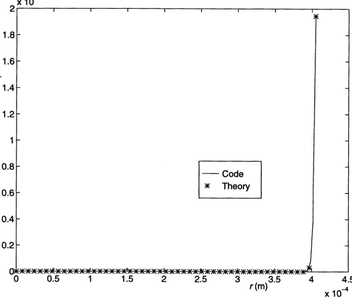
4-2 Ell: comparison of analytic and code-generated results ... . 105
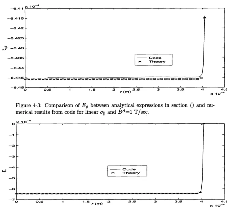
4-3 E4 . . . 106
4-4 E . . . . . 106
4-7 Power loss of NbTi strand in ripple field
4-8 Transport current profile as affected by B
5-1 5-2 5-3 5-4 5-5 5-6 5-7 5-8 5-9 5-10 5-11 5-12 5-13 5-14 5-15 5-16 5-17 5-18 5-19 5-20 5-21 5-22 5-23 5-24 5-25 5-26 . . . . . 109 . . . . . 110
Cross-sectional view of ITER cable . . . . . . Winding process of ITER cable ... Pictorial of cable winder algorithm . . . . Strand locations in a leaflet ... Path of a strand through the cable . . . . P '. .. . . . ... . . . . p in global coordinate ... p4 in global coordinate ... a - the radial profile of p . .. . ... Top view of cable - verification of a . . . . Radial profile of ý . . . . . Comparison of analytic model with data of p Saturated vs. non-saturated power loss for B= Saturated vs. non-saturated power loss for B= Eli and Er profiles without a noise . . . . Illustration of a noise ... Mean-squared noise of a vs. radius of cable.. Cross-sectional profile of Ell . . . . Cross-sectional profile of E ... Cross-sectional profile of Er . . . . Cross-sectional profile of E, ... Cross-sectional profile of power density . . . . pd as function of oal... Pd as function of B ... Pd as function of t ... 154 154 155 . . . . . 112 . . . . 113 . . . . . 117 . . . . 119 . . . . . 120 . . . . 121 . . . . 122 . . . . 123 . . . . 124 . . . . . 126 . . . . . 126 . . . . 128 . . . . . 130 1T/s ... . 141 10T/s . ... 141 . . . . . 144 . . . . 145 . . . . . 147 . . . . 149 . . . . 150 . . . . 151 . . . . 152 . . . . . 153
5-27 Excitation field waveforms for benchmark experiment ... . 159
5-28 Experimental data for sawtooth waveform . ... 160
5-29 Experimental data for sine wave ... .. 161
5-30 Schematic depiction of the interplay between the fourth and fifth stage. 163 5-31 a profile of recommended ITER cable design. . ... 164
5-32 p profile of recommended ITER cable design. . ... 164
5-33 Power loss vs. time for recommended ITER cable design. ... 165
List of Tables
1.1 List of superconducting magnet applications . ... 16
3.1 A table of analytic results for different conductor geometries and end conditions .. . . . .
5.1 Specifications of ITER cable ... 114
Chapter 1
Introduction to AC losses
Since the discovery of the phenomenon of superconductivity in 1911 [1], there has been ongoing research to develop applications to utilize superconducting properties. As a result, there have been many types of materials and engineering products developed. This thesis is concerned with applications which utilize superconductors as large scale conductors.
Naturally occuring elements such as mercury fall into what are termed type I superconductors. These conductors, when cooled below a critical temperature and subjected to a magnetic field less than the critical field, expel flux by means of a very
0000>(
(X)0 0(
0000>(
0000(>
(00)
Figure 1-1: (a) A uniform array of vortex currents produces no net current density but (b) a gradient in the density of vortex currents produces a net current
00
0DC
C,(
Figure 1-2: Several composite conductors: (a) Nb3Sn multifilamentary conductor
(b) NbTi monofilament conductor (c) Classical NbTi conductor (574 fil.) (d) AC conductor(i5k fil.)
thin surface current. This phenomenon is termed the "Meissner" effect. Another class
of bulk superconductors called type II superconductors operate in a "mixed state" by
allowing a much larger magnetic field to penetrate before it becomes normal. This is made possible by the presence of flux pinning vortices. These "fluxoids" produce vortex currents as shown in Fig. 1-1. A gradient on the density of these currents produce a net current inside the conductor, not just on the surface. This is what allows the external magnetic field to penetrate the conductor and result in a much higher critical field. The composite conductors mentioned in this thesis use type II bulk superconductors.
Nb3Sn thin tapes in 1957. In 1963, the first NbTi monofilament strands were
pro-duced. For stability reasons, these monofilament strands became multifilaments em-bedded in a normal conducting metal base (see Fig. 1-2). To reduce losses, the multiple filaments were also twisted.
For large systems, high-current cables were developed. These cables are manu-factured from many multifilamentary strands. The following two types of cables are often used:
a
C-Figure 1-3: (a) 11-strand Rutherford-type cable (b) Cable-in-conduit conductor (c) Cable without a jacket.
* Rutherford cables (see Fig. 1-3(a)) are flat multi-strand cables. Because Lorentz forces can displace strands which in turn can cause quenches, these cables are packed tightly (90% fill fraction).
Application Solenoids NMR Fusion High-energy physics MRI SMES MAGLEV DC motors AC generators Magnetic separation MHD Small bore Large bore Toroidal coil Transformer coil Beam-guiding Detectors Pulsed Low frequency Conductor
W
CW
CIC CIC RC CW
C,RC C,RCW
RC RC C RCTable 1.1: The main characteristics of superconducting magnets. W=wire,
RC=Rutherford-type cable, CIC=cable-in-conduit, C=cable without jacket.
* The cable-in-conduit conductor (CICC) as shown in fig. 1-3(b) is manufactured in several stages, each stage with its own sub-bundles twisted together. An incoloy jacket supports the conductor and contains the liquid helium. The forced flow cooling gives additional heat transfer inside the cable.
The main applications for superconducting magnets are outlined in Table 1.1. In this thesis the emphasis is on the electromagnetic properties of circular multi-strand cables such as the CIC conductor used in fusion machines and on proposed magnetically-levitated (MAGLEV) trains.
1.1
Loss mechanisms in superconductors
When the transport current inside a superconductor and/or the magnetic field it experiences do not vary with time, there is no power loss. This is a primary reason for using superconductors. With a time-varying magnetic field and/or transport
Max. field on conductor [T] 20 15 20 13 13 12 6 0.5-2 5-10 5-10 5 2-5 2-6 8 8 Field-sweep rate
[T/s]
10 -small small 0.1-10 0.1-10 10.2 small 1073 103-104 small 0-10 small 10 small small1.2. LITERATURE SURVEY
current, electric fields are induced and joule heating ensues. These losses demand more refrigeration or in worse cases, they may be the culprit to quenches in the
system. There are three major types of losses - loss due to magnetization in the bulk
superconductor, resistive loss due to coupling currents flowing in the normal metal region of the composite conductor (across the copper matrix inside a strand or strand-strand current via contact conductance), and loss incurred by transport current when it experiences a finite resistance.
Magnetization or hysteretic loss is well-understood and predictable [29][11]. Since these losses occur in the filaments, their magnetization effect is small. The maximum magnetization Mp of a round filament is ~LpoJa where Ja is the critical current
density and a the filament radius. Typical values of J, =1 x 10⁹A/m3 and a = lpm
give MP = 5.33 x 10⁻⁴T, which is negligible.
Therefore, the objective of this thesis is to develop and analyze models which predict the AC losses caused by electric fields and currents flowing macroscopically in and between strands in multistrand CICC. The losses predicted by this model can aid in the design of the refrigeration system, in future cables, or in predicting possible quench mechanisms. The current distributions and time dependence behavior obtained from the model can shed light on ramp-rate limitations of magnets which require fast ramp rates (for instance, the central solenoid of a fusion reactor like ITER).
1.2
Literature Survey
Current redistribution in full-size cables, as applicable to the calculation of AC losses and stability, has not as yet been adequately treated in the literature. Methods vary in sophistication, from one as simple as that used in the ITER coil design guidelines [7]
to a full-scale electromagnetic treatment of the problem as presented in a paper from the University of Twente [10].
It has been experimentally observed that the rate of decay of induced currents inside these superconducting cable is orders of magnitude longer than that of a single strand. It is thus safe to say that the behavior of a cable is a far departure from that of a strand. There are two major differences. First of all, the geometry of a cable is more complicated. The strands not only twist helically but transpose on each other radially. A wire that is skirting the perimeter of the cable at some position along the cable may find itself somewhere near the center or even on the other side further down the length of the cable.
The other major difference is in the ratio of the parallel conductivity to the per-pendicular conductivity. In a strand, when a filament saturates, the current flows at critical current density and any excess current will spill into the next filament or into the copper matrix surrounding it. The perpendicular conductivity is simply equal to some fraction of the conductivity of copper. In other words, in the saturated region(s) of a strand, due to competing conductivities in the parallel and perpendicular direc-tion, large transverse fields and currents are induced. In the case of a cable, when a strand saturates, the remaining current will spill into the normal metal region of the strand or transfer to a neighboring strand via the interstrand conductivity. How-ever, unlike filaments in a strand, the transverse interstrand conductivity is orders of magnitude smaller than for copper. Even in saturation, it is much smaller than the parallel conductivity of the strand. Under these conditions, parallel fields will remain small compared to their transverse counterpart. Even more importantly, because the transverse currents are also small, one sees a much smaller shielding effect than in the single strand. The following section briefly outlines the existing literature which attempt to solve for losses in a complex cable.
1.2. LITERATURE SURVEY
For the proposed ITER coil, the formulae most commonly used to calculate cou-pling loss due to strand-to-strand contact are the same as those used for a single strand. They are simple and fully analytic, and use an experimentally derived time
constant and unknown geometric factor, nT, of the cable. Because it is essentially
only an equation for power dissipation, no insight into the current distribution of the cable can be gleaned from this calculation.
Turck [8] and Ciazynski [2] evaluate the current distribution of two twisted strands. Their model consists entirely of discrete circuit elements. They calculate the self-inductance of the wires, the mutual self-inductance between them, and model the contact resistance with resistors periodically placed along the length of the twisted strands.
From the behavior of two twisted strands, they extrapolate an estimate of the current transfer behavior within the ITER cable.
Several papers from Japan [5] [6] and one by Egorov [3], use the same approach in solving for AC losses caused by interstrand coupling. They all obtain analytical solutions for the voltage induced in each of these strands by a uniform transverse magnetic field. From these voltages, one can find the voltage drop across two adjacent strands to calculate the amount of interstrand coupling current. In [5], they examine three and seven strands twisted together. Egorov treats the interstrand currents for the entire cable with the same method. Similarly in [6], the voltage induced in the
strands are used to calculate interstrand current distibutions. They find, via the finite element method, the current distribution in the normal metal region of the strand which surrounds the filament region.
They were able to obtain an analytical solution for the induced voltages by assum-ing that the electric field along these strands is zero. The magnetic field distribution is assumed to be constant across the cross-section and along the length of the braided strands, i.e. no induced magnetic fields are included in these analyses. Because any
shielding effects are neglected, the field in the structure is equal to the applied field. These assumptions are valid for relatively small or slow field variations. In addition, the limited number of wires in their model makes the assumption of negligible in-duced magnetic fields reasonable. Finally, the complex effect of transport current on current distribution was not fully discussed in either of these papers.
The work from the University of Twente is the first to attempt to solve the
com-plete AC loss and stability problem in full-sized cables [91 [13]. Discrete circuit
equa-tions are used to model the cable. A simple relaequa-tionship between V and I for a single strand is used to capture the nonlinear behavior of the superconducting strands. This
V vs. I relationship is crucial to modelling if and when wires in the cable saturate.
L.J.M. van de Klundert reports that due to the wires' non-linear behavior and strong
dependence on !%B, the solutions are difficult to obtain [9]. A. Verweij [18] recently
published a Ph.D thesis on the analysis of Rutherford cables used in accelerator mag-nets. No definitive electromagnetic model of full-size three dimensional cables have as yet been reported.
The estimates on the AC losses in CICC are contingent on an experimentally derived parameter, the time constant. In order to predict the behavior of a system, one should rely solely on physical parameters to make an estimation. The time constant should be part of a set of results, not the means to a result. In other words, at the present time, there in no direct way to reliably estimate AC losses given the available analytical and numerical tools. This is the prime motivation for the thesis.
1.3
Scope of the thesis
Our model is philosophically most similar to the work done at the University of Twente. The major difference is that our model is spatially continuous and thus
1.3. SCOPE OF THE THESIS
uses E's and J's versus V's and I's. Another difference in modelling arises from the fact that during manufacturing of cables, the substages are compressed to fit through specified die sizes. This results in strands that do not necessarily rotate around fixed radii. Our model can trace through the current paths of each strand in the cable. From the strand trajectories, one can then solve for the field distribution inside the cable.
The next chapter describes the model we use. It lists the assumptions and or-dering system for which the model is based. The oror-dering is based on a long, thin approximation where the geometry and the excitation source vary slowly in z, the ax-ial coordinate of the conductor. The result is a general set of two coupled differentax-ial equations derived from Maxwell's equations with two unknowns: Ell, the magnitude of the electric field parallel to the superconducting portion of the geometry, and 4, the transverse potential. The nonlinear constitutive relationship between all and Ell found in Carr [12] and Rem [4] is used in the governing equations. Boundary condi-tions along the rim and ends of a cylindrical geometry are derived. The model can be applied to a composite conductor of arbitrary geometry, as long as the inner geometry is not too tightly twisted.
In chapter 3, the governing equations and boundary conditions are used to derive analytic results for geometries containing one twist pitch. The tractable solutions are summarized here:
* Infinite length conductor (twisted)
* Infinite length conductor in a closed-loop (twisted)
* Finite length conductor with open ends (untwisted)
* Finite length conductor with shorted ends (twisted)
The analytic results when taken to the appropriate limit match those found in lit-erature. In addition, a constraint on the regime of validity for the infinite cable has been derived. This is important for conducting experiments and for understanding the applicability of theories which use the infinite cable assumption.
Chapter 4 marks the beginning of the computational section of the thesis. With the differential equations, constitutive relations, and boundary conditions derived, a "2D" code was developed and implemented. The purpose of creating this code is to benchmark the model. The code solves for problems in polar coordinates r and q and can be applied to long cables. The numerical strategy for solving the differential equations and for treating the nonlinearity in all is outlined. A number of cases with various geometries have been used for comparison against both analytic solutions from chapter 3 and well-established literature results.
The problem of the CICC cannot be solved simply by the code described in chapter 4 because the inherent geometry of the cable is three-dimensional. Chapter 5 describes a "3D" code which solves for the current distributions and AC losses given the strand trajectories produced by the cable winder program. The results presented in this chapter are quite surprising. Due to the relationship between the last and the second to last stage twist pitch, a "zero-crossing" phenomenon corresponding to an effective untwisting of the cable appears which results in increased and highly localized joule
heating. In addition, a new time constant, T7 was discovered and it is much larger
than the nT value extrapolated from experimental energy loss data. This implies that the geometric factor n is much smaller than that for a helically twisted cable. A long time constant can actually be seen in some preliminary AC loss data for a 192-strand cable which is 1/6th the size of the ITER design cable.
1.3. SCOPE OF THE THESIS
coefficients. These aided in the conceptual design of a new cable which can potentially yield better performance from an AC loss point of view. The loss results of the recommended design closes the final section of the thesis.
Chapter 2
The Model
A cable is usually built of several stages, each stage consisting of several substages of wires twisted together with its corresponding twist pitch. For most large scale applications, these full-size cables contain on the order of a thousand strands. With such a large number of wires, one is motivated to use a macroscopic continuum ap-proach to solve this structure. Instead of treating each wire discretely, one can model the cross-section as a continuous medium, with "locally averaged" parameters and characteristics. This avoids the gruesome task of finding self and mutual inductances and specifying differential equations for each and every one of the one thousand plus strands in the cable.
The continuum model is coupled with an ordering system which implies all
pa-rameters and fields vary slowly with z. This long, thin approximation is applied to
Maxwell's equations. A set of coupled differential equations emerge. These equations
need to be solved in the two variables Ell and D. The geometry of the problem is
encapsulated in the unit vector I1." The conductivity of the superconductor, all, is the
nonlinear portion of the problem and is explained in section 2.4. Finally, boundary conditions for a circularly shaped cable are derived along with end conditions which
arise from cable-joint interface.
2.1
Field Distribution in Magnet Windings
There are several types of superconducting magnets. Each have their unique field profile which is pertinent to the calculation of AC losses. Whole books have been written on the subject of field calculation so here, only the essentials are outlined. There are two important characteristics of the B-fields inside the magnet windings. In most windings, both the static and the pulsed field are perpendicular to the cylindrical conductor. In addition, if the cross-section of the conductor is small enough compared to the total cross-section of the magnet, it is safe to assume the B-field is uniform across the conductor.
2.1.1
Solenoids
The simplest solenoid is that of the infinitely long one. The field everywhere is in the axial direction, is perfectly uniform across the bore, and falls to zero at the outer edge of the winding. Each section will contribute a field within its own bore of
AB = 0 JAr where Ar is the radial thickness of the conductor section. For the nth
layer of conductors in the solenoid, the self-field would be B0 = pronJAr. If n >> 1,
then AB << B0.
In coils of finite length, (pancake-wound or racetrack coils would be the extreme cases), the situation becomes much more complicated because of the way in which field lines curve around the ends of the coil. Fig. 2-1 shows the flux line pattern for a short solenoid, together with contours of constant-field amplitude, normalized to the central field.
2.2. ORDERING SYSTEM
Figure 2-1: Flux lines in short solenoid magnet.
2.1.2
Toroids
Toroidal windings are frequently used in thermonuclear fusion research. Numerical methods must be used when high accuracy is required, when the field must be cal-culated inside the coils. Again, the fields are predominantly perpendicular to the coils and for thick coils, the B-field across one layer can be to first order considered uniform.
2.2
Ordering system
The current of a strand is written as
= oILEl
Ul _PL
(2.1)Converting to the Eulerian x-y-z coordinate system of the cable, we define a unit vector in the parallel direction to a given strand as shown in fig. 2-2.
=X(x, y, z) + Y(x, y, z)ý + (
1)= (2.3)
(1 + 2 +
2)-where X and Y are the x and y component of the directional derivatives of the strand path as it winds down the length of the cable. As mentioned before, these are not constants but functions of x, y, and z. A three-dimensional cable winder program has been developed that traces the position of each strand down the length of the cable for a given set of cable specifications and will be covered in chapter 5. A significant simplification occurs if we make the following assumptions: the twist pitch of any given strand is long compared to its diameter and that the conductivity along the direction of the strand is large compared to the conductivity perpendicular to the strand, as mentioned earlier. If we introduce a small ordering parameter e << 1, then we can define a maximal asymptotic expansion which contains the maximum amount of physics described by these equations.
x,/V
~
E
9z
S~
E2 (2.4)a
Here the subscript T denotes the transverse (x, y) plane. The ordering implies slow variation along z with most of the current in the z direction. The small perpendicular
2.3. GOVERNING EQUATIONS
conductivity implies that the largest component of the electric field is in the transverse
direction. For practical situations, only the diffusion time associated with all may
be comparable to the time scale of field variation. The transverse diffusion time
associated with au is always very short and can be neglected (assume instantaneous
equilibration on the a time scale).
2.3
Governing equations
Using the expansion, the fields and vectors can now be expressed as
S+
Y +
(2.5)
El =(E - 11) 1 = E
(Ez + XEx + Ey)&l (2.6)
Ex. +
Ey
(2.7)
Neglecting the higher order terms in each current component, we have
J X_ xjEij + uEx (2.8)
J, allEll + aiEy (2.9)
Jz uE aoEll (2.10)
Since the conductivity of the cable is highly anisotropic, one must be careful when solving Maxwell's equations. The quasistatic equations for Ampere's and Faraday's
laws are
VxE9
at
aa
B
VxfH = J
Taking the curl of the first equation, we have
V x V x
= -o•--J
In rectangular coordinates, the above equation is broken down into three equations, two corresponding to the transverse components (x and y) and one corresponding to the longitudinal component z.
V2ET- VTV -E
V2Ez
az
z(V -E)I- o JT
- IPo Jz
Introducing the asymptotic expansion and neglecting all second order terms re-duces the above equations to
V.T - VTVT .
ET
VTEz VT ET 0-o
at
(2.16) (2.17)Rewriting the two components of the transverse equation gives
a
(
ax
8-
Ey) = 0
-
-Ey) = 0 diz (2.18)ay
(2.11) (2.12) (2.13)(2.14)
(2.15) O 0a ( aE
ay ay
2.3. GOVERNING EQUATIONS
These two equations yield the single piece of information that -E, - -E = f(z,t).
We assume that no zeroth order parallel Bz is present, which is usually a good ap-proximation when only a purely transverse field is applied. Hence, the free integration
function f (z, t) = 0.
We can thus define a pseudo potential function 4 to reduce the number of un-knowns.
ET(X, y, z, t) = -VT1)(x, y, z, t) (2.19)
At this point, we have two unknowns (Ez and 4) and one unsatisfied equation (the
V2Ez equation). The remaining equation results from annihilating the redundancy in the two components of the V ET equations. This is accomplished by forming the operation V J = 0 to obtain the second equation. We have
0x (Xa IEll + aLEx) + -(YulIEII + a.Ey) + ~- 1 Ell = 0 (2.20)
where Ell = Ez + XEx + YEy replaces Ez as one of the dependent variables.
Substituting the potential function into the two differential equations 2.17 and 2.20 yields
a
a
V2 (Ell + + Y + - ) = o -allEll (2.21)ax
ay
az
at
VT a-VT :
=
V -(oa. E
1
)
(2.22)
These two equations will in general have to be solved numerically for 4 and Ell. Keep in mind that a can also be variant in space. The solution of the electric field gives rise to the current distribution. The power dissipated per unit volume is simply the
sum of the two components of E - J.
Pd = uiE 2 u1E2
=
+
oi(VTD)
2(2.23)
2.4
Constitutive relations
Much like W. Carr's [12] continuum model for the single strand, fields, currents and physical properties are averaged over a representative local cross-section of the cable. For well-defined boundary conditions, Maxwell's equations can be solved for the fields and currents. The V vs. I constitutive relation for a single strand has been explored
in-depth by L.J.M. van der Klundert [9] and a variation of it will be used in our
model. The derivation is not explained in depth here but can be found in [4].
Under normal operating conditions, a superconducting strand has very low loss and a very high conductivity associated with it. In some analysis, the conductivity is assumed to be infinite. However, there is a dynamic resistivity associated with superconductors under AC conditions that gives these strands an effective finite con-ductivity. Once the entire strand reaches its critical current density, it saturates. Any current above the critical current flows into the normal metal region surrounding the saturated filaments. Therefore, the longitudinal or parallel conductivity is piecewise linear and is expressed as follows
(ý- + (1 - A)am)E I if JII < Aj + (1 -A)amA
o
JI=(I
-
Av) o -(2.24)Ajesign(El ) + (1 - A)UmEII if JII > Ajc + (1 - A) UmEo
2.4. CONSTITUTIVE RELATIONS
o = _BRf
B - time-varying magnetic field Rf - filament radius
am - conductivity of strand matrix
jc(B, T) _ critical current density dependent on B-field and temperature
A - fraction of superconductor volume in strands
A, = void fraction of cable
If one looks at a typical cross-section of a cable, one can see that the current in each strand is flowing predominantly in the z-direction. However the transverse component of these currents (although small) is almost haphazard. Unlike filaments in the strand, there are several twist pitches involved and therefore, the current di-rections are not constant throughout the cross-section of the cable. This implies that the anisotropy in the conductivity is non-uniform in space. There are thus two
dif-ferent coordinate systems to keep in mind - the local coordinate system following the
strand (Lagrangian) and the global coordinate system of the cable (Eulerian). The conductivity of the cable is naturally defined in terms of the local coordinate system,
with two components - parallel to the strand and perpendicular to the strand. Here,
the conductivities are denoted by all and aU respectively. Ultimately, it must be
expressed in terms of the global coordinates in order to obtain a solution to the prob-lem. It is assumed that the individual components of the conductivity are constant over a local cross-sectional area representing the fractional area of each strand. From eqn. 2.24, all is given by
S(1- ) (1 - A)am if E1l o60
aI is deduced from measured transverse resistances of the cable. In general aL << am
because of strand coatings, contact resistance, and only partial contact between adja-cent strands. The complexity of the problem is partially associated with the nonlin-earities and anisotropy of the conductivity matrix, although perhaps more important is the complicated and convoluted geometry associated with variation of the local parallel and perpendicular geometry.
2.5
Formulation of Boundary Conditions
2.5.1
Magnet connected to a current source
Boundary condition on perimeter of cable
For treatment of a circularly shaped cable, all of the parameters are converted to polar coordinates. The coefficients are now defined as (see fig. 2-2)
(x, y, z) = Xcos + Y sinq (2.26)
p(x, y, z) = -X sin + coso (2.27)
where p and p4 are the ý and 0 components of a strand path as it traverses down the length of the cable. The reason for the different notation is to keep the coordinates of the cable separate from the local coordinate system of each strand.
The governing equations are now
V2(El + p r( + a + • z ) = po aallEll (2.28)
r
(p + E(2.29)
2.5. FORMULATION OF BOUNDARY CONDITIONS
cable cross-section
strand's coordinate system
Figure 2-2: Definition of coordinate system and vector components.
So far we have the differential equations to solve for the electric field. We need boundary conditions to complete the formulation.
Boundary conditions for a range of magnet operations must be accurately speci-fied in order to achieve solutions that make physical sense. Modes of operation vary from current loops running in persistent mode (MAGLEV) with a highly conducting switch to a cable connected to a source with finite impedance (e.g. fusion application magnets) to a completely open-circuited section of cable often used in AC loss exper-iments. At first glance, it seems that a new set of boundary conditions is required for each specific case. Fortunately, this is not necessary. In fact, with some realistic as-sumptions, a general set of radial boundary conditions can be derived for the electric fields at the perimeter of the cable. It is only the boundary conditions at the ends that need to be specified for each separate case.
The total magnetic field is the combination of the applied and the induced field. The applied field can come from an external source or it can be self-generated by means of an applied current. For the general case of externally applied field and a
transport current I, the total field outside a straight cable is
Htot HA + - V
2rr (2.30)
where I = IA + find. If one is looking at the cross-section of just one turn in a
multi-turn coil, that particular multi-turn will experience fields from two different sources. The applied field term is actually a combination of an external field coming from some other source (perhaps another magnet) and by the magnet's own current but from other turns in the same coil.
The scalar magnetic potential T, which corresponds to any induced multipole fields, satisfies Laplace's equation in free space. In our ordering system,
V2X _ V2X = 0
(2.31)
Therefore, T can be expressed as a summation of harmonics in ¢ only.
:J
}{
si q
r-n an sinnJ
E= r bn
n=1 Ibn
cos no
(2.32)
The magnetic field at the cable surface r = R is then
a Hi
nd
Oar
0
-n-Rn an sin = nR"-n=1 bn cos I ind 1a
2 7r
RR
a
•lind
00 b, n = 2 + nR--1 n=1 --annn¢
n¢
'q10 riq$sin no
cos no
(2.33) (2.34)2.5. FORMULATION OF BOUNDARY CONDITIONS
If we assume that the dimensions of the cable are smaller than the gradient length of any external field it experiences, then the task of matching boundary conditions is much simplified. Otherwise, one would have to calculate the exact field at the perimeter of the cable due to outside sources and from neighboring turns and Fourier decompose them in ¢. However, let us assume that these magnets are usually fairly large compared to just one cable dimension. Therefore, it is a good approximation to assume that the applied field across the cable is uniform and predominantly transverse to the winding.
For a transverse field in the +9 direction of magnitude HA, we have
fIA = HA
= HA sin 5 + HA cos 0 q (2.35)
The total field can be rewritten as
S= (HA sin - 9) f + (HA cos - + ) (2.36)
9Or r 0- 2-rR
Next consider each separate harmonic in q. This will allow us to determine the boundary conditions in terms of the Fourier harmonics. For the total field, we find, at r = R
zeroth harmonic:
H(0) = 0 (2.37)
H(0) -I (2.38)
nth harmonic sin no
cos nJ
Hn)
=
HAn-l
+
a
R-n-1(2.39)
b1
H
n)bn
R-a-1
(2.40)
HA n- 1 - anwhere S is the Kronecker delta. These expressions contain the as yet unknown6
diamagnetic responses an and b,. If we combine some of these expressions, we can
eliminate the unknown coefficients an and bn as follows.
H(n ) sin nri + H cos no = 2HAnI + n (2.41)
r,sn
Cos C(2.41)
H n)s cos n - H,,n sin nq = 0 (2.42)
To express these boundary conditions in terms of Ell and 4, we start by introduc-ing a Fourier series similar to that of the scalar magnetic potential.
En
(r, z)
sin no
n
Enc (r,
z)
cos nJ
E
5
s
(r,
z)ssin n4
(2.43)
n
- Dnc(r, z)
cos ni
From Faraday's Law,
18
a
Ez - -E,6 = -,r (2.44) r 84 az0
a
Er - -Ez = -B (2.45)19Z
ir
2.5. FORMULATION OF BOUNDARY CONDITIONS
At the perimeter of the cable, all current must flow
= 0 and Jr oc Er = 0. EzlR is then simply equal to Ell
r = R,
tangential to the surface so
- pE =- Ell + (ID. At
+ 4 +
P)
R
8o
9z
= -B11(r =
R)
a
-
a
(Ell + 4) = (r R) Or r 8(2.46)
(2.47)
In an actual cable, theSubstituting (2.43) into the
geometry is axisymmetric so pb has no € dependence. above two equations and applying (2.41) yields
-( + )Ens + na r + (n - 1) Qne
-ar
RR
R
ar
RR
S n n iR p ( -+ )Enc + n p + (n - 1) ] P,, +Br
R
R
R
arR
R
nO R z nO I nc R Oz = 0 (2.48) = o i6n + 2bAsn-1 27rR (2.49)The second boundary condition comes from restricting any currents from flowing in or out of the boundary. Since Er = 0 at r = R,
(2.50)
ar
ar
Eqn. 2.49 and 2.50 are the desired general radial boundary conditions.
End Conditions
The fashion which cable ends are terminated must be modeled in order to satisfy the required number of boundary conditions. The most straightforward method is to assume no ends, i.e. the cables are so long that it can be assumed to be infinite. However, in an actual cable, the ends are terminated with low-resistance "joints"
1 8
1 (Ell
which electrically and mechanically connect cable sections together or to a power supply. Often times with experimental samples, the ends of a cable are open.
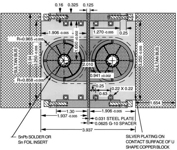
Figure 2-3 shows a cross-sectional view of a joint design for the ITER magnet which connects the ends of a cable to the power supply. The end of a cable is stripped of it's outer metal jacket and the strands within are straightened out, and soldered together. It is then wrapped with a metal sheath and soldered to the current bus line. This configuration, where the contact between the current bus and the end of the cable is long, ensures that the current distribution flowing to the cable is more or less uniform. We can model this joint interface in three parts. Figure 2-4 shows the three regions. The leftmost region (2) models the metal-to-metal contact between the bus and the joint. Region 1 is the joint itself where we will assume that the diffusion time of the currents are negligible thus capturing the uniform current behavior of a real joint.
The governing equation is
V x V x E = -o (2.51)
In the joint region (1), the conductivities are anisotropic. The same set of equations that are used to solve the cable region are also needed for the joint region. The difference is that aL here is homogenous since the solder that fills the void between strands makes a uniform conductivity close to the conductivity of copper. Therefore,
0"1= -cu.
In region 2, the conductivity is simply that of copper -homogeneous and isotropic.
The differential equation is
V2E = 0o ta
R
(2.52)2.5. FORMULATION OF BOUNDARY CONDITIONS
J-J:
UPPER JOINT
0.16 0.325 0.125 j'4O1.30 - 1.906 -0.005 No 1.937 -o.oo005s S-0-0.031
STEEL PLATE ~'1- 0.0625 G-10 SPACERSn FOIL INSERT CONTACT SURFACE OF U
SHAPE COPPER BLOCK
TITLE: US PREPROTOTYPE JOINT SAMPLE IVER.: 4.50 IDATE: 19950316 ICYGI P. u21
UNITS: INCHES ITOLERANCE: UNLESS OTHERWISE SPECIFIED, .XX±.01,. XXXi.005 ISCALE: 1
joint (1)
metal contact (2) cable
I I
-I 0
Figure 2-4: Model of joint at source.
the boundary conditions are at z -1,
E(2) = Scu7 7 R 2 Er 2)= 0 E( 2) = 0 at z = 0, E ( 1 )- E 2)
E(1)
= E(2)
aloE 1 ) = aOcuE!2 )E
1
)
=
E
•
2)
=
o0
at r = R, (2.54)(2.55)
The superscripts (1) and (2) indicate the regions.
2.5. FORMULATION OF BOUNDARY CONDITIONS
Region (2)
If we were to assume small enough changes in B such that V x E = - ° B 0
coupled with a divergence-free current density which yields V - J = V -E = 0, these
two conditions imply that the scalar potential can be used.
S= -V(I (2.56)
(I in turn would satisfy Laplace's equation.
V24( = 0
(2.57)
To be consistent with the boundary conditions at r = R and z = -1, the general
solution for (P should be
I sin m
1
(D(2) (r, , z)= - Z +mnJm(knr)
cosh k,(z + 1) (2.58) cR n m cosm
J
Therefore Or = n m Jm(k - sin m cosh k,z (2.59) k Ik cos mO 1 4m { sin m } E0 = - Jm(knr) cosh knz (2.60) Er o n m r1-
cosmO &I
sin m
1
Ez = = a R2 +•• knJm(knr) ssmO sinh knz (2.61) Oz crirR n m cos mOk, has to satisfy the condition that
mJm(kR) - knrJm-l(kR) = 0 (2.62)
Region (1)
The last equation of (2.54) dictates the continuity of current. The summation term
in E,2 ) is scaled by both acu/all and sinh k,l. Therefore, neglecting the c terms and
assuming I << 1/k,, we obtain
E(1) = acuE(2)
I (2.63)
all-R 2
We have arrived at a simple and straightforward boundary condition at z = 0. The
joint will just be an extension of the cable with a different perpendicular conductivity and can be solved numerically. The boundary condition at the end of the joint, at the joint-metal contact interface, will be that of a uniform field distribution, it's magnitude determined by the current source. The fields and thereby the loss in the metal contact region can be found by equating the transverse fields at the boundary
z = 0 to find the coefficients E(2) and E(2)
As mentioned before, the above derivation is only for one joint design. The
con-dition on dipole fields and therefore currents at z = 0 is identical to that of an
open-ended cable. There is a range of conditions on the ends, each dictated by the type of joint design.
For the US-DPS coil, ribbon joints were built. These are manufactured by taking strands at the end of the cable, straightening them out and flattening the cable geometry from a circular to a flat rectangular cross-section. The strands are then
2.5. FORMULATION OF BOUNDARY CONDITIONS
soldered together and placed in a metal sheath. Because the strands were soldered together such that there is no void space, the transverse contact resistivity approaches that of the solder metal resistivity and is much higher than the rest of the cable. However, a, is still much smaller than all. This becomes a true multi-regional and anisotropic problem.
It has been proposed, but not implemented, that the strands are stripped of their normal metal and compacted together. This would represent the opposite extreme to
the ITER joint. Now, ai = all and the boundary condition at z = 0 becomes Er = 0
or 4 = 0. This is equivalent to the short-circuited end condition.
2.5.2
Magnet in persistent mode
In applications where magnets are not connected to any external source, the magnet is said to be operating in persistent mode. It is one of the great advantages of having
superconducting cables - the decay time is so large that any flux or current trapped
in the magnet will stay trapped for a long time. This mode of operation can be found in NMR machines and can be used for such applications as MAGLEV where the cost of having an onboard power supply for each electromagnetic magnet is impractical.
Boundary Conditions
The major difference between this problem and that of a magnet with a current source is that here, the transport current is no longer a source term. In fact, the current is an unknown variable, a combination of an applied and an induced current. Unlike the previous case where any induced back EMF is absorbed by the power supply (i.e. any induced voltage appears across the source), the induced current produced by the
Figure 2-5: Sketch of magnet in an electrically closed loop.
EMF can determine a significant portion of the total transport current. Thus,
I = IA + Iind
(2.64)
Consider one single loop of radius Ro as shown in figure 2-5. The specifications for boundary conditions are a bit tricky due to the implicit curvature of the problem.
However, one can show that if all terms of order R/Ro or higher are neglected, the formulation for a straight wire case can be used here. This is saying that the size of
the magnet is so large compared to the radius of the cable, the curvature effect can be neglected.
Faraday's law dictates that for a time-varying magnetic field, the electric field along the cable must satisfy
Ed-= ata
c B
(2.65) where A is the total flux linked.
The flux linkage term consists of an external field, field due to current in the
-4-2.5. FORMULATION OF BOUNDARY CONDITIONS
cable, and any multipole fields. Since multipole fields die away as rn and since the
magnitude of these fields are already small, the contribution to the flux linkage due to these induced terms will be neglected.
The externally applied magnetic field is uniform. The induced field is a function of the transport current.
J-?~
Ezdz = -BA rR2 _ -9#
Bind(I,
r, €, z)da (2.66)This can be rewritten as
r (rRo d A
J
(Ez + O Az)dz = -AirR27r- o t
0 (2.67)
where Az corresponds to the vector potential of the loop This saves us some time in calculating the field due to a having to integrate it over the internal area of the loop. for Az(r, €) can be found in Jackson's book[12]. However effect of the curvature of the loop, A, is dependent only on r = R,
AZ = ol C
27r
current at the boundary. loop of current and then The complete expression since we are ignoring the
I. At the cable boundary
(2.68) where C is a constant calculated from the average value of Az around the cable
perimeter and is dependent on the size of the cable. As an example, for R = 1.9cm
and Ro = 19cm, C P 4.9.
Therefore, we have an additional boundary condition that links the current to the applied magnetic field.
c(E (r= R) + LoIC) dz = -A Ro
joint-joint -metal contact
joint cable'
Figure 2-6: Model of persistent switch (joint that closes the loop).
End conditions
Since the ends are wrapped on itself, the term "end" conditions is a bit misleading but we will use this terminology since the specifications are fairly similar to that of a magnet connected to a source. More commonly, this joint interface is referred to as
a "persistent switch".
Figure 2-6 shows the model of the joint between the two ends of the coil. Again, we assume that the current is uniform in the metal contact region. Here is the boundary
condition at z = 1 and 27rRo - 1.
I
Ez (2.70)
This also means that there is a resistive voltage drop across the metal region. Since
This also means that there is a resistive voltage drop across the metal region. Since
LUIEV
I I0 1
2nRo -I 0 1
2.6. CONCLUSION
we know that the current is uniform, the voltage is simply
Vres = - I (2.71)
The boundary condition is now refined to
(Ez
+
27C)dz -
acurR 2I
=
-A
2o
(2.72)
2.6
Conclusion
An elegant yet powerful electromagnetic model has been developed for the study of current distribution and AC loss in composite superconductors. An ordering system, which captures most of the physics of the problem, has been instrumental in reducing
the governing equations to a tractable form. Two equations for two unknowns, Ell
(the electric field along the direction of a superconducting filament or strand) and 1(the transverse potential), describe the entire system.
To complete the formulation of the model, a general set of boundary conditions were derived for circulary shaped cables with joints at both ends. These cable ends can be connected to a source or with each other in "persistent mode".
Chapter 3
Analytic Results of Limiting Cases
The objective of this chapter is to derive several analytic solutions from the governing equations in special limits. It is always desirable to be able to rely on closed-form solutions for any problem if they are available. Numerics are useful when analytic results cannot be obtained. Some simple geometries have analytic solutions thereby allowing certain physical laws describing the behavior of these strands and cables to be ascertained.
This chapter outlines the derivations to the solutions of untwisted or single twist pitch composite conductors with various end conditions. The conductivity all will be treated as a constant. Results of interesting limits to these solutions will be analyzed
and, when possible, compared to existing literature.
3.1
Open-circuited straight cable
The first limiting case is that of a straight, finite section of cable of length 2L which is open-circuited at both ends. The wires inside are untwisted and no saturation occurs.
________________iI[
p
I z
-L L
Figure 3-1: Untwisted finite length cable.
Since there is no twisting, p = 0 and p4 = 0 so that 6ii = 6,z. The differential
equations are reduced to simply
V I(Ell + ) = I-o allEll (3.1)
u
1
V4
=
,l
El
(3.2)
Taking - of (3.2) and substituting into (3.1) yields one equation for Ell. For
simplicity, we assume = 0, i.e. we are solving for stationary solutions.
SVT
+ 2 El i
+o
ao
0 llEll
0- (3.3)(a
a
a2)
at
These solutions can be applied with a decent amount of accuracy for slow field variations. For sinusoidal field variations, the time derivative does not complicate the analysis. For this example, we will examine a ramped field to illustrate how the losses scale. In addition, no saturation of the wires and uniform conductivities are also assumed.
The boundary conditions are
I 1 1 1 1 1 1 1


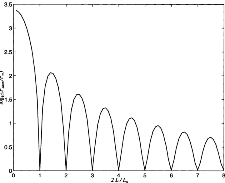
![Figure 3-7: Power loss for open ends normalized to infinite cable as compared to analytically-derived expression from [13].](https://thumb-eu.123doks.com/thumbv2/123doknet/14426618.514337/82.918.88.808.237.818/figure-power-normalized-infinite-compared-analytically-derived-expression.webp)