HAL Id: hal-01607479
https://hal.inria.fr/hal-01607479
Submitted on 2 Oct 2017
HAL is a multi-disciplinary open access
archive for the deposit and dissemination of
sci-entific research documents, whether they are
pub-lished or not. The documents may come from
teaching and research institutions in France or
abroad, or from public or private research centers.
L’archive ouverte pluridisciplinaire HAL, est
destinée au dépôt et à la diffusion de documents
scientifiques de niveau recherche, publiés ou non,
émanant des établissements d’enseignement et de
recherche français ou étrangers, des laboratoires
publics ou privés.
Avoiding Intermediate Files
Théophile Terraz, Alejandro Ribes, Yvan Fournier, Bertrand Iooss, Bruno
Raffin
To cite this version:
Théophile Terraz, Alejandro Ribes, Yvan Fournier, Bertrand Iooss, Bruno Raffin. Melissa: Large Scale
In Transit Sensitivity Analysis Avoiding Intermediate Files. The International Conference for High
Performance Computing, Networking, Storage and Analysis (Supercomputing), Nov 2017, Denver,
United States. pp.1 - 14. �hal-01607479�
Melissa: Large Scale In Transit Sensitivity Analysis Avoiding
Intermediate Files
Théophile Terraz
Univ. Grenoble Alpes, Inria, CNRS, Grenoble INP, LIG
38000, Grenoble, France [email protected]
Alejandro Ribes
EDF Lab Paris-Saclay France [email protected]
Yvan Fournier
EDF Lab Paris-Chatou France [email protected]
Bertrand Iooss
EDF Lab Paris-Chatou France [email protected]
Bruno Ra�n
Univ. Grenoble Alpes, Inria, CNRS, Grenoble INP, LIG
38000, Grenoble, France bruno.ra�[email protected]
ABSTRACT
Global sensitivity analysis is an important step for analyzing and validating numerical simulations. One classical approach consists in computing statistics on the outputs from well-chosen multiple simulation runs. Simulation results are stored to disk and statis-tics are computed postmortem. Even if supercomputers enable to run large studies, scientists are constrained to run low resolution simulations with a limited number of probes to keep the amount of intermediate storage manageable. In this paper we propose a �le avoiding, adaptive, fault tolerant and elastic framework that enables high resolution global sensitivity analysis at large scale. Our approach combines iterative statistics and in transit process-ing to compute Sobol’ indices without any intermediate storage. Statistics are updated on-the-�y as soon as the in transit parallel server receives results from one of the running simulations. For one experiment, we computed the Sobol’ indices on 10M hexahedra and 100 timesteps, running 8000 parallel simulations executed in 1h27 on up to 28672 cores, avoiding 48TB of �le storage.
KEYWORDS
Sensitivity Analysis, Multi-Run Simulations, Ensemble Simulation, Sobol’ Index, In Transit Processing
ACM Reference format:
Théophile Terraz, Alejandro Ribes, Yvan Fournier, Bertrand Iooss, and Bruno Ra�n. . Melissa: Large Scale In Transit Sensitivity Analysis Avoiding Intermediate Files. In Proceedings of Super Computing conference, Denver, Colorado USA, November 2017 (SC’17),14pages.
DOI:
1 INTRODUCTION
Computer simulation is undoubtedly a fundamental question in modern engineering. Whatever the purpose of a study, computer models help the analysts to forecast the behavior of the system under investigation in conditions that cannot be reproduced in physical experiments (e.g. accidental scenarios), or when physical experiments are theoretically possible but at a very high cost. To
SC’17, Denver, Colorado USA . .
DOI:
improve and have a better hold on these tools, it is crucial to be able to analyze them under the scopes of sensitivity and uncertainty analysis. In particular, global sensitivity analysis aims at identifying the most in�uential parameters for a given output of the computer model and at evaluating the e�ect of uncertainty in each uncertain input variable on model output [22,41]. Based on a probabilistic framework, it consists in evaluating the computer model on a large size statistical sample of model inputs, then analyzing all the results (the model outputs) with speci�c statistical tools.
Sensitivity analysis for large scale numerical systems that simu-late complex spatial and temporal evolutions [10,33,42] remains very challenging. Such studies can be rather complicated with numerical models computing the evolution in time with tens of variables on thousands or millions of grid points, systems cou-pling several models, prediction systems using not only one model but also observations through, for instance, data assimilation tech-niques.
Multiple simulation runs (sometimes several thousand) are re-quired to compute sound statistics for global sensitivity analysis. Current practice consists in running all the necessary instances with di�erent set of input parameters, store the results to disk, often called ensemble data, to later read them back from disk to compute the required statistics. The amount of storage needed may quickly become overwhelming, with the associated long read time that makes statistic computing time consuming. To avoid this pitfall, scientists reduce their study size by running low resolution sim-ulations or down-sampling output data in space and time. Today terascale and tomorrow exascale machines o�er compute capabili-ties that would enable large scale sensitivity studies. But they are unfortunately not feasible due to this storage issue.
Novel approaches are required. In situ and in transit processing emerged as a solution to perform data analysis starting as soon as the results are available in the memory of the simulation. The goal is to reduce the data to store to disk and to avoid the time penalty to write and then read back the raw data set as required by the classical postmortem analysis approach. But to our knowledge no solution has been developed to drastically reduce the storage needs for sensitivity analysis.
In this paper, we focus on variance-based sensitivity indices, called Sobol’ indices, an important statistic value for sensitivity
analysis. We propose a new approach to compute Sobol’ indices at large scale by avoiding to store the intermediate results produced by the multiple parallel simulation runs. The key enabler is a new iterative formulation of Sobol’ indices. It enables to update Sobol’ indices on-the-�y each time new simulation results are available. To manage the simulation runs as well as the in transit computation of iterative statistics, we developed a full framework, called Melissa, built around a fault tolerant parallel client/server architecture. The parallel server is in charge of updating the Sobol’ indices. Parallel simulations, actually groups of simulation as detailed in this paper, run independently. Once a simulation starts, it connects to the server and forwards the output data available at each timestep (or at a su�ciently resolved sampling in time) for updating statistics. These data can then be discarded. The bene�ts of our approach are multiple:
• Storage saving: zero intermediate �les and a memory requirement on the server side in the order of the outputs of one simulation run.
• Time saving: simulations run faster when sending data to the server than when writing their results to disk, and our one-pass algorithm does not need to read back some huge amount of data from disk to compute the Sobol’ indices. • Ubiquitous: performance and scalability gains enable to
compute ubiquitous multidimensional and time varying Sobol’ indices, i.e. everywhere in space and time, instead of providing statistics for a limited sample of probes as usually done.
• Adaptive: simulation groups can be de�ned, started or interrupted on-line according to past runs behavior or the statistics already computed.
• Fault tolerance: only some lightweight bookkeeping and a few heartbeats are required to detect issues and restart the server or the simulations, with limited intermediate result loss.
• Elasticity: simulation groups are independent and con-nect dynamically to the parallel server when they start. They are submitted as independent jobs to the batch sched-uler. Thus, the scheduler can adapt the resources allocated to the application during the execution.
The experiment we run for this paper is based on a parallel �uid simulation ensemble on a 10M cells mesh and 100 timesteps. We run 8000 simulations that generate a total of 48TB of data that are assimilated on-the-�y and thus do not need to be stored on disk. Simulation outputs are not down-sampled. Melissa computes �rst order and total Sobol’ indices on all timesteps and mesh cells. The full sensitivity analysis runs in about 1h27 using up to 28672 cores simultaneously, with 2.1% of the CPU time used by the server.
The paper is organized as follows. After an overview on sensitiv-ity analysis (Sec.2), iterative Sobol’ indices are introduced (Sec.3). Melissa architecture is detailed (Sec.4), followed by experimental re-sults (Sec.5). Related works are discussed (Sec.6) before concluding remarks (Sec.7).
2 SENSITIVITY ANALYSIS: AN OVERVIEW
Sensitivity studies are an important application of uncertainty quan-ti�cation in numerical simulation [42]. The objective of such studies
f Y
X1
X2
...
Xp
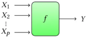
Figure 1: A simple solver f taking p input parameters X1to
Xp, and computing a scalar output Y.
can be broadly viewed as quantifying the relative contributions of individual input parameters to a simulation model, and determining how variations in parameters a�ect the outcomes of the simulations. These input parameters include engineering or operating variables, variables that describe �eld conditions, and variables that include unknown or partially known model parameters. In this context, multi-run studies treat simulations as black boxes that produce outputs when a set of parameters is �xed (Fig.1).
2.1 Introduction to Sobol’ Indices
Global sensitivity analysis is an ensemble of techniques that deal with a probabilistic representation of the input parameters [41] to consider their overall variation range. Variance-based sensitiv-ity measures, also called Sobol’ indices [43], are popular among methods for global sensitivity analysis [22]. They decompose the variance of the output, Y, of the simulation into fractions, which can be attributed to random input parameters or sets of random inputs. For example, with only two input parameters X1and X2
and one output Y (Fig.1), Sobol’ indices might show that 60% of the output variance is caused by the variance in the �rst parameter, 30% by the variance in the second, and 10% due to interactions between both. These percentages are directly interpreted as measures of sensitivity. If we consider p input parameters, the Sobol’ indices can identify parameters that do not in�uence or in�uence very slightly the output, leading to model reduction or simpli�cation. Sobol’ indices can also deal with nonlinear responses, and as such they can measure the e�ect of interactions in non-additive systems. Mathematically, the �rst and second order Sobol’ indices [43] are de�ned by:
Si =Var(E[Y |Xi])
Var(Y ) , Sij=Var(E[Y |XiXj])
Var(Y ) Si Sj, (1)
where X1, . . . ,Xpare p independent random variables. In Eq. (1), Si
represents the �rst order sensitivity index of Xiwhile Sijrepresents
the e�ect of the interaction between Xiand Xj. Higher-order
inter-action indices (Sijk, . . . ,S1...p) can be similarly de�ned. The total
Sobol’ indices express the overall sensitivity of an input variable Xi: STi =Si+ X j,i Sij+ X j,i,k,i, j <k Sijk+ . . . +S1...p (2)
2.2 Ubiquitous Sensitivity Analysis
Based on simple statistical measures (variance, distribution func-tion, entropy, ...), the algorithms of global sensitivity analysis have mainly been developed for a scalar output [22]. This case is illus-trated in (Fig.1) and corresponds to:
... Simulation Results 1 Simulation Results 2 x1 x2 x3 x4 x5 t1t2t3t4t5 x1 x2 x3 x4 x5 t1t2t3t4t5 x1 x2 x3 x4 x5 t1t2t3t4t5 x1 x2 x3 x4 x5 t1t2t3t4t5 Simulation
Results N UbiquitousAnalysis
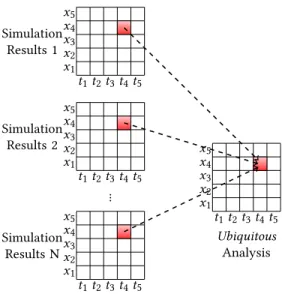
Figure 2: Ubiquitous spatio-temporal sensitivity analysis. Statistics are computed from N simulation runs for all spa-tial variables x1, ...x5and all timesteps t1, ...,t5.
where f (.) is the numerical model under study. However, numerical simulation results are often multidimensional �elds varying over time, which cannot be represented by a single scalar value. In this general case, the model becomes:
Y (x, t ) = f (x, t, X1, . . . ,Xp), (4)
where x represents all the cells (or points) in a 2D or 3D mesh and trepresents the discrete time of the simulation (an index over the timesteps). In this article we deal with complex functional outputs Y (x, t ), which cannot be analysed by use of scalar Sobol’ indices as de�ned in Eq. (1). Thus, we call ubiquitous Sobol’ indices the generalisation of Sobol’ indices for outputs Y (x, t) representing multidimensional �elds varying over time. Ubiquitous Sobol’ in-dices are also multidimensional and time varying (Si(x, t )) (Fig.2).
Existing works have revealed strong computational di�culties for the sensitivity estimation step, mainly caused by the storage bottleneck. For this reason, the analysis of [32] is restricted to a small number of timesteps. Indeed, computing sensitivity indices with the classical techniques requires the storage of all the simula-tion outputs (several thousands of �nely-discretized spatial maps in [32]). To our knowledge, no literature exists to solve this problem, and the present paper is the �rst work dealing with this issue for a global sensitivity study. We propose to avoid storing the simulation outputs by performing computations in transit.
3 IN TRANSIT SENSITIVITY ANALYSIS
3.1 Iterative Statistics
Computing statistics from N samples classically requires O(N ) memory space to store these samples. But if the statistics can be computed iteratively, i.e. if the current value can be updated as soon as a new sample is available, the memory requirement goes down to O(1) space. This type of iterative formula is also called one-pass, online or even parallel statistics. Sobol’ indices require the mean,
variance and covariance, that have known iterative formulas as found in [34].
With this approach, not only simulation results do not need to be saved, but they can be consumed in any order, loosening synchronization constraints on the simulation executions (Fig.2).
3.2 Sobol’ Indices
Our goal is to compute in transit the Sobol’ indices of each input parameter Xi (Fig.1). Before de�ning iterative Sobol’ indices
for-mulas, we discuss the classical ways of estimating Sobol’ indices in a non-iterative fashion. It consists in estimating the variances of conditional expectation (Eq. (1)). We explain below the so-called pick-freeze scheme that uses two random independent and identi-cally distributed samples of the model inputs [21,24,43].
We �rst de�ne the p variable input parameters of our study as a random vector, with a given probabilistic law for each parameter. We then randomly draw two times n sets of p parameters, to obtain two matrices A and B of size n ⇥ p. Each row is a set of parameters for one simulation.
A =*... , a1,1 · · · a1,p .. . . .. an,1 an,p +/ // -; B =*... , b1,1 · · · b1,p .. . . .. bn,1 bn,p +/ // -For each k 2 [1,p] we de�ne the matrix Ck, which is equal to
the matrix A but with its column k replaced by column k of B. Each row of each matrix is a set of input parameters:
Ck= *. .. .. .. .. , a1,1 · · · a1,k 1 b1,k a1,k+1 · · · a1,p .. . ... ... ... ... ai,1 · · · ai,k 1 bi,k an,k+1 · · · ai,p
.. . ... ... ... ... an,1 · · · an,k 1 bn,k an,k+1 · · · an,p +/ // // // // -Then, a study consists in running the n ⇥ (p +2) simulations de�ned by the matrices A, B and Ckfor k 2 [1,p].
For each matrix M with n rows, 8i 2 [1,n], let Mibe the ithrow
of M, and M[:i]the matrix of size i ⇥ p built from the i �rst lines of
M. For example :
Cki =⇣ai,1 · · · ai,k 1 bi,k ai,k+1 · · · ai,p⌘
and C[:i]k =*... , a1,1 · · · a1,k 1 b1,k a1,k+1 · · · a1,p .. . ... ... ... ... ai,1 · · · ai,k 1 bi,k an,k+1 · · · ai,p
+/ // -Let YA
i be the result of f (Ai), and YA2 Rnthe vector built from
component i of YA
i , 8i 2 [1,n]. We de�ne YiBand YBin the same
way, as well as YCk
i and YC
k
8k 2 [1,p].
Let V(x) be the unbiased variance estimator, and Co (x, ) the unbiased covariance estimator, as de�ned in [34]. First order Sobol’ indices Skcan be estimated by the following formula, called Mar-tinez estimator [4]: Sk( f , A, B) = Co (YB,YC k ) p V(YB) q V(YCk) , (5)
while total order Sobol’ indices STkare estimated by: STk( f , A, B) =1 Co (YA,YC k ) p V(YA) q V(YCk) (6)
There are many others estimators (see for example [38]) relying on the matrices A, B and Ckto compute the variance and the
co-variance with di�erent formulas. We use the Martinez estimator because it provides a very simply-expressed asymptotic con�dence interval [4] (see Section3.4), easy to compute in an iterative fashion. In addition, it has been shown to be unbiased and one of the most numerically stable estimator [4].
Notice that all the couples of rows in the matrix pair (A, B) are independent of each other. If needed, for instance convergence not achieved (Sec.3.4), it is statistically valid to generate randomly new couples of rows.
3.3 Iterative Sobol’ Indices
Each estimator of the Sobol’ indices corresponds to a speci�c co-variance formula. As the iterative statistics formulas are exact with respect to the non-iterative ones, we focus here on the Martinez estimation method, because it is simply expressed (with variance and covariance terms) and provides a con�dence interval in the non-iterative case. One of Martinez method main advantage is that its associated con�dence interval is easily computable in the iterative case.
Since variances and covariances can be updated iteratively [34,
44], partial Sobol’ indices Ski+1can be computed from Y[:i]A , Y[:i]B
and YCk
[:i]with the same formula (Eq.5):
Ski( f , A[:i],B[:i]) =
Co (Y[:i]B ,Y[:i]Ck) q
V(Y[:i]B )qV(Y[:i]Ck)
(7)
To update the kth�rst order Sobol’ index, access to YB
i+1and YC
k
i+1
is required. As each index update needs two data and each data is required for at least two indices, we need to know YA
i+1, Yi+1B and
Yi+1Ck to update all the indices. These data correspond to the p + 2 simulation results coming from the ithrow of each matrix. We
gather these p + 2 simulations into one simulation group (executed synchronously as we will see in section4). All the n simulation groups remain independent and can be computed asynchronously.
3.4 Convergence Control
Martinez formula provides an asymptotic con�dence interval for the Sobol’ indices [4]. Theoretically, it is valid under a Gaussian distribution of the simulation outputs. We experimented that in practice it gives a good overview of the index accuracy.
The classical 95% con�dence level at iteration i is given by:
Prob (Sk2 [tanh(12log(1 + S1 Ski ki
) p1.96 i 3), tanh(12log(1 + Ski
1 Ski) +p1.96i 3)]) ' 0.95 (8)
Prob (STk2 [1 tanh(12log(2 STki
STki ) + 1.96 p i 3), 1 tanh(12log(2 STki STki ) p1.96 i 3)]) ' 0.95 (9) These formulas can be computed at each update of Sobol’ indices. They only require the size i of the sample and the current value of the Sobol’ index estimate (see Section3.3).
To avoid unnecessary computations, one can check the con-vergence of the Sobol’ indices. Once these indices reach a given con�dence interval, the remaining pending simulation jobs can be cancelled. On the contrary, if the con�dence interval at the end of the study is not satisfactory, the system could continue to iterate by submitting new simulations.
4 SOFTWARE FRAMEWORK
Launcher
Parallel Server
Batch Scheduler Pending jobs: groups k, l, ...
Group i
Group j
Figure 3: Melissa deployment overview. The launcher runs on the front node and interacts with the batch scheduler for submitting job and querying their status. Simulation groups are started when resources are available on the machine (groups i and j are running while groups k and l are waiting to be scheduled). Each one connects to Melissa Server (par-allel) and funnels its outputs as soon as available. Melissa Server regularly sends reports to the launcher for detecting failures or adapting the study (stop/start simulations).
4.1 Melissa Architecture
Melissa (Modular External Library for In Situ Statistical Analysis) is an open source framework1that relies on a three tier architecture
(Fig.3). The Melissa Server aggregates the simulation results and updates iterative statistics as soon as a new result is available. The Melissa clients are the simulation groups providing outputs to the server. Melissa Launcher is a script running on the front node in charge of creating, launching, and supervising the server and clients.
As mentioned in the previous section, p + 2 simulations are run synchronously in a group (p being the number of variable input parameters) to keep low memory requirements on the server side. These simulations need to provide the results for the same timestep to the server so the server can update all Sobol’ indices and discard the data.
Notice that beside Sobol’ indices, Melissa can be con�gured to compute other iterative statistics on the same data but only on YAand YB(input parameters are not independent for the other simulations from a group). For instance [34] proposes iterative formulas for higher order moments (skewness, kurtosis and more), which could be useful for uncertainty propagation studies.
4.1.1 Melissa Server.The server is parallelized with MPI and runs on several nodes. Increase in the number of nodes is �rst motivated by a need for more memory. The amount of memory needed is in the order of the size of the results of one simulation for each computed statistic (number of timesteps ⇥ the number of cells or points in the mesh ⇥ the number of statistics computed), plus the number of messages in the inboud queue (user de�ned). Memory size could also be extended by using out-of-core memory (such as burst bu�ers for instance). The simulation domain is evenly partitioned in space among the di�erent processes at starting time. Updating the statistics is a local operation that requires neither communication nor synchronization between the server processes. The server processes continuously check for incoming messages to update their local statistics. The data sent by the clients can be processed in any order.
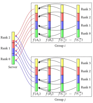
Rank 0 Rank 1 Rank 2 Rank 3 f (Bi) f (C1i) ... f (Cni) f (Ai) Group i Rank 0 Rank 1 Rank 2 Rank 3 f (Bj) f (C1j) ... f (Cnj) f (Aj) Group j Rank 0 Rank 1 Rank 2 Server
Figure 4: Two simulation groups i and j, each running n + 2 parallel simulations (4 processes), are connected to the Melissa parallel server (3 processes). Each time the results of a new timestep are available within a group, the data are �rst gathered on the main simulation processes (black ar-rows), before to be redistributed to the server (blue and red arrows).
4.1.2 Two Stages Data Transfers.To limit the number of mes-sages sent to Melissa Server, data from simulation groups are trans-ferred in two stages (Fig.4). For a given simulation group, the data from the ranks i of the p + 2 simulations are gathered on the rank i of a designated main simulation (black arrows). Next, each process from this main simulation redistributes the gathered data to the necessary destination processes of the Melissa Server (red and blue arrows).
The p + 2 simulations inside a group are MPI programs started together in a MPMD mode that enables getting a global commu-nicator amongst all simulation processes. Gathering the data to the main simulation is simply performed through a MPI_Gather collective communication.
4.1.3 Dynamic Connection to Melissa Server.When a group starts, the main simulation dynamically connects to Melissa Server. Each main simulation process opens individual communication channels to each necessary server process. First, process zero from the main simulation connects to the server main process to retrieve information related to data partitioning and process addresses on the server side. The information is sent to the other main simulation processes that next open direct connections to the necessary target server processes. Every time new results are gathered on the main simulation, its processes push the results toward Melissa Server.
Melissa was designed to keep intrusion into the simulation code minimal. Melissa provides 3 functions to integrate in the simula-tion code through a dynamic library. The �rst funcsimula-tion (Initialise) allocates internal structures and initiates the connection with the server. At each timestep, the second function (Process) �rst gathers the data within the simulation group before to send them to Melissa Server. The third function (Finalize) disconnects the simulation and releases the allocated structures.
For the client/server support, we use the Z���MQ communica-tion library [20], a well known and reliable communication library for distributed applications. Z���MQ is a multi-threaded library that takes care of the asynchronous transfer of messages between a client and a server. Messages are bu�ered on the client and server side if necessary, to regulate data transfers and reduce the need for blocking either the server or the client. Bu�er sizes can be user controlled. Thus message transfers are performed asynchronously in the background by Z���MQ threads on the main simulation side as well as on Melissa Server side. Communications only become blocking when both bu�ers are full.
Z���MQ proved easy to use in an HPC context. Its main lim-itation is the lack of direct support for high performance net-works like In�niband or Omni-Path. Z���MQ relies on sockets and the TCP transport protocol, not enabling to take full bene-�t of the capabilities of the underlying network. We envision to move to RDMA based dynamic connections in the future (using MPI_Comm_connect for instance).
So far the N ⇥ M data redistribution pattern between a simula-tion group and the Melissa Server is static. Moving to a dynamic redistribution scheme would enable to support simulations per-forming dynamic data partitioning. Supporting simulations that use di�erent meshes (adaptive mesh re�nement for instance), would require to interpolate the data to a common mesh resolution at each timestep to properly update Sobol’ indices.
4.1.4 Melissa Launcher.Melissa Launcher is in charge of gener-ating the parameter sets and the study environment. After cregener-ating the con�guration �les, it submits a �rst job to the batch scheduler to start Melissa Server. Once this job is running, the launcher re-trieves the server address that it provides, and launch the simulation groups. Each simulation group is submitted independently to the batch scheduler. They can be submitted all at once or at a more regulated pace if there is a risk to overload the batch scheduler. For instance we were limited to 500 simultaneous submissions for running our experiments. The launcher also plays a key role for fault tolerance support as detailed in next section.
For each new use case, the user needs to provide a script for the Melissa Launcher to generate the parameter sets and to launch the simulation groups.
4.1.5 Convergence Control.In the current implementation, Melissa Server computes the con�dence intervals (Sec.3.3) for all computed Sobol’ indices each time they are updated. It can either output a map of con�dence interval values, or only keep the largest value over all the mesh and all the timesteps.
We could further take advantage of con�dence intervals to im-plement a loopback control. Once the launcher detects that the con�dence intervals are bellow a given threshold, it could request the launcher to kill the running simulation groups and stop the ap-plication. Conversely, if the convergence criteria is not reached new matrix rows could be generated on-the-�y (by randomly drawing new rows for A and B) to run new simulation groups.
4.2 Fault Tolerance
Melissa asynchronous client/server architecture and the iterative statistics computation enable to support a simple yet robust fault tolerance mechanism. We support detection and recovery from failures (including straggler issues) of Melissa Server and simulation groups. We consider a simulation group as a single entity. If a sub-component fails (one simulation for instance) the full group is considered failed. Finer grain fault tolerance would require some checkpointing/restart capabilities in the simulation that we do not assume to be available.
4.2.1 Accounting.Each Melissa Server process keeps the list of �nished and running simulation groups with its id and the timestep of the last message received from this group. These data together with the current statistics values are periodically checkpointed to �le.
Melissa Server processes systematically apply a discard on replay policy to all received messages. If the received message has a timestep id lower than the last one recorded for this simulation group it is discarded. The goal is to prevent integrating multiple times in the statistics the same timestep from the same group id, which could occur when a simulation group is restarted. As we will see, this policy enables to recover from various failure situations.
However, merging results from di�erent instances of the same simulation may not always be considered safe, for instance when executions are not numerically stable enough due to non determin-ism. In this case, it is delicate to implement a reasonable rollback recovery process to undo only the statistic updates from a given
simulation: at any point in time the cumulated statistics can inte-grate results from several running simulations. One alternative is to disable the discard on replay policy. A failing simulation group is never restarted. Instead, a new one is generated and run. It is statistically valid to replace the failing group by another group running with a new randomly generated couple of rows (for A and B).
4.2.2 Simulation Group Fault.We assume that a group com-putes and sends its timesteps in increasing order, as it is the case for most simulation codes (and messages stay in that order on the reception side). A server process considers a group started if it re-ceived at least one message, �nished if it rere-ceived the �nal timestep id.
Melissa Server performs regular checkpoints where each process saves the current computed statistics with the list of simulation states.
We distinguish two cases of simulation group failure that need di�erent detection strategies:
• At least one server process received at least one message from this simulation group (un�nished group).
• No server process received any message from this simula-tion group (zombie group).
For detection of un�nished groups, we de�ne a timeout between two consecutive messages received from a given simulation group. Each time a server process receives a message from a group, it records its reception time. Each server process periodically checks for each running group that message waiting time did not exceed the timeout. If a timeout is detected, the process noti�es the Melissa Launcher. The launcher kills the corresponding job if it is still running, and restarts a new instance of this simulation group.
The second case (zombie group) occurs if Melissa Launcher sees a group as running through the batch scheduler, but that group never actually sent any message to Melissa Server for a long time. Periodically, processes from Melissa Server send the list of running and �nished jobs to Melissa Launcher. Upon reception of this list, Melissa Launcher checks that jobs it sees as running or �nished have at least sent one message to at least one server process before a given timeout measured since the simulation started. The job run time is retrieved from the batch scheduler. If no message was received, the job is considered as failing. The launcher kills it and restarts a new instance. In the meantime if the server received some messages from this instance, they will be used to update statistics, but the duplicate messages that will produce the new instance will be discarded (discard on replay policy). This protocol also covers the cases where a job is considered �nished by the launcher while the server has never received any message.
Notice that Z���MQ has its own internal fault detection and recovery process, in case of disconnection for instance. If it fails to recover or takes too long, Melissa will consider the job as failing and trigger the kill and restart process.
The fault tolerance protocol exposed above is also e�ective when the batch scheduler discards or kills the job of a simulation group (reservation walltime exceeded for instance).
The Melissa Launcher also counts the number of retries for each simulation group. If it reaches a given threshold, the launcher gives up this simulation group. The failure can come from a non
valid combination of input parameters. Drawing a new set of input parameters to replace the failing group is always possible but it would introduce a bias in the statistics. This is thus not Melissa default behavior.
In all cases, the user gets a clear vision of the actual data that were accumulated to compute the results through the detailed report of failures and restarts the Melissa Server provides.
4.2.3 Melissa Server Fault.Melissa Launcher implements a time-out based heartbeat with the server processes, as well as regular jobs status checkups. If it considers the server as failing, the launcher kills it, killing as well all pending and running simulation groups. Next, it launch a new server instance that restarts from the last avail-able checkpoint �le. Upon restart, the server noti�es the launcher about its list of �nished and running groups at the time of the backup. Eventually the launcher restarts all the running groups as well as the groups considered as �nished by the launcher but not the server. Again the discard on replay policy is important here to ensure a proper restart.
If Melissa Server is about to reach its walltime, it checkpoints and stops. Upon timeout, the launcher will restart a new instance following the presented protocol.
4.2.4 Melissa Launcher Fault.Melissa Launcher is a single point of failure. But as it only runs one process on the front node, it is unlikely to fail. If it ever happens, it will not prevent the run-ning groups to �nish and the server to process incoming messages. The server will then very likely exhaust its walltime. The saved backup will contain all information necessary to restart the missing and failing simulations. Supporting an automatic heartbeat based launcher restart process on the server side is a future work.
5 EXPERIMENTS
5.1 Fluid Simulation with Code_Saturne
We used Code_Saturne [3], an open-source computational �uid dynamics tool designed to solve the Navier-Stokes equations, with a focus on incompressible or dilatable �ows and advanced turbulence modeling. Code_Saturne relies on a �nite volume discretization and allows the use of various mesh types, using an unstructured polyhedral cell model, allowing hybrid and non-conforming meshes. The parallelization [16] is based on a classical domain partitioning using MPI, with an optional second (local) level using OpenMP.
5.2 Use Case
Figure 5: Use case: water �ows from the left, between the tube bundle, and exits to the right.
We validated our implementation on a �uid mechanics use case simulating a water �ow in a tube bundle (�g.5). The mesh is com-posed of 9603840 hexahedra. We generate a multi-run sensitivity study by simulating the injection of a tracer or dye along the in-let, with 2 independent injection surfaces, each de�ned by three varying parameters:
(1) dye concentration on the upper inlet, (2) dye concentration on the lower inlet, (3) width of the injection on the upper inlet, (4) width of the injection on the lower inlet, (5) duration of the injection on the upper inlet, (6) duration of the injection on the lower inlet.
The solved scalar �eld representing dye concentration could be replaced by temperature or concentration of chemical compounds in actual industrial studies.
The six varying parameters require groups of 8 simulations (Sec.3.3). To initialize our multi-run study, we �rst ran a single 4000 timesteps simulation, to obtain a steady �ow. Assuming the re-sulting �ow is independent of the scalar (dye concentration) values, we then use the �nal state of this simulation as the frozen velocity, pressure, and turbulent variable �elds, on which we perform our ex-periment. This option allows solving only the convection-di�usion equation associated to the scalar, so simulations run much faster while generating the same amount of data. Each simulation consists of 100 timesteps on these frozen �elds, with di�erent parameter sets. Our global sensitivity study consists of 1000 groups of 8 simulations. This is a standard order of magnitude for a 6 parameters study. We compute all �rst order and total ubiquitous Sobol’ indices for each of the 10M hexahedra and 100 timesteps. A production study would have a lower data rate as outputs are not usually produced at each timepstep. This hardens our tests, as it exposes Melissa Server to a higher message rate.
5.3 Performance
The experiments presented in this section run on Curie, ranked 74th at the top500.org of November 2016. Curie Thin Nodes are composed of 2 Intel® Sandy Bridge EP (E5-2680) 2.7 GHz octo-core processors (16 octo-cores), with 64 GB memory, connected by an In�niBand QDR network. Curie �le system relies on Lustre with a bandwidth of 150 GB/s.
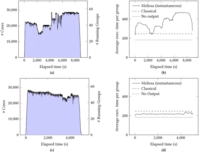
Each Code_Saturne simulation runs on 64 cores. Simulation groups are single batch jobs of 8 MPMD simulations. Thus, each group runs on 512 cores (32 nodes). On the server side, Melissa Server must have enough memory to keep all the updated statistics and to queue the inbound messages from the simulations, and must compute the statistics fast enough to consume the data faster than they arrive. Otherwise, Melissa Server inbound messages queue will end up full, eventually blocking the simulations. We ran a �rst study with Melissa Server running on 15 nodes (240 cores) and a second one with 32 nodes (512 cores) (Fig.6).
For comparison, we also measured the average (over 10 runs) Code_Saturne execution time of a single simulation running on 64 cores without generating any output (labeled as no output in Fig.6). This gives a reference time of the best time Code_Saturne can achieve.
0 20 40 60 # Running Gr oups 0 2,000 4,000 6,000 8,000 0 10,000 20,000 30,000 Elapsed time (s) # Cor es (a) 0 2,000 4,000 6,000 8,000 0 200 400 Elapsed time (s) Av erage exe c. time per gr
oup Melissa (instantaneous)Classical No output (b) 0 20 40 60 # Running Gr oups 0 2,000 4,000 0 10,000 20,000 30,000 Elapsed time (s) # Cor es (c) 0 2,000 4,000 0 200 400 Elapsed time (s) Av erage exe c. time per gr
oup Melissa (instantaneous)Classical No Output
(d)
Figure 6: Two sensitivity analysis en Curie. The �rst one ran Melissa Server on 15 nodes (top plots (a) and (b)), the second ran with Melissa Server on 32 nodes (bottom plots (c) and (d)). Left: evolution of the number of running simulation groups (and number of cores used) during the experiment. Right: average execution time of the running simulation groups during the experiment.
We also evaluated the average execution time (over 40 jobs) when running 8 simultaneous simulations, each one writing its outputs to the Lustre �le system through the Code_Saturne EnSight Gold output writer (using MPI I/O). This gives an optimistic performance for running this study with intermediate �les (labeled as classical in Fig.6). On average a classical execution is 35.3% slower than a no output one. A lower performance is very likely if, as in our experiment, 448 simulations (56 groups) run concurrently.
The �rst study took 2h30 wall clock time, 56487 CPU hours for the simulations and 602 CPU hours for the server (1% of the total CPU time). Simulation groups do not start all at once, but when the resources requested by the batch scheduler become available. At the peak, 56 simulation groups were running simultaneously, on a total of 28912 cores (Fig.6a).
The second study took 1h27 wall clock time, 34082 CPU hours for the simulations and 742 CPU hours for the server (2.1% of the total CPU time). At the peak, 55 simulation groups were running simultaneously, on a total of 28672 cores (Fig.6c). Each Melissa Server process received an average of about 1000 messages per minute during these peaks. Memory usage is about 491GB on the server side, or 15.3GB per node.
In the �rst experiment, the number of concurrent simulations was too large, producing data at a rate that the Melissa Server running on 15 nodes could not process (Fig.6aand6b). The simu-lation groups were suspended up to doubling their execution time. Z���MQ allocates bu�ers on the client and server side to absorb performance �uctuations. It suspends the simulations when bu�ers are full (blocking sends), what happened during this �rst exper-iment. In the second experiment, we ran Melissa Server on 32 nodes giving enough resources to fully remove this bottleneck. The average execution time per group goes below the classical time (Fig.6cand6d). Increasing the number of server nodes from 15 to 32 (about 1% of extra resources as up to 28000 simultaneous cores are used just for the simulations), reduced the burned total CPU hours by 40%. Speed-up is about 1.72 (beware that this direct comparison of wall clock times is biased as the batch scheduler did not allocate exactly the same amount of resources for both cases). To avoid this bottleneck, a conservative estimate on the number of server nodes, based on the availability of a large portion of the machine, is reasonable as Melissa Server requires only a small fraction of nodes (about 1.8% in our case). To further reduce the risks of e�ciency losses, we plan to dynamically limit the number
of concurrent simulations if simulation times go beyond a given threshold.
During this study, Melissa Server treated 48 TB of data coming from the simulations. In a classical study, all these data would be output to the �lesystem, and read back to compute statistics.
Avoiding intermediate �les improves the simulation execution times. When running Melissa Server with 32 nodes, simulations ran on average 13% faster than the classical case, and 18.5% slower than the no output case (Fig.6d). A two-phase algorithm �rst bu�ering the simulation outputs to fast storage like burst-bu�ers or NVRAM before to compute Sobol’ indexes, would still be slower than our one-pass approach that overlaps simulations and Sobol’ index com-putations.
5.4 Fault Tolerance
Fault tolerance was evaluated with the same use case and 32 nodes allocated to Melissa Server.
Unresponsive simulation groups are properly detected by Melissa Server after the timeout is met (set to 300s). They are signaled to the launcher that kills the groups if still running and resubmits them. Once running, the data from the iterations already processed are properly discarded by Melissa Server. Meanwhile, Melissa Server proceeds, updating Sobol’ indices from the messages received from all other running groups. The management of group faults has a negligible overhead beside the cost of recomputing the iterations already processed (can be reduced if the simulations are fault toler-ant).
Melissa Server regularly checkpoints its internal state, consisting of the Sobol’ indices current values and the list of currently running simulation groups with the last timestep received. Each process of the Melissa Server independently saves one checkpoint �le to the Lustre �le system (959MB per process for a total of 491GB for our use case). On average checkpointing takes 2.75s per process with a 1.10s standard deviation. With a checkpoint performed every 600s, the server execution time increases by about 0.5%. Notice that during checkpoints Melissa Server does not process any incoming message. But simulation groups can still proceed with transferring data to the server as long as Z���MQ bu�ers allocated on the client and server side are not full. On restart, Melissa Server takes an average of 7.24s per process to read the checkpoint �les with a 3.21s standard deviation (all 512 server processes concurrently read their corresponding �le). The launcher starts the server recovery process after the timeout expires (set to 300s). It �rst kills all running simulations, and then sends to the batch scheduler a request to start a new Melissa Server instance and a new set of simulation groups. The Melissa Server job being relatively small, the batch scheduler restarted it in less than 1s for all tests performed.
5.5 Data Visualization and Interpretation
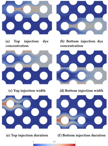
In this section we interpret the Sobol’ indices computed during the experiments. Figure7presents six spatial �rst order Sobol’ maps extracted from the ubiquitous indices. Using ParaView we have chosen a timestep and performed a slice on a mid-plane aligned with the direction of the �uid. The chosen timestep belongs to the last temporal part of the simulation (80thtimestep over 100).
Looking at these �gures an analyst can deduce several things:
(a) Top injection dye
concentration (b) Bottom injection dyeconcentration
(c) Top injection width (d) Bottom injection width
(e) Top injection duration (f) Bottom injection duration
Figure 7: First order Sobol’ index maps on a slice of the mesh at timestep 80. The left column corresponds to the Sobol’ indices for the upper injector while right corresponds to the bottom injector. All maps are scaled between zero (blue) and one (red).
Figure 8: Variance map at the 80thtimestep
(1) The three parameters that de�ne the behavior of the upper injection have no in�uence in the lowest half part of the simulation domain (Fig.7a,7cand7e). Respectively, the parameters of the bottom injector do not in�uence the upper part of the simulation (Fig.7b,7dand7f). These are very coherent results as it indeed corresponds to what happens in the simulation where the dyes are transported from the injectors on the left to the outlets on the right.
Gravity is not used in this case, so we have a symmetry in the behavior of the parameters.
(2) The width of the injections in�uence locations far up or down in the domain (Fig.7cand7d). This is easily understood when imagining the extreme cases. When the width is very small all dye �ows to the right while very few will go up and down. On the opposite, when the injector is at its maximal aperture, dye can easily �ow to extreme vertical locations.
(3) The Sobol’ maps for the duration of the injection (Fig.7e
and7f) can be understood by thinking about the temporal evolution of the simulation. When the simulations are just started, they all inject dye and the duration models when this injection is stopped. Figure7represents a state near the end of the simulation. Thus, it is not surprising that this parameter does not in�uence the right part of the domain (where all simulations were injecting dye) while it strongly in�uences the left side (where some simulations stopped injecting while others continued).
(4) Finally, the dye concentration mostly in�uences the ar-eas were the other parameters have less in�uence, that is to say the center of the top and bottom channels, and the right side of the �ow (Fig.7aand7b).
We recommend co-visualizing Sobol’ indices with the variance of the whole model output; Figure8shows this variance map for the Sobol’ indices presented in Figure7. One of the reasons of this co-visualization is that Var (Y ) appears as a denominator in Eq. (1), consequently when Var (Y ) is very small or zero, the Sobol’ indices have no sense due to numerical errors or can even produce a zero division. Furthermore, it is not conceptually interesting to try to understand which input parameters in�uence low variance areas of the simulation once we know that ’not much happens’ in these areas.
Once �rst order Sobol’ indices are visualized and interpreted we calculate 1 (S1+ ... +Sn), which gives us an indication of
the importance of the interactions among parameters; this is a valuable information that helps understanding how ’independent’ are parameters among them. In our use case, it reveals very small interactions, which means we can just focus on interpreting the �rst order Sobol’ indices. We consequently do not need to study the Total indices as the information they convey is, in this case, redundant with the �rst order indices.
Note that for an unsteady �ow computation, where similar �ow structures could be slightly time-shifted between simulations (in addition to space-shifted), caution must be taken to analyze spa-tial values having a valid interpretation in a time-independent or integrated sense, such as minimum or maximum values, or time during which a value is above or below a given threshold, rather than instantaneous values.
6 RELATED WORK
The usual way to deal with functional outputs (as a temporal func-tion, a spatial map or a spatio-temporal output) was to limit the analysis to several probes in the temporal/spatial domain [47]. Some authors have recently proposed the generalization of the concept of Sobol’ indices for multidimensional and functional data [17] by
synthesizing all the sensitivity information of the multidimensional output in a single sensitivity value. Other authors have considered the estimation of Sobol’ indices at each output cell (see [33] for an overview on this subject). Applications of these techniques on environmental assessment can be found for example in [19,31] for spatial outputs and in [30,32] for spatio-temporal outputs. All these works have shown that obtaining temporal/spatial/spatio-temporal sensitivity maps leads to powerful information for the analysts. Indeed, the parameter e�ects are localized in time or space, and can be easily put in relation with the studied physical phenomena.
Iterative statistics are also called one-pass, online or even parallel statistics as statistics can be computed through a reduction tree. Iterative variance was addressed in [11,15,48]. Numerically stable, iterative update formulas for arbitrary centered statistical moments and co-moments are presented in [7,34] (the one we also use for this paper). These works set the foundation for parallel statistics [35] and a module of the VTK scienti�c visualization toolkit [36]. More recently Lampitella et al. proposed a general update formula for the computation of arbitrary-order, weighted, multivariate central moments [26].
These iterative statistics were used for computing large scale parallel statistics for a single simulation run either from raw data �les [9], compressed data �les [25] or in situ [8]. We also used iterative statistics in an early Melissa implementation to compute the average, standard deviation, minimum, maximum and threshold exceedance for multi-run simulations [44].
Estimation methods of Sobol’ indices are numerous and well-established [38]. An iterative computation of Sobol’ indices has recently been introduced in [18] for the case of a scalar output. In our work, we deal with iterative ubiquitous Sobol’ indices and associated con�dence intervals.
Various packages provide the necessary tools for conducting un-certainty quanti�cation and sensitivity analysis, including support for Sobol’ indices computation, like OpenTURNS [5], UQLab [29], Scikit-learn [37] or Dakota [2]. But to our knowledge, they all rely on classical non-iterative Sobol’ indices requiring a two-pass computation. Thus, all simulation results need to be accumulated �rst, usually in intermediate �les. Some frameworks like Dakota enable to keep all intermediate results in memory. But this is usu-ally unfeasible for computing ubiquitous Sobol’ indices (48TB of intermediate data for our experiment).
Multi-run simulations can also be used to compute surrogate models, also called metamodels, to obtain a low cost but low res-olution model of the original simulation. This surrogate model can later be used for performing a very large number of runs for sensitivity analysis [23]. For particular metamodels, as polyno-mial chaos and Gaussian processes, analytical formulas of Sobol’ indices can be obtained from the metamodel formulas [28]. The HydraQ framework proposes to alleviate the I/O bottleneck when computing surrogate models by storing intermediate �les in burst bu�ers [27].
The parallel client/server infrastructure we adopt is fundamental to the �exibility and reliability of our framework, but is not common on supercomputers, even though such features have been included in the MPI-2 speci�cation. The DataSpace framework proposes a persistent in-memory data staging service where scienti�c simula-tions can dynamically connect and push their results. Dynamics
connections rely directly on RDMA [40]. The Copernicus frame-work for driving multi-run simulations for Molecular Dynamics only needs to support a moderate data tra�c between servers and workers and so can rely on the SSL protocol [39].
Scienti�c work�ows, like Pegasus [12] or Condor [45], or special-ized ones for multi-run simulations like NimRod [1], could certainly integrate our approach, given that they provide the necessary band-width between the server and clients and the needed fault tolerance support.
In situ frameworks like FlowVR [14], Damaris [13], FlexIO [49] or Glean [46], are capable of o�oading analysis to helper cores or staging nodes but only for processing the data of a single simulation (or MPMD run).
7 CONCLUSION
We introduced a novel approach for computing ubiquitous Sobol’ indices from multiple simulation runs without having to store inter-mediate �les. Using this method, statistics are updated on-the-�y as soon as new results are available. Having no need for intermediate storage alleviates the I/O bottleneck and enables to run sensitiv-ity analysis at a much larger scale than previously possible. The combination of iterative statistics with the proposed client/server architecture makes for a �exible execution work�ow with support for fault tolerance and malleable executions.
To our knowledge, the present paper is the �rst work dealing with ubiquitous in transit statistics for a global sensitivity study. Our tests using 8,000 CFD simulations demonstrate that this ap-proach deals with large volumes of data without delaying the exe-cution of multi-run simulations.
Melissa can also be used to compute statistics from large col-lections of data stored on disks. Iterative statistics allow for a low memory footprint and the fault tolerance support enables interrup-tions and restarts.
The experiments presented were performed on a traditional supercomputer. But Melissa architecture also enable executions on less tightly coupled infrastructures in a HTC mode. Simulation groups as well as the server can be scheduled on di�erent machines, given that the bandwidth to the server be su�cient not to slow down the simulations.
There are several directions for improvements that we expect to pursue. The client/server transport layer relies on ZeroMQ. It proved reliable and easy to deploy in an HPC context. However, using RDMAs could certainly take better advantage of the under-lying high bandwidth networks. Data in a simulation group are aggregated using MPI collective communication in an MPMD mode. Resource usage can be improved by performing asynchronous data aggregation towards the server using frameworks like FlowVR [14] or Damaris [13], with the extra bene�t of being less intrusive in the simulation code.
We experimented Melissa with simulation groups only di�ering by their input parameters. Because each simulation groups is a dif-ferent batch job, the framework could start simulation groups using di�erent amount of resources or even using di�erent simulation codes (for multi-�delity or multi-level uncertainty quanti�cations for instance). The di�culty is then on Melissa Server side to prop-erly aggregate the di�erent data for updating the statistics.
Loopback control will also be further investigated. The accumu-lated results on the server side could be used to dynamically control the simulations to launch, through, for instance, adaptive sampling strategies. Such adaptive strategies are particularly useful in un-certainty propagation studies, such as rare event estimation [6]. They are also necessary for the cases of time-consuming large-scale numerical simulations (computer models involving tens of input variables) to build accurate surrogate models to be used for uncertainty and sensitivity analysis. In transit analysis remains a challenge in such a di�cult context.
ACKNOWLEDGEMENT
This work was partly funded in the Programme d’Investissements d’Avenir, grant PIA-FSN2-Calcul intensif et simulation numérique-2-AVIDO. This work was performed using HPC resources from GENCI-TGCC (Grant 2017-A0010610064).
REFERENCES
[1] David Abramson, Jonathan Giddy, and Lew Kotler. 2000. High performance parametric modeling with Nimrod/G: Killer application for the global grid?. In Parallel and Distributed Processing Symposium, 2000. IPDPS 2000. Proceedings. 14th International. IEEE, 520–528.
[2] B.M. Adams, L.E. Bauman, W.J. Bohnho�, K.R. Dalbey, M.S. Ebeida, J.P. Eddy, M.S. Eldred, Hough P.D., K.T. Hu, J.D. Jakeman, J.A. Stephens, L.P. Swiler, D.M. Vigil, and T.M. Wildey. 2014. Dakota, A Multilevel Parallel Object-Oriented Framework for Design Optimization, Parameter Estimation, Uncertainty Quanti�cation, and Sensitivity Analysis: Version 6.0 Theory Manual. Sandia National Laboratories, Tech. Rep. SAND2014-4253 (2014).
[3] Frédéric Archambeau, Namane Méchitoua, and Marc Sakiz. 2004. Code_Saturne: a Finite Volume Code for the Computation of Turbulent Incompressible Flows. International Journal on Finite Volumes 1 (2004).
[4] M. Baudin, K. Boumhaout, T. Delage, B. Iooss, and J-M. Martinez. 2016. Nu-merical stability of Sobol’ indices estimation formula. In Proceedings of the 8th International Conference on Sensitivity Analysis of Model Output (SAMO 2016). Le Tampon, Réunion Island, France.
[5] M. Baudin, A. Dutfoy, B. Iooss, and A-L. Popelin. 2017. Open TURNS: An industrial software for uncertainty quanti�cation in simulation. In Springer Handbook on Uncertainty Quanti�cation, R. Ghanem, D. Higdon, and H. Owhadi (Eds.). Springer.
[6] J. Bect, D. Ginsbourger, L. Li, V. Picheny, and E. Vazquez. 2012. Sequential design of computer experiments for the estimation of a probability of failure. Statistics and Computing 22 (2012), 773–793.
[7] Janine Bennett, Ray Grout, Philippe Pébay, Diana Roe, and David Thompson. 2009. Numerically stable, single-pass, parallel statistics algorithms. In Cluster Computing and Workshops, 2009. CLUSTER’09. IEEE International Conference on. IEEE, 1–8.
[8] Janine C Bennett, Hasan Abbasi, Peer-Timo Bremer, Ray Grout, Attila Gyulassy, Tong Jin, Scott Klasky, Hemanth Kolla, Manish Parashar, Valerio Pascucci, and others. 2012. Combining in-situ and in-transit processing to enable extreme-scale scienti�c analysis. In High Performance Computing, Networking, Storage and Analysis (SC), 2012 International Conference for. IEEE, 1–9.
[9] Janine C Bennett, Vaidyanathan Krishnamoorthy, Shusen Liu, Ray W Grout, Evatt R Hawkes, Jacqueline H Chen, Jason Shepherd, Valerio Pascucci, and Peer-Timo Bremer. 2011. Feature-based statistical analysis of combustion simulation data. IEEE transactions on visualization and computer graphics 17, 12 (2011), 1822–1831.
[10] D.G. Cacuci. 2003. Sensitivity and uncertainty analysis - Theory. Chapman & Hall/CRC.
[11] Tony F Chan, Gene Howard Golub, and Randall J LeVeque. 1982. Updating for-mulae and a pairwise algorithm for computing sample variances. In COMPSTAT 1982 5th Symposium held at Toulouse 1982. Springer, 30–41.
[12] Ewa Deelman, Karan Vahi, Gideon Juve, Mats Rynge, Scott Callaghan, Philip J Maechling, Rajiv Mayani, Weiwei Chen, Rafael Ferreira da Silva, Miron Livny, and Kent Wenger. 2015. Pegasus: a Work�ow Management System for Science Automation. Future Generation Computer Systems 46 (2015), 17–35.
[13] Matthieu Dorier, Gabriel Antoniu, Franck Cappello, Marc Snir, and Leigh Orf. 2012. Damaris: How to E�ciently Leverage Multicore Parallelism to Achieve Scalable, Jitter-free I/O. In CLUSTER - IEEE International Conference on Cluster Computing. IEEE.
[14] Matthieu Dreher and Bruno Ra�n. 2014. A Flexible Framework for Asynchronous In Situ and In Transit Analytics for Scienti�c Simulations. In 14th IEEE/ACM
International Symposium on Cluster, Cloud and Grid Computing (CCGrid’14). IEEE, Chicago.https://hal.inria.fr/hal-00941413
[15] Tony Finch. 2009. Incremental calculation of weighted mean and variance. Tech-nical Report. University of Cambridge. 11–5 pages.
[16] Y. Fournier, J. Bonelle, C. Moulinec, Z. Shang, A.G. Sunderland, and J.C. Uribe. 2011. Optimizing Code_Saturne computations on Petascale systems. Computers & Fluids 45, 1 (2011), 103 – 108. 22nd International Conference on Parallel Computational Fluid Dynamics (ParCFD 2010)ParCFD.
[17] F. Gamboa, A. Janon, T. Klein, and A. Lagnoux. 2014. Sensitivity analysis for multidimensional and functional outputs. Electronic Journal of Statistics 8, 1 (2014), 575–603.
[18] L. Gilquin, E. Arnaud, C. Prieur, and H. Monod. 2017. Recursive estimation procedure of Sobol’ indices based on replicated designs. Submitted, http://hal.univ-grenoble-alpes.fr/hal-01291769 (2017).
[19] D. Higdon, J. Gattiker, B. Williams, and M. Rightley. 2008. Computer model calibration using high-dimensional output. J. Amer. Statist. Assoc. 103 (2008), 571–583.
[20] Pieter Hintjens. 2013. ZeroMQ, Messaging for Many Applications. O’Reilly Media. [21] T. Homma and A. Saltelli. 1996. Importance measures in global sensitivity
analysis of non linear models. Reliability Engineering and System Safety 52 (1996), 1–17.
[22] B. Iooss and P. Lemaître. 2015. A review on global sensitivity analysis methods. In Uncertainty management in Simulation-Optimization of Complex Systems: Algorithms and Applications, C. Meloni and G. Dellino (Eds.). Springer, 101–122. [23] B. Iooss, F. Van Dorpe, and N. Devictor. 2006. Response surfaces and sensitivity
analyses for an environmental model of dose calculations. Reliability Engineering and System Safety 91 (2006), 1241–1251.
[24] A. Janon, T. Klein, A. Lagnoux, M. Nodet, and C. Prieur. 2014. Asymptotic normality and e�ciency of two Sobol index estimators. ESAIM: Probability and Statistics 18 (2014), 342–364.
[25] Sriram Lakshminarasimhan, John Jenkins, Isha Arkatkar, Zhenhuan Gong, He-manth Kolla, Seung-Hoe Ku, Stephane Ethier, Jackie Chen, Choong-Seock Chang, Scott Klasky, and others. 2011. ISABELA-QA: query-driven analytics with ISABELA-compressed extreme-scale scienti�c data. In Proceedings of 2011 Inter-national Conference for High Performance Computing, Networking, Storage and Analysis. ACM, 31.
[26] Paolo Lampitella, Fabio Inzoli, and Emanuela Colombo. 2015. Note on a Formula for One-pass, Parallel Computations of Arbitrary-order, Weighted, Multivariate Central Moments. (2015).
[27] Steven H. Langer, Brian Spears, J. Luc Peterson, John E. Field, Ryan Nora, and Scott Brandon. 2016. A HYDRA UQ Work�ow for NIF Ignition Experiments. In Proceedings of the 2Nd Workshop on In Situ Infrastructures for Enabling Extreme-scale Analysis and Visualization (ISAV ’16). IEEE Press, Piscataway, NJ, USA, 1–6.
[28] L. Le Gratiet, S. Marelli, and B. Sudret. 2017. Metamodel-Based Sensitivity Analysis: Polynomial Chaos Expansions and Gaussian Processes. In Springer Handbook on Uncertainty Quanti�cation, R. Ghanem, D. Higdon, and H. Owhadi (Eds.). Springer.
[29] Stefano Marelli and Bruno Sudret. 2014. UQLab: a framework for uncertainty quanti�cation in MATLAB. In Vulnerability, Uncertainty, and Risk: Quanti�cation, Mitigation, and Management. 2554–2563.
[30] A. Marrel and M. De Lozzo. 2017. Sensitivity analysis with dependence and variance-based measures for spatio-temporal numerical simulators. Stochastic Environmental Research and Risk Assessment, In Press (2017).
[31] A. Marrel, B. Iooss, M. Jullien, B. Laurent, and E. Volkova. 2011. Global sensitivity analysis for models with spatially dependent outputs. Environmetrics 22 (2011), 383–397.
[32] A. Marrel, N. Perot, and C. Mottet. 2015. Development of a surrogate model and sensitivity analysis for spatio-temporal numerical simulators. Stochastic Environmental Research and Risk Assessment 29 (2015), 959–974.
[33] A. Marrel and N. Saint-Geours. 2017. Sensitivity Analysis of Spatial and/or Tempo-ral Phenomena. In Springer Handbook on Uncertainty Quanti�cation, R. Ghanem, D. Higdon, and H. Owhadi (Eds.). Springer.
[34] Philippe Pébay. 2008. Formulas for robust, one-pass parallel computation of covariances and arbitrary-order statistical moments. Sandia Report SAND2008-6212, Sandia National Laboratories 94 (2008).
[35] P. Pebay, D. Thompson, and J. Bennett. 2010. Computing Contingency Statistics in Parallel: Design Trade-O�s and Limiting Cases. In 2010 IEEE International Conference on Cluster Computing. 156–165.
[36] Philippe Pébay, David Thompson, Janine Bennett, and Ajith Mascarenhas. 2011. Design and performance of a scalable, parallel statistics toolkit. In Parallel and Distributed Processing Workshops and Phd Forum (IPDPSW), 2011 IEEE Interna-tional Symposium on. IEEE, 1475–1484.
[37] Fabian Pedregosa, Gaël Varoquaux, Alexandre Gramfort, Vincent Michel, Bertrand Thirion, Olivier Grisel, Mathieu Blondel, Peter Prettenhofer, Ron Weiss, Vincent Dubourg, and others. 2011. Scikit-learn: Machine learning in Python. Journal of Machine Learning Research 12, Oct (2011), 2825–2830.
[38] C. Prieur and S. Tarantola. 2017. Variance-Based Sensitivity Analysis: Theory and Estimation Algorithms. In Springer Handbook on Uncertainty Quanti�cation, R. Ghanem, D. Higdon, and H. Owhadi (Eds.). Springer.
[39] S. Pronk, G. R. Bowman, B. Hess, P. Larsson, I. S. Haque, V. S. Pande, I. Pouya, K. Beauchamp, P. M. Kasson, and E. Lindahl. 2011. Copernicus: A new paradigm for parallel adaptive molecular dynamics. In 2011 International Conference for High Performance Computing, Networking, Storage and Analysis (SC). 1–10. DOI:
https://doi.org/10.1145/2063384.2063465
[40] Melissa Romanus, Fan Zhang, Tong Jin, Qian Sun, Hoang Bui, Manish Parashar, Jong Choi, Saloman Janhunen, Robert Hager, Scott Klasky, Choong-Seock Chang, and Ivan Rodero. 2016. Persistent Data Staging Services for Data Intensive In-situ Scienti�c Work�ows. In Proceedings of the ACM International Workshop on Data-Intensive Distributed Computing (DIDC ’16). ACM, New York, NY, USA, 37–44.
[41] A. Saltelli, K. Chan, and E.M. Scott (Eds.). 2000. Sensitivity analysis. Wiley. [42] R.C. Smith. 2014. Uncertainty quanti�cation. SIAM.
[43] I.M. Sobol. 1993. Sensitivity estimates for non linear mathematical models. Mathematical Modelling and Computational Experiments 1 (1993), 407–414. [44] Théophile Terraz, Bruno Ra�n, Alejandro Ribes, and Yvan Fournier. 2016. In Situ
Statistical Analysis for Parametric Studies. In Proceedings of the Second Workshop on In Situ Infrastructures for Enabling Extreme-Scale Analysis and Visualization (ISAV2016). ACM, 5.
[45] Douglas Thain, Todd Tannenbaum, and Miron Livny. 2005. Distributed comput-ing in practice: the Condor experience. Concurrency - Practice and Experience 17, 2-4 (2005), 323–356.
[46] Tiankai Tu, Charles A. Rendleman, David W. Borhani, Ron O. Dror, Justin Gullingsrud, Morten Ø. Jensen, John L. Klepeis, Paul Maragakis, Patrick Miller, Kate A. Sta�ord, and David E. Shaw. 2008. A Scalable Parallel Framework for Analyzing Terascale Molecular Dynamics Simulation Trajectories. In Conference on Supercomputing. Article 56, 12 pages.
[47] E. Volkova, B. Iooss, and F. Van Dorpe. 2008. Global sensitivity analysis for a numerical model of radionuclide migration from the RRC "Kurchatov Institute" radwaste disposal site. Stochastic Environmental Research and Risk Assesment 22 (2008), 17–31.
[48] BP Welford. 1962. Note on a method for calculating corrected sums of squares and products. Technometrics 4, 3 (1962), 419–420.
[49] F. Zheng, H. Zou, G. Eisnhauer, K. Schwan, M. Wolf, J. Dayal, T. A. Nguyen, J. Cao, H. Abbasi, S. Klasky, N. Podhorszki, and H. Yu. 2013. FlexIO: I/O middleware for Location-Flexible Scienti�c Data Analytics. In IPDPS’13.