Communications in the observation limited regime

Communications in the Observation Limited

Regime

by

Manish Bhardwaj

AUG 0 7 2009 I

LIBRARIES

B.A.Sc. (Honors), Nanyang Technological University (1997)

S.M., Massachusetts Institute of Technology (2001)

Submitted to the Department of Electrical Engineering and Computer

Science

in partial fulfillment of the requirements for the degree of

Doctor of Philosophy in Computer Science and Engineering

at the

MASSACHUSETTS INSTITUTE OF TECHNOLOGY

June 2009

@ Massachusetts Institute of Technology 2009. All rights reserved.

ARCHIVES

Author ... ..

... '. ...

...

Department of El ctrical Engineermg and Computer Science

May 22, 2009

Certified by ...

...

Anantha Chandrakasan

Joseph F. and Nancy P. Keithley Professor of Electrical Engineering

Thesis Supervisor

Accepted by ... . ...

...--- ...

Terry P. Orlando

Chairman, Department Committee on Graduate Theses

Communications in the Observation Limited Regime

by

Manish Bhardwaj

Submitted to the Department of Electrical Engineering and Computer Science on May 22, 2009, in partial fulfillment of the

requirements for the degree of

Doctor of Philosophy in Computer Science and Engineering

Abstract

We consider the design of communications systems when the principal cost is observ-ing the channel, as opposed to transmit energy per bit or spectral efficiency. This is motivated by energy constrained communications devices where sampling the signal, rather than transmitting or processing it, dominates energy consumption. We show that sequentially observing samples with the maximum a posteriori entropy can re-duce observation costs by close to an order of magnitude using a (24,12) Golay code. This is the highest performance reported over the binary input AWGN channel, with or without feedback, for this blocklength.

Sampling signal energy, rather than amplitude, lowers circuit complexity and power dissipation significantly, but makes synchronization harder. We show that while the distance function of this non-linear coding problem is intractable in gen-eral, it is Euclidean at vanishing SNRs, and root Euclidean at large SNRs. We present sequences that maximize the error exponent at low SNRs under the peak power con-straint, and under all SNRs under an average power constraint. Some of our new sequences are an order of magnitude shorter than those used by the 802.15.4a stan-dard.

In joint work with P. Mercier and D. Daly, we demonstrate the first energy sam-pling wireless modem capable of synchronizing to within a ns, while samsam-pling energy at only 32 Msamples per second, and using no high speed clocks. We show that tradi-tional, minimum distance classifiers may be highly sensitive to parameter estimation errors, and propose robust, computationally efficient alternatives. We challenge the prevailing notion that energy samplers must accurately shift phase to synchronize with high precision.

Thesis Supervisor: Anantha Chandrakasan

Acknowledgments

I am indebted to Anantha for his support, encouragement, the freedom to pursue problems, and the collaborative lab environment from which this work emerged. I am grateful to my committee members Dave Forney and Lizhong Zheng for their feedback and encouragement. An extra thank you to Dave, who taught me commu-nications design and coding. I am also thankful to Anant Sahai at Berkeley for his encouragement in pursuing the observation limited setting.

Thanks to my collaborators Pat and Denis! I learnt from both of them, and the thesis is better as a result. Thanks to Vivienne, Maryam, Rana, Amrita and Naveen for being willing movie and dinner partners. Thanks to the many friends who reviewed or helped with this work, including Joyce, Julius, Maryam, Raj and Sashi. Thanks to Rex, Eugene, and Raj - my first friends at MIT! Thank you Kush and Lindi, and Kathleen! Thank you Bill, for your deep commitment to public service, and grinding it out in Bihar!

I would not have made it without Creighton's unwavering friendship, or the love and encouragement of my brother Ashu. How do I thank my parents, Renu and Manoj, for their sacrifices, hard work and love that went in raising Ashu and me? I hope we can lead lives worthy of their love and toil.

This work was funded by DARPA HI-MEMS program (Contract # FA8650-07-C-7704), and in part an IBM Research Fellowship, and a grant from the NSF.

Contents

1 Introduction

1.1 Modeling Energy Consumption . . . . 1.1.1 Transmit versus Receive Energy . . 1.1.2 Sampling versus Processing Energy 1.1.3 Circuit Startup Time ...

1.2 Thesis Contributions ...

2 Coding Under Observation Constraints

2.1 Preliminaries ...

2.2 Fundamental Limits, Relation to Feedback . . 2.3 Traditional Coding ...

2.4 The SPRT with Uncoded Data ...

2.5 Sampling Block Codes When rrx 0 . . . . .

2.5.1 Chernoff's Procedure A ...

2.5.2 Application to Sampling Codes . . . .

2.6 Sampling Block Codes When rrx --- 0 ...

2.6.1 Alternatives to Procedure A . . . . 2.6.2 Application to Sampling Codes . . . . 2.7 Examples of Sampling to Reduce Receive Cost 2.8 Practical Considerations . . . . 2.8.1 VLSI Costs ... .... . 2.8.2 Impact of Non-Zero Transmit Rates . . 2.9 Comparisons with Current Receivers . . . . . 15 ..... . . . 18 ..... . . . 18 . . . . 19 . . . . . 20 23 . . . . . 24 . . . . 25 . . . . 25 . . . . . 28 . . . . 29 . . . . . 30 . . . . 3 1 . . . . . . . . . 31 . . . . . 33 . . . . . 34 . . . . . . . . . . 39 . . . . . . .. . 39 . . . . . . . . . 43 .. . . . . . . 44

2.10 Sum m ary . . . .

3 Synchronization by Sampling Energy

3.1 _{Prelim inaries . . . .}

3.1.1 Energy Sampling Uhannel, Integ

3.1.2 Synchronization Codes . . . . . 3.1.3 Elementary Distance Properties 3.1.4 Performance Analysis . . . . 3.2 Prior Work ...

3.2.1 _{Periodic Sequences . . . .} 3.2.2 Oversampled Sequences . . . . 3.3 Interpolated Sequences . . . . 3.4 Maximum Squared Distance Sequences

3.4.1 Simple, Strong Sequences . . .

3.4.2 Non-Simple MSDs . . . . 3.4.3 Distance Comparison . . . . 3.5 Walking Sequences . . ... 3.5.1 Distance Comparison . . . . 3.5.2 Almost-block w-sequences . . . 3.6 Simulation Results . ... 3.6.1 Low SNR . ... 3.6.2 High SNR ... 3.6.3 Summary of Improvements . . . 3.7 Average Versus Peak Power Constraint 3.8 Summary . ... 3.9 Selected Proofs ... 4 An 4.1 rated Codebooks . . . . . . . 49 .. . . . . . . . 51 . . . . . . . . . . 54 .. . . . . . 56 . . . . . . . 58 .. . . . . . 59 . . . . . . . . . . 61 .. . . . . . . 64 . . . . . . . . . . 7 1 . . . . . . . . . 71 .. . . . 74 .. . . . . . . 76 .. . . . . . 77 . . . . . . 85 . .. . . . . 86 .. . . .. . . . . . . 86 .. .. . . 88 . .. . . 90 .. . . . . . . . 92 . . . . . . . . . . 94 . . . . . . . 95 3.9.1 Chernoff Information of x2 r.v.s as SNR - 0, o . . . . 3.9.2 Bound on Phases in a Simple, Strong MSD Sequence . . .. Energy Sampling Wireless Modem Overview ... ... 97 97 104 109 110 .. . . . 49

4.1.1 Pulsed Ultra-Wideband Signaling ... . . . . 110

4.1.2 Packet Format ... ... . . . . . . . . . . . . 110

4.1.3 Modem Units ... 112

4.2 VLSI Efficient Classifiers ... 113

4.2.1 Suitable Approximations ... . . . . . . ... . 113 4.2.2 Reducing Computation ... . . . . 117 4.2.3 Distributing Computation ... . . . . . . . ... . 119 4.3 Chip Details . . . 120 4.4 Measurements ... ... .. .. 121 4.5 Summary ... ... ... .. 122 5 Conclusions 125 5.1 Open Problems ... ... .125 5.1.1 Coding . . . 125 5.1.2 Information Theory ... 126 5.1.3 Sequence Design ... 127 5.1.4 V LSI . . . . .. . . . .. 129 5.2 Outlook . . . .. . . .. . . . . 130

A Tables of Sequences with Good Squared Distance 133 B Tables of Walking Sequences 139 B.1 Block w-sequences ... ... 139

List of Figures

1-1 Setup of the coding under observation cost problem... .... 16

1-2 Structure of a wireless transmitter and a non-coherent receiver. . . . 18

2-1 The SPRT as decoder for uncoded transmission over the binary AWGN channel ... ... . .. 27

2-2 Receive costs of the rate 1/2 SPRT and K = 7 convolutional code. .. 27

2-3 Performance of the rrx = 1/2, (7,3) code using ME and uniform sam-pling (U) ... .... 35

2-4 Performance of the rrx = 1/10, (7,3) code using ME and uniform sam-pling.. . . . .... ... .. . . . 36

2-5 Performance of the Golay code at rrx = 1/2. . ... 37

2-6 Sampling the Golay code with receive rate 1/6. . ... . 38

3-1 The discrete-time, energy sampling channel . ... 50

3-2 Performance in the low SNR regime with (a) P=2, and each sequence being repeated 16x, and, (b) P=16, and every sequence repeated 64x. 90 3-3 Performance in the high SNR regime (P=2). . ... . 91

3-4 Performance for P=16 in the high SNR regime. . ... 93

4-1 Packet format used in energy sampling modem. Pulse phase scrambling and modulation are not shown. ... 111

4-3 The ML, UVG, and MD classifiers for a (31,16) I-H sequence repeated 32x and lx. The UVG curve lies between ML and MD (32x), and overlaps with ML (lx) ... . . . . . . .. . . . 115 4-4 Impact of SNR mismatch on the MD and UVG classifiers. Dotted

curves denote no mismatch. Curves on the left and right are for 32 and 1 sequence repetition, respectively. . . . ... . . ... 116 4-5 A single-chip energy sampling modem. ... . .. . 121 4-6 Synchronization error rate measured on the chip (courtesy Patrick

Mercier), compared with an unquantized ML implementation (sim-ulated). SNR is the ratio of average power to noise, and not SNR per sym bol. . . . . . . . .. .. ... .. . . . 122 5-1 What does the Pareto frontier look like? ... . .. 129

List of Tables

2.1 Computation required per sample for a brute-force implementation of the ME algorithm. We use II to denote the vector of the M = 2k codeword posteriors, and i* for the index of the observed bit. ... 40 3.1 Best known squared-distances for given nr, P. Sequences in bold are

strong. Subscripts indicate sequence dimension. All sequences without a subscript are simple. (tNo new sequences are listed for nr=6 3 and

P < 8. The distance achieved by I-H sequences is quoted instead.) . . 76 3.2 Block w-sequences for arbitrary P > Pim(t), conjectured to achieve a

distance of 2t. Only non-identity blocks are specified. . ... 85 3.3 Almost-block w-sequences conjectured to achieve a distance of 2t

(ver-ified for P < 16). The first block has length P + 3 and the rest P + 2. Only non-identity blocks are specified. Sequences for P values not included here are in appendix B.2 ... .. 87 3.4 Bounds on sample length for an integer distance of 2t, versus search

complexity (number of candidate sequences) of various families. The t denotes results that are conjectures. . ... 87 3.5 Sequences and their performance in the low SNR regime with P=2.

Rep. denotes number of times a sequence is repeated. ... . 89 3.6 Sequences and their performance in the low SNR regime for P=16. 89 3.7 Performance of sequences in the high SNR regime for P=2... 91 3.8 Sequences and their performance in the high SNR regime for P=16.. 92 3.9 Sequences for the high SNR regime (P=16). . ... 92

3.10 Gains realized when using new sequences in place of O-H sequences. . A.1 Best known squared-distances for given nr, P. Sequences in bold are

strong. Subscripts indicate sequence dimension. All sequences without a subscript are simple ... .... . .. 133 A.2 Sequences that are strong but not simple. All subcodes are shifts, and

sometimes inversions of salt. Subcodes are listed in order from 0 to

P - 1, and specified by the right shift, with an overbar for inversion. 134 A.3 Sequences that are not strong. Subcodes qi are specified by the location

of Is... _{. 135} B.1 Table of block w-sequences. Please refer to section 3.5 for an

explana-tion of the notaexplana-tion. ... ... 139 B.2 Table of almost-block w-sequences of length nr = t(P+2)+ 1. The first

block (bl) has three zeros and the rest have two. Unspecified blocks are identity (see section 3.5.2). ... ... .. . . 140

Chapter 1

Introduction

From an information theorist's perspective, communications design is the quest to equal Shannon's ultimate bound on the rate of reliable communication. From a prac-titioner's perspective, it is building systems that meet specific cost and performance criteria. Sometimes these goals are perfectly aligned, as in deep-space communica-tions. Bandwidth and receiver processing power are virtually unlimited, and the designer's main concern is the severely power limited transmitter on the spacecraft. Massey reckons that every dB in coding gain saved expeditions in the 1960s an esti-mated $1 million [38]!

The huge explosion in wireless terminals has made battery lifetime a critical mea-sure of communications systems performance [11]. Systems designers have a finite bucket of energy, and care about the total electronics energy consumed in the com-munications chain for every bit that is reliably conveyed. When distances or spectral efficiencies are large, the radiated power dominates signal processing power (the lat-ter usually dominated by radio-frequency circuits). In such cases, capacity achieving schemes also maximize battery lifetime [57]. However, such prescriptions fail for a rapidly growing class of short-range, low-spectral-efficiency wireless links, such as re-cently standardized by 802.15.4a[29]. In such systems, the radiated power may be less than 0.1 mW whereas analog and radio-frequency front-ends dissipate 10s of mW. Hence, the traditional theoretical focus on the transmitted power does not yield the most battery efficient solution. Both the circuits and information theory

communi-ties have recognized this mismatch, and issued the same prescription. On the circuits front, it has been recognized that analog signal processing consists of an irreducible component, independent of data rate. Hence, prior work has prescribed increasing data rates to amortize this fixed cost [56, 16]. This is done by increasing the spectral efficiency via higher order modulation, and discarding available degrees of freedom, which is contrary to classical information theory. As constellation sizes grow, the rate dependent component of signal processing power overcomes the irreducible bias, and further increases are not beneficial. Discarding available channel uses makes the transmit signal peakier. Massaad et al. have proved that when the capacity problem is reformulated to account for a power dissipation component that is independent of radiated power, bursty transmission that does not use all available degrees of freedom is indeed capacity achieving [37].

While useful, these prescriptions may have limited mileage in practice. Peaky transmissions are problematic from both a circuit and regulatory viewpoint. For instance, pulsed 15.4a UWB transmitters already operate at the peak power limit imposed by semiconductor technology [58]. Also, supporting multiple amplitude levels may significantly increase the cost of the transmitter and receiver, negating the very premise of these solutions. What options are available to a practitioner when further increases in peak power or higher modulation orders are not possible, but plenty of spare degrees of freedom are available? Are there other approaches that allow trading degrees of freedom or transmit power for better battery efficiency?

We will argue that fundamentally different insights and tradeoffs are enabled by considering a channel that looks like deep-space, but with the role of the transmitter and receiver interchanged. Consider the communications system in figure 1-1.

101... f ± v1

}

W[n] = i.i.d. V (0, O2 = 1)

Figure 1-1: Setup of the coding under observation cost problem.

system uses a code C and BPSK modulation. A procedure P observes noisy channel outputs and infers the information bits. The observation cost is equal to the expected number of samples observed by P to decode an information bit.

Problem 1.1 (Coding under receive cost constraints). What choice of C and P

minimizes the expected cost per information bit under a specified SNR and BER constraint?

Note that the transmitter can send as many coded bits as it desires. What mat-ters is that the receiver judiciously pick the samples it observes. The next chapter deals with this problem in detail. We will see that "receiver" oriented capacity is un-changed, and a conventional capacity achieving code can realize the minimum receive cost. But, the performance versus complexity landscape is dramatically altered, and simple codes with adaptive channel sampling outperform traditional ones. The tech-niques developed here draw from the theory of experiment design, where the number of observations are minimized under a specified reliability constraint by carefully pick-ing from a set of available experiments. These techniques can be applied to different modulation and coding schemes. In comparison, the second part of this thesis consid-ers a particular technique to reduce observation cost - sampling energy rather than amplitude. The key problem turns out to be synchronizing such an energy sampling receiver, and we device new sequences to address this. The last part of our thesis is joint work with P. Mercier and D. Daly, where we demonstrate a single chip, energy sampling wireless modem that incorporates our new synchronization techniques.

In the remainder of this chapter, we discuss sources of energy dissipation in wireless transceivers in detail to see when the formulation above applies. We end the chapter with a preview of our contributions. Three chapters then follow, dealing with coding under observation costs, synchronization of energy sampling receivers, and the energy sampling wireless modem. We end with conclusions and the outlook for this work.

1.1

Modeling Energy Consumption

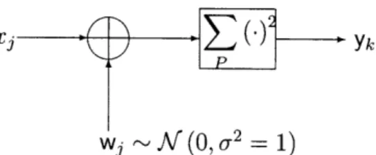
The problem of minimizing electronics energy consumption reduces to that of mini-mizing observation if two conditions are satisfied. First, sampling the received signal should be the dominant source of energy consumption in the communications link. Second, sampling energy must be proportional to the number of samples taken. We now study when these assumptions are valid. Figure 1-2 shows the makeup of an example wireless transmitter and receiver.

bits Encoder

Modulator

II I II II I iGeneration "Ame ' Tx S .Decode _bits L Sampling' Computationi L--- --- L---Cptaon Rx

Figure 1-2: Structure of a wireless transmitter and a non-coherent

receiver.

We divide transmit electronics into signal generation and amplification. The re-ceiver is divided into signal sampling and the subsequent computation. We use SA to denote the electronics energy consumed by component A per information bit. Hence,

stx = Egen + Samp and Erx = samp + Lcomp.

1.1.1

Transmit versus Receive Energy

Of the many factors that determine how Stx and Srx compare, the regulatory limit on output power is usually the governing one. When a high output (radiated) power is permitted, as in wireless LANs, the transmitter is likely to dominate due to Samp.

When regulatory limits are tight, as in UWB systems, the receiver, with its signifi-cantly more challenging signal conditioning and processing, dominates consumption. As an example, Lee, Wentzloff, and Chandrakasan have demonstrated a UWB

system with Stx= 4 3 pJ/bit and Erx=2.5 nJ/bit, i.e. the receiver dominates energy consumption by 60x [33, 58].

1.1.2

Sampling versus Processing Energy

If Srx > Stx, the next question is whether ,samp comp. This comparison is

dif-ficult because notions of complexity, and sources of energy consumption are often markedly different in analog and digital circuits. One prevailing view is that the en-ergy efficiency of digital circuits scales more aggressively than that of analog circuits as technology progresses. Thus the samp/1comp ratio can be expected to grow with

time.

The receiver of Lee et al. quoted above is among the most energy efficient at the data rates of interest to us [33]. Also, virtually all its energy is consumed in sampling. Hence, 2.5nJ/bit is indicative of the limits of energy efficient sampling in current technology. This may be compared with the 0.18 nJ/bit consumed by a recently reported 64-to-256 state, reconfigurable Viterbi decoder [2]. This illustrates that £samp

>

computational burden.

1.1.3

Circuit Startup Time

Whether 8

samp is proportional to the duration of sampling depends on certain

im-portant non-idealities. There are physical and architectural constraints on how fast a sampler can turn on and off. These fixed costs are unrelated to the duration of observation. Cho and Chandrakasan have studied the impact of large startup times on the energy efficiency of sensor nodes, and proposed a new carrier synthesis scheme to reduce it by 6x [15].

Lee et al. have demonstrated a turn-on time of 3 ns in a system with a minimum observation duration of 30 ns. Hence, a proportional model would be appropriate for this receiver. Note that such rapid turn-on is possible due to the carrierless nature of their receiver.

In summary, we detailed a model for energy consumption in wireless devices and the conditions under which sampling cost is a good proxy for the electronics energy consumed per bit.

1.2

Thesis Contributions

Here is a preview of our contributions.

* We have proposed a new class of communications systems where the receiver adaptively samples the channel to minimize observation costs. While motivated by short-range, low-data-rate, pulsed UWB systems, this is, we hope, a useful addition to a modem designer's toolbox, since it allows trading degrees of free-dom for reduced system complexity in a manner that is fundamentally different compared with previous approaches. We hope that future wireless standards will incorporate a "battery emergency" mode that allows the basestation to sacrifice bandwidth to enable a terminal to conserve energy.

* A byproduct of this work is a practical illustration of the power of channel feedback. If the choice made by our adaptive sampling receiver is conveyed to the transmitter via a noiseless feedback link it is possible to breach the cutoff rate over the AWGN channel using the (24,12,8) Golay code. This is the shortest code by an order of magnitude compared with all previously reported schemes, with or without feedback. It is also 7x shorter than Shannon's sphere-packing bound on information blocksize, and illustrates the gains possible when atypical channel behavior is exploited via a maximum entropy sampling scheme.

* We have formally analyzed the problem of synchronization over the energy sampling channel. We have shown that while the distance function of this non-linear coding problem is intractable in general, it is Euclidean at vanishing SNRs, and root Euclidean at large SNRs. We have designed sequences that maximize the error exponent at low SNRs under the peak power constraint, and under all SNRs under an average power constraint. These sequences are

often an order of magnitude shorter than the best previous ones. We believe our work merits another look at the sequences currently used by the 802.15.4a standard.

* In joint work with P. Mercier and D. Daly, we have demonstrated the first en-ergy sampling wireless modem capable of synchronizing to within a ns while sampling energy at only 32 Msamples per second, and using no high speed clocks. In addition to the new synchronization sequences, this required devel-oping computationally efficient VLSI classifiers that are robust to parameter estimation errors. We have demonstrated the inadequacy of traditional, mini-mum distance classifiers for this purpose. It is our hope that this modem will challenge the prevailing notion that energy samplers must accurately shift phase to synchronize with high precision.

Chapter 2

Coding Under Observation

Constraints

We will now study the coding problem introduced in the last chapter. We discuss the connection between this problem and coding for channels with feedback. This is followed by a discussion of the sequential probability ratio test (SPRT) as a simple example of the significant gains possible via intelligent sampling techniques. The more general problem of optimally sampling linear block codes is then discussed. We present simulation results that demonstrate the effectiveness of proposed sampling techniques in reducing observation cost. This is followed by an evaluation of the energy, hardware, and bandwidth costs of the proposed schemes. We end with a comparison of our proposed receivers with those that achieve similar receive cost gains using conventional coding techniques.

2.1

Preliminaries

The adjective 'conventional' refers to a fixed length code that is decoded using a ML criterion. In other words, a codeword is transmitted exactly once, the receiver looks at the entire codeword and uses a ML decoder. Our setup is the binary input, discrete time AWGN channel introduced previously (figure 1-1). Given a (n, k) block code, C, we define the code rate, rc = k/n, and 'SNR per bit', Eb/No = SNR/(2rc). The code

rate must be distinguished from the transmit rate, rtx = k/n', where n' is the total number of bits transmitted for k information bits. In conventional systems, rtx = rc. The r.v. N denotes the number of samples observed prior to stopping. The receive

rate, rrx, is defined analogously to the transmit rate thus, rrx = k/E[N]. Note that,

rrx > _{rtx. The receive cost per bit is defined analogously to its transmit counterpart}

Eb/No, thus, cbit = SNR/(2rrx). For conventional systems, cbit - Eb/No, allowing

easy comparison of receive costs. Note that while stating problem 1.1, we equated cost with the number of samples observed. Our definition here is broader because it allows comparing solutions at different SNRs. The observation cost problem is thus one of minimizing cbit under some combination of pb, rrx, and SNR constraints.

2.2

Fundamental Limits, Relation to Feedback

Shannon's capacity theorem states that for reliable communication,

Eb 22r - 1 No - 2r

where r is the information rate in bits/channel use or bits/dimension. This limit also applies to receive costs as defined above,

22rrx _

Cbit 2_rrx

To see why this is so, note that for every system with a certain receive cost, Cbit, there exists a system with feedback that can achieve the same transmit cost, Eb/No = Cbit.

We just convey the bit that the receiver would like to sample next to the transmitter via the noiseless feedback link. Since feedback does not increase the capacity of discrete memoryless channels [46], the limit on receive cost follows.

A feedback link allows exploiting atypical channel behavior - the receiver can stop early under a favorable draw of the noise process. Receive cost schemes share this trait. They sample just enough to reach the desired reliability. That said, the two problems are not identical. As we just demonstrated, every receive cost strategy

corresponds naturally to a feedback coding strategy. But, a feedback coding strategy does not necessarily translate to a receive cost strategy. Feedback schemes that have full knowledge of channel outputs can "look over the decoder's shoulder" and instruct the receiver to stop sampling once the right result is inferred [45]. This is not possible in our setting, where the transmitter has no knowledge of channel outputs. An example of a feedback scheme that does have a receive cost analogue is decision feedback [21], and we will see that this turns out to be asymptotically optimum under certain conditions.

2.3

Traditional Coding

When an uncoded system operating at a specified SNR cannot achieve a desired error-rate, the simplest option is to use a repetition code, i.e., repeat symbols and then average them at the receiver. A more efficient technique is to use a code. Consider for instance, the setup in figure 1-1 operating at a SNR of 10.5 dB. To achieve a BER of

10-6, we must repeat every symbol twice, i.e., use a (2,1) repetition code. We could

also use a simple (4, 3) parity-check code which also achieves a BER of around 10-6 at this SNR. Hence, we use 4 symbols for every 3 bits instead of 6 - a savings, or coding gain, yc(10-6), of 1.5x (1.7 dB).

A valid question at this juncture is - why not use a capacity achieving scheme like Turbo or LDPC codes with a suitable iterative decoder to achieve the lowest possible receive cost? The reason, elaborated in the following sections, is that the receive problem is governed by a performance versus complexity landscape that is often dramatically different and more favorable when compared with conventional coding.

2.4

The SPRT with Uncoded Data

Fixed length repetition codes offer no gain. However, substantial reduction in obser-vation is possible if we use a decoder with variable stopping times. Consider then a

transmitter that repeats its information bit indefinitely. As Wald demonstrated in the broader context of sequential binary hypothesis testing, the SPRT is the optimum sampling strategy [53, 54].

Definition (SPRT). Consider that m > 1 observations, Yo, Yl,... , _{Ym-1, have been}

made thus far. The SPRT is defined by the following rule,

> A > 0 Accept 01 m-1 m-1 01) If (Yi)= In _{B < 0 Accept 0} 2

i=

i=

p(y 1 )

The SPRT is thus a simple extension of the well-known likelihood ratio test. Instead of observing a fixed number of samples, we stop when the magnitude of log-likelihood exceeds a threshold that reflects the desired confidence. The SPRT is optimum in the strongest possible sense.

Theorem 2.1 (The SPRT is optimum (Wald [55])). Assume that a SPRT yields error

probabilities e1, E2 and expected sample sizes Eo, [N], EB₂ [N] under the two hypotheses,

respectively. Then, any sequential procedure P' that realizes ('1 < E, E' < E2) obeys

E,1 [N'] > Eo 1 [N] and E02 [N'] > EB2 [N].

Since computing log-likelihoods reduces to summation for the case of i.i.d. Gaus-sian observations, implementing the SPRT is trivial for the AWGN channel (figure

2-1). The SPRT requires about a third of the observations used by a fixed length

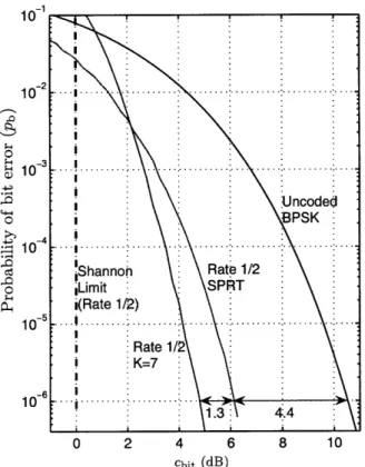
repetition code. This is a significant saving with virtually zero baseband costs. As one might expect, we do not need to repeat the bit indefinitely. There is virtu-ally no performance loss by limiting observations to slightly more than that required by a fixed-length receiver using repetition codes (more on this in a later section). So, how does the SPRT compare with conventional coding techniques? Figure 2-2 plots the receive costs of the 'rate (rrx) 1/2-2 SPRT' and the popular fixed-length

rate (rrx = rtx = re) 1/2, constraint length, K = 7, convolutional code with octal generators [133 171].

InputA '1'

Input-Figure 2-1: The SPRT as decoder for uncoded transmission over the binary AWGN channel.

0 O- 3 I... . . .... -4- - 4 10 7 e Shannon Rate 'Limit SPRT i(Rate 1/2) 0 2 4 6

Figure costs of 2-2: Receive Rate 1/2r

I !K=7 -6 . 10 1.3 0 2 4 6 cbit (dB)

Figure 2-2: Receive costs of the rate 1/2

tional code.

8 10

SPRT and K = 7

convolu-The (2,1,K = 7) code yields a gain of 5.7 dB. The SPRT achieves a gain of about 4.4 dB. Stated in receive cost terms, the (2,1,7) code reduces observation to roughly a quarter, and the SPRT to roughly a third of that needed by a conventional repetition code operating at the same SNR. However, the SPRT has a hardware complexity that is several orders of magnitude lower than the Viterbi decoder for the (2,1,7) code

-10s of gates compared to -10s of thousands [34]. This example illustrates the dramatic

difference in performance versus complexity when coding under receive, rather than transmit cost constraints.

What is the maximum gain possible via the SPRT? The asymptotic expansion of the expected number of samples yields [14],

- In E0

Eo [N] D as rrx -+ 0 (2.1)

where f(x) - g(x) as x -+ a implies limx-a f(x)/g(x) = 1, Pi are the likelihood

functions of channel symbols, and Eo is the probability of error under hypothesis 0. We can now compute the asymptotic sequential gain, ys, by comparing the SPRT's error exponent with that of a fixed-length repetition code. For the binary AWGN channel, we have,

D (N (-a, 0,2) (a, U2))2 D(f (-a, 2) (a, 2

)) =4 = 6 dB (2.2)

YS

D(N(0,O)!

Note that the gain is independent of the underlying SNR. Simulations show that

ys (10-6) for a receive rate of 1/10 is 5.1 dB, about 0.7 dB better than that for rate

1/2, and 0.9 dB short of the asymptotic limit.

A similar analysis can be applied to the binary symmetric channel with probability of error p,

D(B(p) B(1 - p)) 2 for p -* 0

s D(B() B(1 - p)) 4

forp-2 4 _{for p -+}

Here, 13(p) is the (p, 1 - p) Bernoulli distribution. The gain varies from 3 dB for

almost noiseless channels to 6 dB for very noisy ones.

2.5

_{Sampling Block Codes When}

_{rrx -}

₀

The natural way to improve the SPRT's receive cost is to encode the transmitted data.

copies of a codeword drawn from C, a (n, k) code. What sampling procedure minimizes

Cbit under a rrx and Pb constraint?

The problem of choosing from several available coded bits to infer the transmitted codeword is one of optimum experiment design, i.e., classification under a maximum sample size constraint when several types of observations (experiments) are available (see Chernoff's monograph for an accessible treatment [14]). To get some perspective on the intractability of such problems, consider that the optimum solution is not known even for the simpler problem of generalizing the SPRT to more than two hypotheses, with no choice of experiments [20]! We will devote this section to a procedure that is asymptotically optimum (i.e., as rrx -- 0), and the one that follows

to schemes that work well with a moderate sample size.

2.5.1

Chernoff's Procedure A

Chernoff initiated the study of asymptotically optimum design and we now state his central result [13, 14]. In what follows, the set of experiments is denoted by g = {e}. These are 'pure' experiments that form the basis for randomized experiments, whose set we denote by &* . Each element in g* corresponds to a convex composition of the underlying experiments. Likelihoods must be conditioned on not only the underlying hypothesis, but also the experiment. We will use PO;e A p(y 1 ; e). We will also use

a more compact notation for K-L divergence, De(Oi, Oj) ' D(Po,;e

II

Definition (Procedure A). Suppose, without any loss of generality, that the ML

estimate, = 0o, after m observations, y = {yo, , ... , Ym-1}, have been made.

Then,

I. Pick e(m + 1) = arg sup inf De(00, 0) eE&* 0 #o

II. Terminate when min 0o(Y) - £fj(Y) > a.

j¢O

Here, £i(y) is the log-likelihood of of hypothesis 0i, and a is some suitably chosen positive threshold. Thus, roughly speaking, Procedure A picks the experiment that

maximizes the minimum K-L distance between the most likely hypothesis and the remaining ones. Procedure A yields an expected sample size that generalizes (2.1),

- In go

Eo [N]

I

eEg* 0'0

Theorem 2.2 (Procedure A is Asymptotically Optimum [13, 20]). Every sequential

procedure satisfies,

Eo [N] > -n _'Do (l+o(1)) (max co -- 0)

Note that, unlike the SPRT, Procedure A is guaranteed to be optimum only in an order-of-magnitude sense.

2.5.2

Application to Sampling Codes

We denote the codewords of a block code C by {ci, i = 1, 2,..., M}, and the bits of ci by cj, j = 1, 2,..., n. The hypothesis 0i corresponds to ci being transmitted, and the experiment ej, j = 1, 2, ... , n, is defined as observing the channel output corresponding to jth bit.

Suppose next that m observations have been made and 6 = 01, i.e., codeword 1 is the most likely. Then, we define a K-L distance matrix induced by codeword 1,

Do = Dej(01, _Dj O 0i)= D ( Po 1 P) if clj cij

0 otherwise

It follows that if C is linear, then

(Do

}

or replicating certain coordinates increases the coding gain of the resulting codebook. The proof is straightforward and omitted. We believe the converse to be true1. Conjecture 2.1. Uniform sampling is the optimum asymptotic strategy for 'good',

linear block codes, i.e., codes for which no set of coordinate deletions or replications can increase the coding gain.

Uniform sampling achieves,

E [N] - d I

-D(PojI P1)

Normalizing this to the expected observations per information bit gives,

E [N] . -n

k y7cD(Po 1I Pl)

Hence, the overall asymptotic reduction in sampling costs compared with a fixed length repetition code is ycsy, i.e., a product of the coding and sequential gain. Note that the feedback analogue of uniform sampling would be bitwise decision feedback.

2.6

Sampling Block Codes When rrx -

0

In this section, we discuss procedures better suited to moderate sample sizes, and derive a new scheme to sample codes.

2.6.1 Alternatives to Procedure A

Procedure A suffers from two key drawbacks when the expected number of obser-vations is small. First, it relies on a ML estimate to pick an experiment, and this estimate can be very unreliable in the initial phases of observation. This leads to a poor choice of experiments and wasted samples. Second, in picking an experi-ment that maximizes the minimum distance between the ML and other hypotheses,

it completely ignores the a-posteriori probability of those hypotheses. Thus, a highly unlikely hypothesis might dictate the choice of experiment.

In what follows, we denote the a-posteriori probability of a hypothesis by H0, i.e.,

ri0 Pr [E = 0 1 {y}], where E is the true state of nature. Note that we use {y} to denote a set of observations from possibly different experiments. This is to distinguish it from y which refers to samples from the same experiment.

Blot and Meeter proposed Procedure B which incorporates reliability information in distance calculations [7, 39]. Assuming m observations have been made, the next experiment is picked thus,

e(m + 1) = arg max i

HioDe(6,

eag 0

where 0 is the ML hypothesis. Box and Hill proposed a metric that factors in posteriors instead of relying solely on the ML estimate [8],

e(m + 1) = arg max rio, 0[De(', 0) + De(0, 0')] [Box-Hill] 0' 0

Note that in cases where K-L distances commute, the Box-Hill procedure can be written as,

e(m + 1) = arg max E L, 1IoDe(6(' 0)

0' 0

and hence is a straightforward generalization of Procedure B. Chernoff proposed

Procedure M that weighs posteriors more carefully [13],

arg max E rio' [E , 1De(O, 0)/ o, r] [Procedure M]

It is interesting to note that while these procedures yield better results than Pro-cedure A for practical sample sizes, they are either known to be asymptotically sub-optimum, or optimum only under certain constraints [14].

2.6.2

Application to Sampling Codes

The transmitted codeword and its bits are denoted by the r.v.s c and cj,

j

Hi Pr[c = ci {y}] i= 1,2,...,M

7 = Pr[c = 1 {y}= i() Hi j= 1,2,...,n

where Uj(x) is the set of indices of all codewords whose jth bit is equal to x.

A sampling procedure assigns a distance metric, puj, to every coordinate j, and picks the one with the largest metric. We have seen that Procedure A for linear codes leads to uniform sampling, i.e., puA) are identical. Procedure B yields,

(B) = Pr [c

(j I

1 - 7r otherwise

Note that if the a-posteriori probability of the ML codeword exceeds 1/2,

p B) = min ,

1-which implies that Procedure B picks the bit with the maximum a-posteriori entropy. This matches our intuition that the most uncertain bit yields the most information. The more symmetric distance metric of the Box-Hill procedure yields an explicit maximum entropy prescription,

(BH)

Chernoff's Procedure M yields a cumbersome metric,

i(M) = 1i +i(l) 1

which reduces to the Box-Hill metric as the ML estimate becomes more reliable,

(M) (BH)

1P -+ p as max IIi - 1

In summary, all three procedures (eventually) prescribe observing the bit with the largest a-posteriori entropy. We call this maximum entropy (ME) sampling.

There is some precedence of using bit reliabilities in the context of hybrid ARQ schemes for iterative decoders. Shea proposed retransmitting the most unreliable

information bits in order to help the decoder to converge [48]. In our context, this

scheme would essentially reduce to the SPRT. Mielczarek and Krzymien have recently proposed a more elaborate metric to label specific bits "non-convergent" based on forward and backward parameters in the BCJR algorithm [41]. Their scheme does not reduce blocklengths or receiver complexity compared to previous ones, but does reduce the amount of feedback required.

2.7

_{Examples of Sampling to Reduce Receive Cost}

In this section, we report the simulated performance when the uniform and ME strategies are used to sample block codes. In order to quantify the gain due to exploiting atypical channel behavior, we will compare the blocklengths required by our schemes with the lower bound imposed by Shannon's sphere packing bound. We use the numerical techniques in the paper by Dolinar, Divsalar and Pollara [19], which follow Shannon's original derivation [47]. Shannon's derivation permits perfect spherical codes with no constraint on the alphabet. Hence, the bounds are slightly optimistic for our binary input channel.

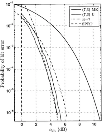
We begin with a simple (7,3,4) dual Hamming code. Figure 2-3 plots the receive costs of this and other rrx= 1/2 codes.

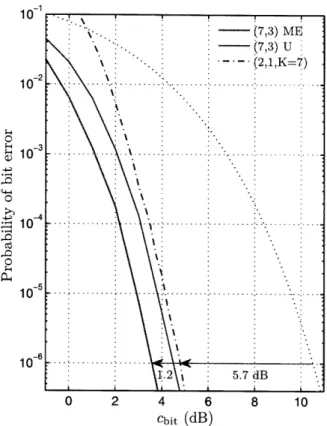
The key observation is that sampling a trivial (7,3) code with rrx = 1/2 using the ME criterion achieves the same receive cost as the much stronger, rate 1/2, K = 7 convolutional code. Figure 2-4 plots the performance for a 1/10 rate. ME sampling

10 S. - (7,3) ME -1 : - (7,3) U S• ... K=7 I .\\ 10 o I O I 1 , i 10-6 . : 0 2 4 6 8 10 Cbit (dB)

Figure 2-3: Performance of the rrx = 1/2, (7,3) code using ME and uniform sampling (U).

has a gain of close to 7 dB, and outperforms uniform sampling by about 0.9 dB. A gain of 7 dB is about the limit of what is possible with convolutional codes using ML (Viterbi) decoding. For instance, increasing the constraint length of a rate 1/2 code from 7 to 9 improves the gain from 5.7 to 6.5 dB. A rate 1/4 constraint length K = 9 with octal generators [463 535 733 745] has a gain of roughly 7 dB. Further rate reductions are unlikely to buy much. Higher gains would require sequential decoding of large constraint length codes [24]. In summary, our receiver achieves, with practically zero baseband processing, the same receive cost as the strongest Viterbi decoded convolutional code.

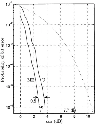
For our next example, we consider the (24,12,8) Golay code, chosen for its remark-able gain at a small blocklength, and its efficient trellis representations. Figure 2-5 plots the receive cost performance of the Golay code at rrx = 1/2. When decoded using the ME criterion, the Golay code achieves a gain of 7.7 dB. This is 0.3 dB from the cutoff limit, which is unprecedented, with or without feedback, for k = 12.

1 0-4 .... .... ... 0-6 10- 6 _.2 5.7 B 0 2 4 6 8 10 Cbit (dB)

Figure 2-4: Performance of the rrx = 1/10, (7,3) code using ME and uniform sampling.

(Note that a fixed-length Golay code has a gain of about 4.5 dB.) The ME criterion outperforms uniform sampling by 0.8 dB, which is significant in this regime. The sphere packing limit on block size at this Eb/No _{and performance is k > 56. For}

comparison, a 3GPP2, rate - 1/2, (768,378) Turbo code achieves a gain of 8.5 dB at a frame error rate (FER) of 10-3

[26]. Crozier et al. have reported a (264,132) Turbo code with a gain of about 7.3 dB at a FER of 10-4.

Other examples include:

* Convolutional: A sequentially decoded convolutional code with K = 41 with a gain of 7.5 dB [42]. Assuming that 5 constraint lengths are sufficient to realize most of this gain, this would be a block size of k - 200.

* Concatenated: A concatenated code with an outer RS(255,223) code, and an inner rate 1/2, K = 7 code. An interleaving depth of just 2 achieves a gain of roughly 7.5 dB. The effective rate is 0.43, and the block size is 3568 bits. (Forney's doctoral thesis is the original reference for concatenated codes [23].

10-1 0 I lO 10- I -6 ... ..

,

7.7

dB

Figure 2-5: Performance of the Golay code at rrx = 1/2.

The example used here is drawn from [19]).

* LDPC: Tong et al. report a (160,80) LDPC code with a gain of roughly 7.3 dB [51]. They also report a (160,80) random binary code with a gain of roughly 7.8 dB. The authors comment that traditional belief propagation incurs a large performance loss (2 dB), and use ML decoding instead, which is computationally prohibitive, limiting the practical utility of these codes.

* Hybrid-ARQ: Rowitch et al. use a high rate, (256,231) BCH, outer code and a Turbo code based on a (3,1,5) recursive systematic convolutional (RSC) code (a rate compatible punctured Turbo (RCPT) code). They are about 0.2 dB better than the cutoff limit for rrx = 1/2 and k = 231 [44]. They also report that an ARQ scheme based on Hagenauer's rate compatible punctured convolutional (RCPC) codes, which uses a (3,1,7) mother code and k = 256, is right at the cutoff limit for a receive rate of 1/2.

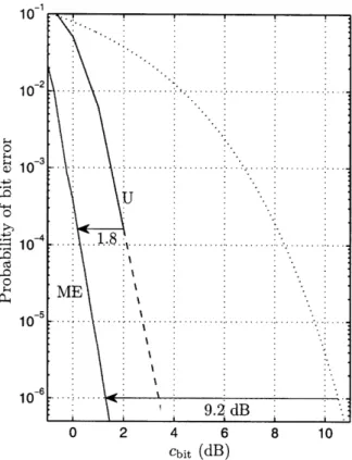
conven-tional codes, including those that use feedback (hybrid ARQ). If we are prepared to lower the receive rate, the advantage is even more pronounced. Figure 2-6 shows the performance when Golay codes are sampled with a receive rate of 1/6.

10 0 1 0 - .. 2 d -. 10 - - I 9.2 dB 0 2 4 6 8 10 Cbit (dB)

Figure 2-6: Sampling the Golay code with receive rate 1/6.

The gain using ME is 9.2 dB, 1.8 dB higher than uniform sampling, and 0.4 dB better than the rate 1/6 cutoff limit. The sphere packing lower bound for this rate and performance is k > 81. Hence, we are close to a seventh of the bound, as opposed to a fifth for rate 1/2. Increasing the expected number of observations expands the

class of atypical channel behavior that sequential schemes exploit, resulting in higher gains.

For comparison, Xilinx Inc. reports a 3GPP2, rate 1/5 Turbo code with block-length k = 506 that achieves a gain of around 9 dB [30]. Gracie et al. calculate the

gain of a rate 1/3, k = 378 code from the same family to be 9.1 dB at a FER of

10-3 [26]. RCPC and RCPT ARQ schemes are ill-equipped to exploit low rates and perform poorly at rate 1/6 [44]. Our scheme outperforms these by about 2 dB.

2.8

Practical Considerations

In this section we determine the energy, hardware, and bandwidth costs of our sam-pling strategies.

2.8.1

VLSI

Costs

We would like the digital baseband implementation of our sampling strategies to consume a small fraction of the energy required to sample the channel. To see if this is the case, we compute the number of arithmetic operations required, and estimate the energy consumed to execute these in current semiconductor technology. This approach has the obvious shortcoming that arithmetic is not the only source of energy consumption. For instance, conveying data, especially over long interconnect, can incur substantial energy costs. However, such estimates are useful in eliminating clearly infeasible approaches, and in declaring others provisionally feasible. It helps that our proposed solutions do not require large memories, interleavers, or switches, as is the case for iterative decoders. This makes our designs more local, and helps reduce interconnect costs.

We assume that the front-end consumes 1 nJ of energy per channel sample [33, 17], and samples are quantized to 3 bits. For a receive rate 1/6 Golay system, we make 72 observations on average, which requires 7 additional bits on top of the 3 bit channel sample, for a total of 10 bits. Hence, we expect codeword log-likelihoods (LLs) to be no wider than this. Simulations by J. Kwong in a 65 nm semiconductor process suggest that 1 nJ allows about 40,000 additions of 10 bit operands (at 0.5 Volt). Measured silicon results by Mercier et al. for a modem in a 90 nm process confirm that these are the right order of magnitude [40]. Ideally, we would like the digital baseband energy dissipation to be limited to 0.1 nJ. This permits at most 4000 10b adds per channel sample. We now discuss the cost of several systems in increasing order of baseband complexity.

We begin with systems that can implement brute-force versions of uniform and ME sampling at negligible cost. Recall that uniform sampling terminates when the

difference between the two largest codeword LLs exceeds a threshold. Hence, for a (n, k = log2(M)) block code, the brute-force strategy requires M additions per

sample to update the codeword LLs, and another M - 1 adds to find the difference

between the winner and runner up, for a total of 2M - 1. As an example, for the (7,3) Hamming code, this is 15 adds per sample, which is clearly insignificant. The (24,12) Golay code on the other hand would require 8191 adds, which exceeds our energy budget by 2x.

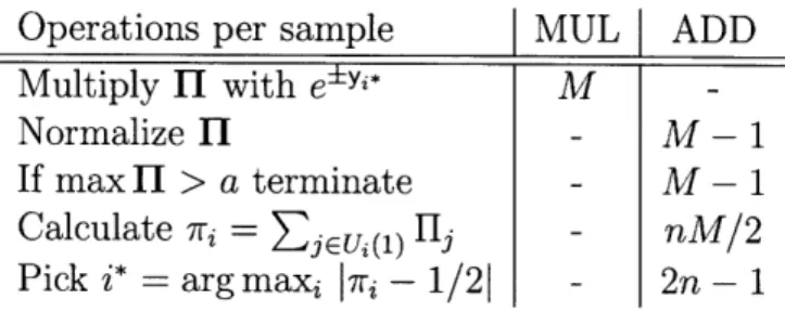
Consider next a brute-force implementation of ME sampling. Table 2.1 shows the computation required to compute bit a posteriori probability (APP).

Operations per sample MUL I ADD

Multiply HI with e±yt* M

-Normalize H - M - 1

If max ]I > a terminate - M - 1 Calculate 7ri = -j vu(1) --j nM/2 Pick i* = arg maxi 7ri - 1/21 - 2n - 1

Table 2.1: Computation required per sample for a brute-force

imple-mentation of the ME algorithm. We use II to denote the vector of the M = 2k codeword posteriors, and i* for the

index of the observed bit.

The table does not include the cost of implementing the exponentiation via an 8-entry lookup table. The (7,3) code sampled using brute-force ME would need about 8 multiplies and 110 adds per sample - again, insignificant compared with the cost of sampling.

Consider next a system that uniformly samples the Golay code. As we've seen, the brute-force approach requires 8191 adds per sample. An alternative is to consider trellis representations of codes (see [24, Chap. 10] for a thorough, tutorial introduction to the general topic.) We use Lafourcade and Vardy's scheme for Viterbi decoding of the Golay code [32], which has essentially the same complexity as Forney's original scheme [22]. The main modification we need is to produce both the winner and the runner up to determine if termination is warranted. We call this the "2-Viterbi" algorithm.

complexity profile {1, 64,64, 1} and branch complexity profile {128, 1024, 128}. Ig-noring branch metric computation, a conventional Viterbi algorithm would require 2 IE| - VI +1 operations (additions and comparisons) to produce the ML path. This would be 2431 for the trellis above. This may be trimmed to 1087 by making the following observation. Roughly put, when a pair of states share two branches that are complements (i.e. c and -), we can halve the adds and the comparisons used in the ACS operation. Finally, the branch metrics may be computed via a slight refinement of a standard Gray code technique, and this requires 84 adds per section. Hence, the standard Viterbi algorithm may be executed using 1087+3x84 or 1339 adds. We have

computed that the 2-Viterbi variation requires 2685+3x84 or 2937 adds.

A more careful analysis reveals that average case costs are lower. We run the 2-Viterbi after every channel observation. If the bit corresponding to this symbol lies,

say, in the third trellis section, we do not have to perform computations for the first two sections. Since we sample bits uniformly, the average number of observations turns out to be about 1852, as opposed to 2937. Next, we always observe the k systematic bits of a block code. Hence, when running a rrx = 1/2 uniform sampling scheme, we incur the 2-Viterbi cost for only half the samples. Hence, the cost per sample is 926 adds. This suggests that we must approach the full cost as rrx -+ 0. But another saving is possible at low rates. When running at say, rrx = 1/6, we

make 6k observations on average. Suppose we observe three channel samples at a time. This incurs a receive cost loss of only 6k/(6k + 3), which is less than 0.2 dB for k = 12, but cuts arithmetic costs to a third, i.e., 2937/3 or 979 adds per sample (not 1852/3, since partial updates are not possible when the sampled bits span more than one section). Note that 1000 adds is a quarter of our energy budget, and this suggests that uniformly sampling the Golay code is energy feasible.

The hardware cost of this scheme would depend on the throughput and latency constraints. A fully parallel implementation would require 2937 sets of 10 bit adders, which, assuming 5 logic gates per single bit adder is not trivial - about 146K gates for adders alone. However, such an implementation could run at an extremely high clock rate, essentially the inverse of the delay of a 30b adder. In current technology,

this can easily approach a GHz or more (depending on the voltage used). Since this is higher than what many systems require, it allows us to reduce the area proportionally. Also, note that observing sets of m bits at a time, reduces throughput requirements by the same factor.

Finally, consider a system that use ME sampling. One way to implement such sampling is to run the BCJR algorithm on the code's trellis [4]. The coordinate ordering for the Golay code that matches the Muder bound is well known, and yields a 24 section trellis with IVI = 2686 states, and IE| = 3580 branches [24]. The max-log-MAP approximation allows replacing the multiply-accumulate (MAC) operations in BCJR with add-compare-select (ACS) operations. Hence, the forward and backward passes have the same computational complexity as a Viterbi pass, which requires 2 JE| - _{IVI + 1, or 4475 operations. Since these passes are run after making a single}

channel observation, we need only partial updates, and the total cost for two passes is only 4475, rather than 2x4475, adds. Unfortunately, the cost of computing the log bit APPs after completing the forward-backward pass is rather high. For a section with e edges, we need e adds each for the branches labeled '0' and '1' respectively (for a binary trellis), and a further e/2 - 1 comparisons per group to find the maximum in each. This is followed by one final subtraction. Hence, we need about 3 IE , or about

10,740 adds. This brings the total to 15,215 adds, which is 4x our energy budget. This computation may be substantially reduced by running a max-log-MAP al-gorithm on the tail-biting trellis of a Golay code, which has IVI = 192 states and

IE| = 384 edges [10]. While the trellis is an order-of-magnitude more compact, the

MAP algorithm needs to be modified to avoid limit cycles or pseudocodewords [3]. Madhu and Shankar have proposed an efficient MAP decoder that avoids these prob-lems by tracking sub-trellises of the tail-biting Golay trellis [36]. Under a plausible assumption about convergence, we have estimated that it takes about five trellis passes, and 2124 adds to compute all the bit APPs. Again, for a rate 1/2 code, this reduces to 1062. We can reduce these further by running the MAP algorithm after groups of observations, though the performance loss in this case is not as easily determined as for uniform sampling. From a hardware perspective, the simplest

im-plementation of this scheme would require about 12 kBits of storage and 6300 gates for the adders. Such an implementation could be run at a frequency limited only by the delay of 32 full adders, again allowing GHz clock rates.

2.8.2

Impact of Non-Zero Transmit Rates

Practical systems cannot afford zero transmit rates. We now determine the maximum transmit rate which preserves most of the gain of our sampling schemes.

The issue of limiting sequential tests to a maximum number of observations was considered by Wald, and his observation essentially answers the question above. Wald considered a sequential test to determine if the unknown mean of a Gaussian r.v. with known variance exceeded a specified threshold. It was shown that limiting the

SPRT's observation to that of a fixed length test, resulted in double the error rate of the latter [54]. A doubling of error is insignificant in the Gaussian context. A mere

fraction of a dB can compensate for this increase when error rates are low.

Proposition 2.1 (Transmit Rate Design Guide). Sequential strategies over the AWGN

channel require (1 + e) more samples than a fixed-length strategy with identical per-formance.

For a SPRT based receiver, this means the transmit rate is marginally lower than that of a repetition coded receiver. Consider next a coded system with uniform sampling. E.g., a (24,12), rrx = 1/6 receiver. A fixed length Golay code provides 4.5 dB of gain. Our scheme provides about 7.4 dB of gain, or 3 dB (2x) more than fixed length Golay. Hence, we require a transmit rate slightly lower than (1/2)(1/6). Simulations show that a rate of 1/14 is indistinguishable from a zero transmit rate.

The idea carries over to ME sampling with the caveat that sampling is intermit-tent. Having sampled a bit, the receiver might have to wait for the next codeword to observe the next desired bit. If a ME scheme selected bit indices independently, we would observe 2 bits per codeword on average. Hence, the transmit rate is reduced by a factor of 2/n compared with uniform sampling schemes. The bit indices are not i.i.d. in practice, and simulations for the Golay code show that only 1.6 bits are observed on