The comparison of available data on PWR assembly thermal behavior with analytical predictions

(1)

J. Liu, N. Todreas

Energy Laboratory Report No. MIT-EL 77-0-09 Draft: June 1977

(2)

(3)

by

J. Liu, N. Todreas

Energy Laboratory and

Department of Nuclear Engineering Massachusetts Institute of Technology

Cambridge, Massachusetts 02139 Topical Report for Task #3 of the Nuclear Reactor Safety Research Program

REFERENCES

..

...

... 41 ... 42 ... 43 ... 43 ... 44 iment ... 45 . ... 45 ... 71 . .. . ... 71 1 Predictions ... 72 ... 75 41

(10)

LIST OF TABLES Page Table 2.1 Table Table Table 2.2 2.3 2.4 Table 2.5 Table Table 2.6 2.7 Table 2.8 Table Table 2.9 2.10 Table 2.11 Table 2.12 Table 2.13 Table Table 3.1 3.2

Parameter Sensitivity Evaluation for

BWR Bundle Sample Problem ... Nine Cases Analyzed in this Study... Four Conditions Analyzed in this Study ... Enthalpy at Location 1.04 Dh after Porous Blockage ...

MDNBR at Location 1.04 D after Porous

Blockage

...

Local Cross Flow for Power Upset Condition.. Local Cross Flow After the Spacer for a

Realistic Condition... Hot Channel Exit Enthalpy for a Realistic Condition... MDNBR for a Realistic Condition ... Axial Distribution of MDNBR for Constant Cross Flow Resistance... Local Cross Flow at Location 6.7 Dh after Blockage for Larger Axial Step Length Case.. Exit Enthalpy at Location 6.70 Dh after

Porous Blockage for Larger Axial Step

Length Case... Exit Enthalpy for Larger Axial Step Length Case...

Test Conditions for G.E. Experiment... Test Conditions for Columbia University

Experiment ... ... 16 17 18 19 20 20 21 21 21 22 23 23 23 47 48

(11)

Table Table Table 3.3 3.4 3.5 Table 3.6 Table 3.7 Table 3.8

Test Conditions for Heston Lab Experiment.... Test Conditions for CEN-Grenoble Experiment.. Test Conditions for Pacific Northwest Lab Experiment ... Comparisons Between G.E. Data and COBRA

Predictions... Comparisons Between G.E. Data and COBRA

Predictions... Ranges of Adjusting Parameters in COBRA

Used by Herbin ... 50 51 52 53 54 55

(12)

LIST OF FIGURES

Page

Figure 2.1 Bundle Geometry of Inlet Flow Upset Case ... 24

Figure 2.2 Figure 2.3 Figure 2.4 Figure 2.5 Figure 2.6 Figure 2.7 Figure 2.8 Figure 2.9 Figure 2.10 Figure 2.11 Figure 2.12 Figure 2.13 Figure 2.14 Figure 3.1

Effect of s/l on Cross Flow Pattern

for Inlet Flow Upset Condition... Effect of s/l on Cross Flow Pattern

for Inlet Flow Upset Condition... Effect of K on Cross Flow Pattern for

Inlet Flow Upset Condition . ... Effect of K on Cross Flow Pattern for

Inlet Flow Upset Condition... Effects of s/l and K on Cross Flow

Pattern for Inlet Flow Upset Condition... Calculation of Channel 4 Exit Mass

Flow Rate Difference Between Case's 1 and 9 for Inlet Flow Upset Condition..

Effect of s/l and K on Local Cross FlowFlow

for Porous Blockage Condition ... Effect of s/l on Cross Flow for Porous

Blockage Condition ... Effect of s/l on Cross Flow for Porous

Blockage Condition ... ... Cross Flow Pattern Generated by Using

the Recommended Values of s/l and K for

Porous Blockage Condition... Sensitivity of Local Cross Flow to s/l

and K for Porous Blockage Condition

(Larger Axial Step Length) ... Test Section Used in G.E. Experiment...

25 26 27 28 29 30 31 32 33 34 35 36 37 56

(13)

Figure 3.2 Figure 3.3 Figure 3.4 Figure 3.5 Figure 3.6 Figure 3.7 Figure 3.8 Figure 3.9 Figure 3.10 Figure 3.11 Figure 3.12 Figure 3.13 Figure 3.14 Figure 3.15 Figure 4.1

Test Section Used in Columbia

University Experiment ... Test Section Used in the Heston Lab

Experiment . ... Test Section Used in CEN - Grenoble

Experiment ... Test Section Used in Pacific Northwest

Lab Experiment... Comparison Between Columbia University

Data and COBRA II Predictions ... Comparison Between Columbia University

Data and COBRA II Predictions ... Subchannel Exit Differential Pressure

(Single Phase) ... Subchannel Exit Differential Pressure

(Two Phase) ... Comparison of CEN-Grenoble Experimental

Data with FLICA code ... Comparison of CEN-Grenoble Experimental

Data with FLICA code... Comparison of Pacific Northwest Lab

Data with COBRA ... Comparison of Pacific Northwest Lab

Data with COBRA ... Comparison of the Normalized Outlet Flow

Distribution as a Function of the Cross

Flow Resistance... Comparison of WOSUB with G.E. Data and

COBRA... Variation of Turbulent Mixing Parameters

with Qyali y for a Flow Rate of 2.44 x 10 kg hr m . ... 57 58 59 60 61 62 63 64 65 66 67 68 69 70 74

(14)

LIST OF APPENDICES

Appendix A Appendix B

Simulation of a Porous Channel Blockage... Cross Flow Resistance Coefficient...

77

(15)

The comparisons of the simplified method with detailed analysis were accomplished in the previous work!1' 1 5 ) It was proved that results obtained by the simplified method are close to those from other more complex methods. In order to have a satisfactory thermal hydraulic analysis method, the comparison between different methods is important but not enough. Check of the results with experimental data

is equally important. The purpose of this study is to compare the physical model and certain empirical constants used in the simplified method to actual data. It should be noted that the model and constants are those of the COBRA family of codes. Chapter 2 treats the crossflow resistance para-meters. Chapter 3 treats the overall two phase flow model.

Few experimental data on the crossflow resistance are available. Therefore, a study of parameters in the trans-verse momentum equation were performed (Chapter 2) to assess the sensitivity of results to their assumed values. Only small effects of these parameters on the overall results can be detected.

Unfortunately, only limited data on core and assembly

(16)

Better understanding of the coolant physical phenomena of an actual multirod bundle which is placed in an actual reactor core is essential to assess the simplified method. Nonetheless, from the available data, it is evident that COBRA which is the tool of the simplified method can predict conditions of single phase and subcooled boiling with nega-tive equilibrium quality (Xe < 0) satisfactorily. It can

not predict the trend under bulk quality condition Xe > 0.02). Even though the bulk quality seldom occurs under normal

PWR operating conditions, a new physical model which can

predict the trend of bulk quality flow for PWR's under severe transients is still needed.

Appendix A is the derivation of the method to simulate a channel porous blockage which was used in Chapter 2.

Appendix B presents the discussion of the cross flow resistance coefficient and the recommended value.

(17)

Chapter 2

CROSS FLOW PARAMETERS SENSITIVITY STUDY

2.1 Introduction

In COBRA IIIC, (2) the transverse momentum equation in-troduces two parameters: s/l and K.

where s/l is the ratio of the gap length to the trans-ition length for the pressure, and

K is the cross flow resistance coefficient without inertial effect.

The COBRA IIIC manual notes that the effects of s/l and K on the results are negligible. This was demonstrated

in the manual by examining the terms in the COBRA IIIC trans-verse momentum equation, and by the results of a BWR bundle sample problem as shown in Table 2.1. In order to confirm or check the above statement, analysis of a two channel geometry using the COBRA IIIC/MIT code with and without porous blockage cases, and another independent case of a six-channel geometry with inlet flow upset condition have been performed with different values of s/l and K.

The results show that the statement that the effects of the two parameters on the results are negligible is generally correct if by results we consider only the

(18)

(1) Under normal operating conditions, the transverse momentum equation does not play very important role. (2) For economic reasons, a comparatively large axial

step length is usually used.

(3) Total cross flow is small even when there is a large local change.

(4) The power difference between channels is not large enough.

The statement that the precise values of s/l and K are not necessary is not correct if we consider results for

local cross flow. Specifically,

(1) The effects of s/l and K on the local cross flow under the inlet flow upset and the porous blockage conditions are large.

(2) The location of MDNBR may change due to the large local change of cross flow.

Nine cases were examined in this study. They represent combinations of three different values of both s/l and K under four different conditions. The values of s/l and K, as well as the assigned case number are shown in Table

2.2. The four different conditions and the number of channels analyzed under each condition are summarized in Table 2.3.

(19)

The method to simulate a channel porous blockage using different values of the spacer loss coefficient is discussed in Appendix A.

The realistic range of K was analyzed in Appendix B. The nominally correct value of s/l was derived in

Re-ference 3.

2.2 Cases with Inlet Flow Upset

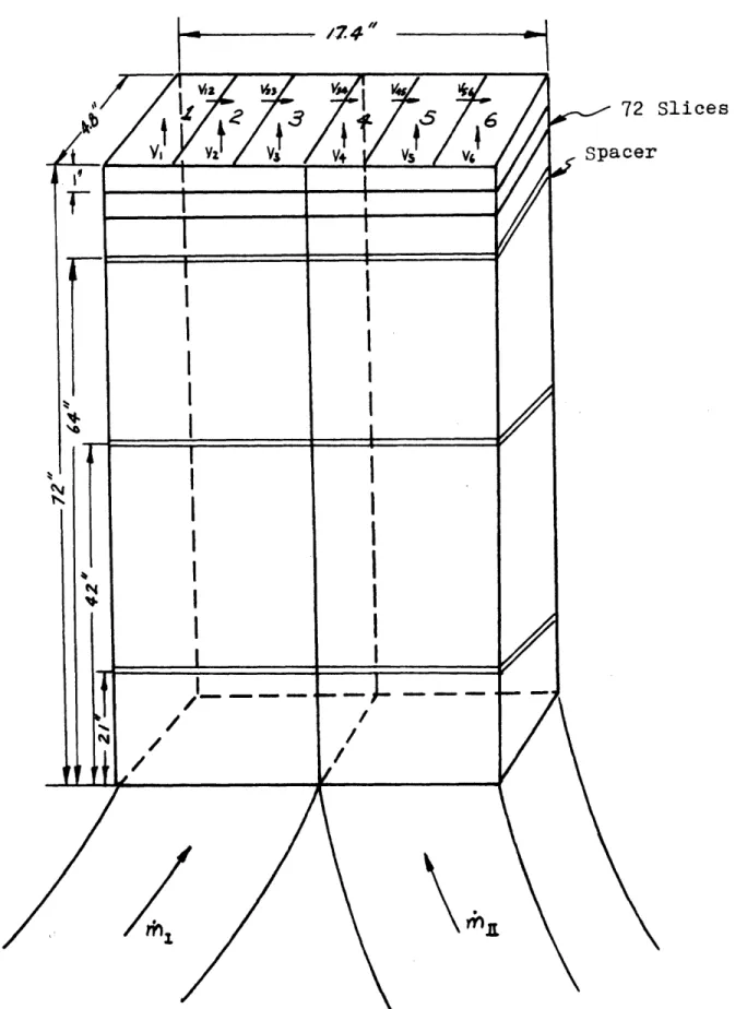
A series of cases of two connected bundles with inlet flow upset and zero power conditions were performed. Fi-gure 2.1 illustrates the geometry of thse two bundles and the location of the three spacers. The ratio of high mass

flow rate m_I to the low mass flow rate mII of 0.75

was selected for the analysis. The two bundles have been divided into six subchannel regions radially and

seventy-two slices axially to ensure a detailed analysis.

The most significant difference due to different values of s/l and K under this condition is the diversion cross

flow between subchannels. The six subchannel model was divided in such a way that the boundary between subchannels 3 and 4 is the actual boundary between the two bundles.

(20)

(See Figure 2.1). Therefore, examination of the analysis results was focused on the cross flow between subchannel's

3 and 4 and these cross flow for nine cases were plotted on Figure's 2.2 through 2.7. The nine cases were obtained by the different combinations of different values of s/l and K as shown in Table 2.2.

The effect of s/1 on the cross flow between channel's 3 and 4 along the axial direction for fixed K can be seen from Figure's 2.2 through 2.4. Three values of K (0.0001, 0.5, 5.0), and three values of s/l (100., 1.3, 0.3) were tested and are indicated on the plot. The effect of s/l is to vary the inertia of the cross flow. For larger values of s/l, the inertia of the cross flow is small

(see cases with s/l = 100.) or vice versa (see cases with s/1 = 0.3). By this we mean that cross flow (with s/l = 100.) changes quicker than those with s/l = 0.3. It seems that the effect of s/l on the local cross flow is independent from different values of K.

The effect of K on the cross flow from subchannel 3 to subchannel 4 along the axial direction for fixed s/l

can be examined from Figure's 2.5, 2.6. The effect of

K is not to vary the inertia but the magnitude of the cross flow. If larger vlues of K (e.g. K = 5.) are used, smaller magnitude of cross flow will be generated, or vice versa

(21)

(e.g. K = 0.0001). The effect of K becomes insignificant for smaller values of s/. For example the differences of cross flow within Case's 3, 6, and 9 (s/ = 0.3 for all three cases) due to different values of K (ranging from 0.0001 to 5.0) is hard to detect. So there is no com-parision plot of these three cases.

From Figure's 2.2 through 2.6, it is clear that the cross flow pattern along the channel varies a lot due to the effects of s/l and K as shown again in Figure 2.7 for extreme Case's 1, 5 and 9.

For fixed s/1 and K (i.e. for fixed case), the five cross flow patterns along the axial direction between

all six subchannels are all alike. This is not surprising, since only one set of values of s/ and K was inputed to the computer code for the five subchannel boundaries.

Because of this similar cross flow pattern, the axial mass flow rate of a certain channel does not change as dramati-cally as the cross flow due to different values of s/l and K. Also, the axial mass flow rate is more important than

the cross flow in determining the overall results.

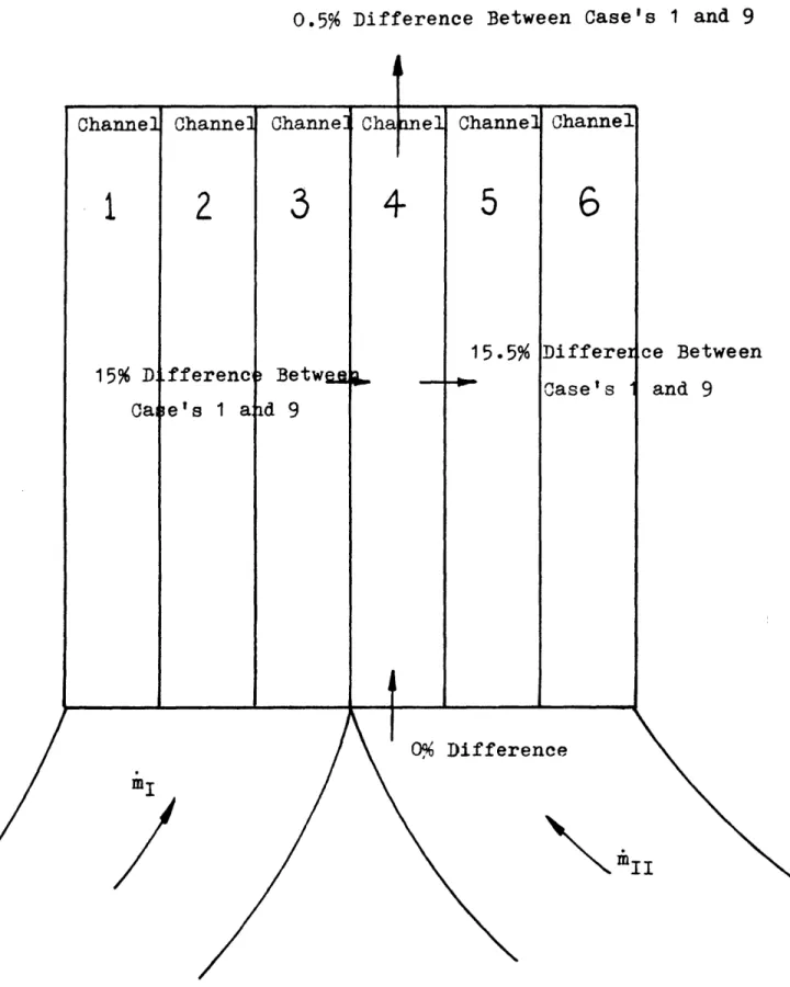
The small difference of channel axial mass flow rate between cases was examined and confirmed by an example. Refere to Figure 2.8, the difference of axial mass

(22)

calcu-lated and compared as follows:

The difference between Case's 1 and 9 of cross flow through channel's 3 and 4 integrated from inlet to the

exit is +15%. The difference between the same two cases of cross flow through channel's 4 and 5 is +15.5%. Due to the compensation of differences, the exit mass flow rate of channel 4 has only 0.5% difference between these two cases.

Therefore, the effects of s/l and K on the overall results are not significant even though the effects on

cross flow are significant under the inlet flow upset con-dition.

2.3 Cases of Channel with Porous Blockage

In order to have a situation such that the transverse

momentum equation plays more important role than under

normal operating condition, a porous blockage with a loss coefficient of 25. was installed at the mid position in one of the two channels. The blockage was simulated in terms of the spacer loss coefficient which is an input parameter to COBRA IIIC code. Details of this simulation are discussed in Appendix A.

Equal channel power input was used to ensure that the cross flow generated could be subscribed to the porous

(23)

blockage condition.

The diversion cross flows at the location just after the blockage for different values of s/1l and K are shown in Figure 2.9. From this figure, it is clear that the effect of s/l on the local cross flow will increase as the value of K decreases. Generally, s/1l and K both have the same order of magnitude effect on the local cross flow. Note that unrealistic values of K and s/1 were

selected in order to investigate the effect of K and s/1l under extreme conditions. Realistic ranges of K and s/l were investigated and discussed in Appendix B and Reference

3 respectively.

The cross flow patterns along the axial direction for nine different cases were plotted in Figurets

2.10,-2.11 and 2.12. The location of the porous channel block-age was indicated at 10.5 inches from the inlet. Also

the value of hydraulic diameter was indicated as D_h on each figure. By comparing these three figures, two impor-tant observations can be made. First, the effect of s/l

on the cross flow pattern is to vary the inertia of the cross flow. Second, the effect of K on the cross flow pattern is to vary the magnitude of the cross flow. Ad-ditionally, the effect of K is insignificant as the value of s/1l becoming smaller. The figures also indicate that

(24)

even though the local cross flow at the location just after the blockage changes considerably from case to case, the magnitude of the total cross flow which is the area under

the curve is very similar. The difference of the total cross flow for two extreme cases (Case's 1 and 9) analyzed is only 3%.

Results of enthaply and NDNBR at the location just

after the blockage for different cases are listed in Table's 2.4 and 2.5 respectively. Since these are a secondary ef-fect of the transverse momentum equation, the differences are small.

The difference of the MDNBR for two extreme cases is the same order of magnitude as the total cross flow

(i.e. 3.4%). Since MDNBR varies linearly with axial flow-rate which for this two channel case varies linearly with total cross flow. Since the channels have equal power, the difference of the exit enthalpy for two extreme cases

is even smaller (0.2% only) than those which have different power.

2.4 Cases of Channel with Power Upset

A power ratio of 1.8 : 0.2 was selected to characterize a power upset situation of the two-channel analysis. No

(25)

s/1 and K on the results of a pure power upset condition. The magnitude of cross flow for the nine cases is

only in the order of 10-31bm/sec ft. The maximum differences of local cross flow between nine cases are shown in Table 2.6. The differences are very small. From this result, no effect of K on cross flow can be detected for the same

value of a/i. The effect of s/l on cross flow is a little more significant than the effect of K.

The hot channel exit enthalpy for the nine different cases are all the same. Because of the same value of exit enthalpy, the same value of MDNBR was generated by the nine

different cases.

The conclusion of this analysis is that the effects of the parameters of s/1 and K is positively negligible for this pure power upset condition.

2 .5 Realistic Cases

A power ratio of 1.2 : 0.8 and a spacer loss coeffi-cient (KG) of 5. Are quite realistic for an ordinary reactor bundle. Based on the above data, analysis was performed

to examine the different results due to different values of s/1 and K.

The effects of 8/1 and K on the cross flow.pattern along the axial direction are quite similar to the cases

(26)

of channel with porous blockage as mentioned in section 2.3. Results of the local cross flow at location just after the spacer are shown in Table 2.7. It can be seen that effects of s/l and K on the local cross flow do have the same order of magnitude.

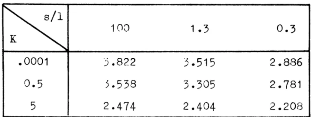
The nine different values of hot channel exit enthalpy and MDNBR are listed in Table's 2.8 and 2.9 respectively. Although the differences are detectable, the differences are insignificant.

Therefore, for a realistic bundle condition, the sen-sitivity to the parameters of s/l and K on the overall results is not significant. Only the location of MDNBR along the axial direction may change from case to case.

2.6 Various Conditions for the Recommended Values of K and s/l

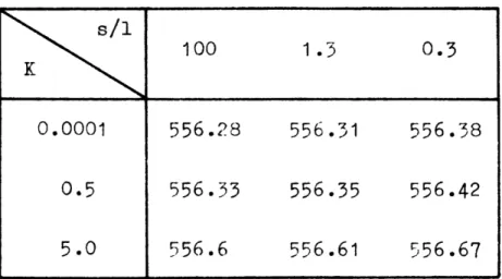
Recommended values of 0.27 and 0.9187 for K and s/1 respectively were utilized to analyze the various conditions mentioned in Section's 2.3, 24, and 2.5.

Figure 2.13 shows the cross flow pattern along the axial direction for the porous blockage condition (i.e. KG = 25., equal power, equal inlet flows). The hot channel

enthalpy and DNBR just after the porous blockage is 556.34 Btu/lb and 4.506 respectively.

(27)

For the power upset condition, (i.e. K_G = ., power ratio = 1.8 : 0.2, equal inlet flow) cross flow is in a

small order of magnitude. The hot channel exit enthalpy and MDNBR is 571.6 Btu/lb and 3.548 respectively.

For the realistic condition, (i.e. KG = 5., power ratio = 1.2 : 0.8, equal inlet flow) hot channel exit en-thalpy of 568.75 Btu/lb and MDNBR of 4.545 were observed.

Comparing all the above results with the results

obtained in the previous sections, only very small differences except for local cross flow can be noticed. This says

that better values of s/1 and K are not necessary for a better overall result except for local cross flow.

27 Effect of Axial Step Length

The flow disturbance due to a porous channel blockage can be detected within a small range around the blockage. This small disturbed flow region, for this degree of block-age studied here, is roughly the same order of magnitude as the channel hydraulic diameter. Therefore, for larger axial step length, the effect on the flow of a porous blockage is small. The sensitivity to s/1 and K under blockage conditions with large axial step length is also small. This can be demonstrated by a case which has the same input parameters as used in Section 2.3 but a larger

(28)

axial step length. It was accomplished by selecting a longer channel (126.7 in) with the same number of axial nodal points.

The results of cross flow at the location just after the blockage as functions of s/1l and K were plotted in Figure 2.14. Comparing Figure 2.14 with Figure 2.9, it is very clearthat the sensitivity to s/l and K is smaller for larger axial step length.

Under this condition, the differences of enthalpy, MDNBR between cases with different s/l and K are even

smal-ler. For example, a typical result of MDNBR along the hot channel for two different values of s/1l is shown in Table 2.10.

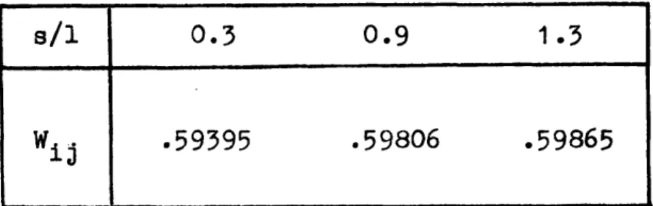
Also cases which have different power input with and without porous channel blockage under large axial step length condition have been analyzed. For a spacer loss coefficient K_G = 5 blockage channel, the results of the local cross flow are shown in Table 2.11. The power ratio

(1.5) was also taken as 1.2 : 0.8. The exit enthapy of hot channel for this case is shown in Table 2.12. It shows that even the case has different power ratio along with a blockage (K_G = 5) located in one of the two channels, the effect of s/l on the overall result is small.

(29)

there is still no change of the exit enthalpy difference as shown in Table 2.13. Therefore, for larger axial step length model, the effects of s/l and K are hard to detect.

This can also be explained by inspecting the finite

difference form of the combined transverse momentum equation: (2)

1 u

s

2u*

m - + -( + ) C +A x

At 6x 1 1 A

where u* is the average of the two subchannel velocities. The relative importance of the terms can be controlled by arbitrarily selecting the axial step lenth x. For larger value of x, the last term is the largest one. The parameter K is contained in the third term. Since this term is small, the effect of K is small. Since the last term contains

(30)

Parameter Sensitivity Evaluation for BWR Bundle Sample Problem Parameter Pressure Ahead of Blockage (psia) G Minimum (o06 lb/hr ft2) Enthalpy 1 ft Down-stream of Blockage

(Btu/lb)

No Blockage

Base Case Blockage

N.t - 1.0

Kj a 0.25 s/ =- 1.0 s/L = 0.25 Ax = 4 inches *= m j Wlj >

u*

a

mn(utu

j )

Table 2.1 (From Table 2 of Ref. 2)

3.50 3.97

3.*5

3.97 3.96 3.99 3.97 3.98 .958 .380 .381 .380 .373 .390 .384 657.72 667.70 667.67 667.74 667.38 668.31 669.92 .423 .423 665.90 668.76

(31)

Table 2.2

Nine Cases Analyzed in This tudy

100 1.3 0.3

.K

.0001 Case 1 Case 2 Case 3

0.5 Case 4 Case 5 Case 6

(32)

Conditions No. of Channels

Inlet Flow Upset

Hight Mass Flow Rate 6

= 0.75 Low Mass Flow Rate

Porous Blockage Loss Coefficent E_G = 25. Power Upset High Power 1.8 2 Lower Power 0.2 Realistic 2 Power Ratio: 1.2 : 0.8 Loss Coefficient: K = 5.

(33)

Channel with Blockage

Channel without Blockage

Table 2.4 Enthalpy ( Btu/lb) at Location 1.04 Dh after Porous 21ockage (KG s/i 100 1.3 0.3

0.0001

556.26

556.24

556.18

0.5 556.22 556.2 556.16 5.0 556.09 556.08 556.06 = 25)

(34)

Table 2.5 vMDNBR at Location 1.04 Dh After Porous Blockage

(K G = 25)

Table 2.6 Local Cross Flow (10- 3 lb/sec ft) for Power Upset Condition

s/1

100

1.3

0.3

K

0.0001

3.07

3.09

3.14

0.5

3.07

3.09

3.14

5 3.07 3.09 3.14

(35)

Table 2.7 Local Cross Flow (lb/sec ft) after the Spacer for a Realistic Condition

Table 2.8 Hot Channel Exit Enthalpy (Btu/lb)

for a Realistic Condition

Table 2.9 MDNBR for a Realistic Condition

K .0001 3.822 .515 2.886 0.5 5.538 3.305 2.781 5 2.474 2.404 2.208 s/i 100 1.3 0.3 K 0.0001 568.52 568.7 569.6

0.5

588.52

568.69

569.04

5

568.58

568.71

568.07 s/l

100

1.3 o.3

K

0.0001

4 585

4.556

4.472

0.5

4.536

4.559

4.478

5

4.590

4.572

4.510

(36)

Distance s/l = 0.3 s/1 = 1.3

IDNBR M1IDNBR

0.0

0.0 7.259

7.166

7.044 6.922

6.801

6.630

6.559

6.43?

6.297

4.082

4.177

4.311

4.428

4.517

4.578

4.616

4.631

4.62-.

4.609

4.575

0.0

7.289

7.166

7.044

6.922 6.801 6.680

6.559 6 .4 9

6.309

4.079

4.185 4.320

4.435

4.523

4.584

4.620 4.635 4.631

4.611

4.578 Location of Porous Blockage (KG = 25.)

Table 2.10 Axial Distribution of DIDNBR for

Constant Cross Flow Resistance K = 0.5

0.0

6.0

12.1

18.1

24.1

30.2

36.2

42.2

48.3

54.3

60.3

66.4

72.4

78.4 84.5 90.5 96.5 102.6 108.6 114.6 120.7 126.7

(37)

Table 2.11 Local Cross Flow (lb/ft sec.) at Location 6.70 Dh

after Blockage for Cases KG = 5., Power Ratio

= 1.2 : 0.8, and Cross Flow Resistance K = 0.5.

Table 2 .12 Exit Enthalpy (Btu/lb) at Location 6.70 Ih after Porous Blockage for Cases KG - 5., Cross Flow Resistance K=0.5, Power Ratio = 1.2: 0.8,

Table 2.13 Exit Enthalpy (Btu/lb) for Cases Power Ratio

= 1.8:0.2, Cross Flow Resistance K = 0.5, No Blockage.

s/1 0.3 0.9 1.3 j ~.59395 .59806 .59865

s/l

0.3

0.9

1.3

Exit Enthalp 642.06 642.05 642.05 (Hot Channel)

s/l

0.3

0.9

1.3

Exit Enthalpy 652.52 652.52 652.52 (Hot Channel)

(38)

Slices

(39)

tm 0 cf I I I ! 1 I CQ a Q CO O( tD

\I

o -A -.b C

0 H

;A l O 1--I/ 1 J

I

. b r iL H. C) cD cD ,/ I

'%\

I1 I I H : D_hd e (D Nj CD 0 0 C+ 0_Ii_Ct 0_Y D CD ' H_ur

0

r9 ! /

0

eN H H CD' HCd 0O I-. I-jCS-d ' W f- C I I I a

(40)

-

-26---

~ .A0 ·

p

0

Co \ ( " t-. am _C CD N HH, CD O -t

O~~~~~~~~~~~~~~~~~~~~~~~~~~~

C.) m 0O H) 0 0 CD co -1 0 CD 0 0 '1 H)₀ H H C) co co Vj

i-

0 CD₍₄ -J. (4 0 4 0 (V I... H ~-_tJ I 1.

0

%_ l c

\

(41)

rA _H ' _S CO CD -0

-t

/ -/ / / / /

I-I/

I I, I

I

M

0

CD I m CD m m (P m ( O 0 \0 0n 0n 0 * . -It P. M, Yl O D I-b o 0 c+ 0 co 0 ts H 0 I-o CD H CD C-0 I--tlj O O O O 0

0

0 CY"

0 -4'

O 0 0 o (D O o_CO ts co H I I I I I

(42)

0

tsz_CD I c+

0

0 C+_O ₀ o x 0 Cd C

w

.

J

,

n

o

So 0

(43)

O CD LtJ o 0 o CO o 0 CD 0 td_C(D L0 H 0 C3 Cd

eI-0

o H' PH I =' r CD *' M O ' _ 0 pq 00

(44)

WV CD ₀ £ (D ¢ I'll 0 -2

0

0 I I i I I I 0 a 0o m m mn cD Ca c 0 0 &>, O o

0

0 o

oIL

r a) 0 Co ,..W

0

l I I

0

Ht) H)_cd C.) tat o Ea p tsl P_o 0 0 CL 0 0om a1₀ o D H 0_cI-_p CD C) 0_Ui H 0_H (D 0 Co_CD d Ea C.

₀

0 cH. H~. 0 0

0

f 1. 1% I I I I I I II o c+ I

(45)

I-0.5% Difference Between Case's 1 and 9

Channel

2

fferenci 3e's 1 a.

Channel

3

BetweA id 9 Cha

anel

I-f

Channel

5 15.5%

-$.-Channel

6

Di fferel

Case's

ce Between and 9

0 a

Differ

mi ence rm]

:I

Figure 2.8 Calculation of Channel 4 exit Mass Flow Rate Difference Between Case's 1 and 9 for Inlet Flow Upset Condition Channel 1 15% D. Cai -II III I ! - w l~~~~~~ I _II ii I -1 L L A

(46)

0 c+ (J uci 3-Z k\ 'I IQm CD 0₀ 0 tD 0 0

r

0 C) (I 0:

(47)

-. .. q · 'F - P tj .* * ~ ~~ ~~~ _ _ __ __ _ _ Cf

o

-0 r Fi) 0 0 CD 0- I -C /

cilr

o 0 0 . 0 I I I I I I I I

~~~~~~~~~~~~~~~~~~~~~~~I

i~~~~~~~~~~~~~~~~~~~~~~~~ o - 0 -~ 0D k~ N n0 - Q o 0 O ·0 i '-3 0 0 0 ,) ., 0

(48)

H :Z

IJ. I

1,14 m --& N) -P- IJ.0 _..c ci.n .

~~-s Y~N C Q c Q > tD C. O CD

ctO

H

-

t

O , CO Ot O C)

, , .

G? CD O c+ O CO 0 0_OC)_o o O 0. O O G?

(49)

_J. D $z Ft O . N W -P 030 C) 0 O o O C0 * 3 C') FJ 0 .o₀ 0 GD H P) TN

~~o ~

~

C. C C3 - cD o co CD oD (D r O -' CD rn0U \91 0 H c F o D U1 '1 H

(50)

C>-ca 0 *o "I O *k *% 4 > 0 0 HO

o e

'd e e OD o Q 0 ¼ o 0 o * c, C a

o

0 c P h. 0e CD 0J H 0_O4 0 0

(51)

CD 0 C O OD H C+D I H* D _c+ 0t 0 0 Q

I-a O

0 0 0 CO 0 0 C 0 0 Co cD m C.) co d m ra II

0

7 L IO TO plj II

0

_OD

0

0 ~r4

-I

(52)

Chapter 3

THE COMPARISON OF AVAILABLE DATA WITH ANALYT I CAL PREDICT IONS

3.1 Introduction

The thermal analysis of open lattice reactor cores requires a detailed knowledge of coolant flow and proper-ties in each fuel assembly. Prediction of these quantiproper-ties is difficult since each assembly is free to exchange mass and momentum with its neighbors. Therefore, sufficient experimental data are necessary to assess the analytical predictions. The ideal way to produce data confidently

is to perform a scaled simulation of a full sized core. Due to the high cost of such a experiment, and the present

lack of facilities, no such experiments have been done. In fact only few measurements have been made in bundle and subchannel test sections.

A survey of published experiments and their compari-sons with analytical predictions was made to assess the COBRA predictions. The assessment was done using COBRA

(53)

3.2 Bundle and Subchannel Experiments

In order to achieve improvement in the prediction by the thermal-hydraulic computer code, it is necessary to gain a better understanding of the coolant flow and en-thalpy distribution in the complex geometries. Five very

completed bundle subchannel experimental works are examined. Comparisons of data with analytical predictions are presented. For detailed information, see References 4 through 8.

3.2.1 Available Data

3.2.1.1 General Electric Data (Data Set 1)

Extensive subchannel test data have been taken in

an electrically heated 9-rod bundle under condition typical

of BWR operating conditions. Uniform and peaked local (radial) power distributions were both selected.(4)

3.2.1.2 Columbia University Data (Data Set 2)

Simultaneous measurements of flow and enthalpy were

made at the exits of two subchannels in a 16-rod electrically heated full-scale model of a typical LWR fuel rod geometry. Experimental data were obtained for conditions of both

(54)

subcooled and bulk boiling.(5 )

3.2.1.3 Heston Laboratory Data (Data Set 3)

Experiments were made to measure the mixing between subchannels in a uniformly heated 7-rod bundle cooled by boiling Freon-12 at a pressure of 155 psia. Modeling water at 1000psia.(6)

3.2.1.4 CEN-Grenoble Data (Data Set 4)

The experiments are performed in the FRENESIE loop with Freon-12. The 4-rod square array bundle was electrically heated.(7)

3 .2.1.5 Pacific Northwest Laboratory Data (Data Set 5) Laboratory experiments were performed to determine the amount of natural turbulent mixing that occurs between two interconnected parallel channels typical of those in rod bundle. An electrically heated test section which simulates channels formed by rods on a square pitch array located next to rods on a triangular pitch array, was used for the experiments.(8)

3.2.2 Summary of the Five experiments

(55)

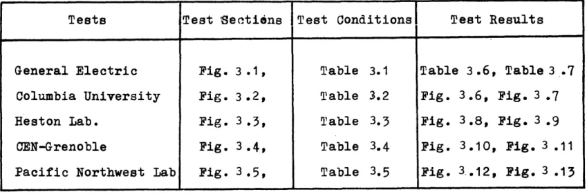
results, the different test sections and conditions are presented. The results shown here are the typical ones

for each experiment. All information in this section is extracted from. References 4 through 8 and are presented either in tables or by figures.

3.2.3 Comparisons of Results with Analytical Predictions The following subsections show only significant ty-pical results. For more detailed results, see references mentioned before.

3.2.3.1 Data Set 1

Table 3.6 shows the single phase data and COBRA pre-dictions with equal to 0.005 and 0.01. For this single

phase condition, predictions do agree with data. Table

Tests Test Sections Test Conditionsl Test Results

General Electric Fig. 3.1, Table 3.1 Table 3.6, Table 3 .7

Columbia University Fig. 3.2, Table 3.2 Fig. 3.6, Fig. 3 .7 Heston Lab. Fig. 3.3, Table 3.3 Fig. 3.8, Fig. 3.9 CEN-Grenoble Fig. 3.4, Table 3.4 Fig. 3.10, Fig. 3 .11 Pacific Northwest Lab Fig. 3.5, Table 3.5 Fig. 3.12, Fig. 3 .13

(56)

3.7 shows the comparison under two-phase conditions between data and the predictions with COBRA for equal to 0.01 and 0.04. Somewhat better agreement is obtained with data for = 0.04. However, the trends in subchannel qualities are not predicted by the COBRA model.

Even with the high mixing, COBRA cannot predict the substantially lower-than-average qualities in the corner subchannel, and higher-than-average qualities in the center subchannel. In fact, if mixing were made infinitely large the three subchannels would all be at average conditions and thus the data cannot be explained in terms of mixing. Therefore, from G.E. data, COBRA fails to predict accurately when the average exit equilibrium quality is greater than or equal to 0.029.

3.2.3.2 Data Set 2

Figures 3.6 and 3.7compare the predictions of COBRA . to the experimentally observed flow distributions in

sub-channel 5 and 11 (Refere to Figure 3.2). These figures indicate that the accuracy of the predicted flow deviation with the homogeneous model is substantially less for condi-tions of subcooled boiling. The agreement is considerably

improved, however, when the Martinelli-Nelson model is em-ployed. This is expected since the Martinelli-Nelson

(57)

two-phase pressure drop multiplier is larger than the homo-geneous multiplier at the same quality. Therefore, mixing

should not be the only effect which needs to be considered to match the data. From this set of data which was performed mainly with subcooled exit conditions, COBRA fails to

pre-dict well when the average exit equilibrium quality is greater than zero.

3.2.3.3 Data Set 3

Figure's 3.8 and 3.9 compares the experimental values of A P12 (exit pressure differences due to inlet flow forced

split) with the predicted values at various of Fm using

HAMBO Computer ode. (9)

Where Fm: An empirical multiplier of mixing coefficient in HAMBO Code.

It can be seen that under one phase condition predictions match data quite well, but predictions can not match data under two phase conditions. The average exit qualities for all cases shown in Figure 3.9 are greater than 0.012. Therefore, the Fm mixing parameter adjustment does not work if the exit average quality is greater than 0.012.

3.2.3.4 Data Set 4

(58)

velocity relative differences versus the mean outlet

thermodynamic quality. Thermodynamic quality distributions between subchannels versus the mean thermodynamic quality are plotted on Figure 3.11. "A" and "KT" indicated on Figure 3 .10 are the adjusting parameters for mixing used in FLICA Computer code. One parameter is for the diffusion of momentum, another one is for the diffusion of enthalpy. Predictions are in good agreement with data when quality is less than zero. But when quality is greater than zero, predictions of subchannel quality can not match data well, even though the prediction of subchannel flow rate matches data. This means that the FLICA code also has trouble to predict accurately for conditions of positive exit equilibrium quality.

3.2.3.5 Data Set 5

Figure's 3.12 and 3.15 are plots of the subchannel enthalpy rise, through the test section and subchannel flow rate versus heat flux for two different channel di-mensions. Each figure represents he exit conditions for a simulated rod spacing, flow rate, and inlet temperature. COBRA calculations are also shown on the plots for compari-son. Good agreement etween data and predictions can be seen from these plots for this two-channel experiment even

(59)

under two phase conditions.

3 .3 Full Scale Core Experimnent

The only attempt to analyze the coolant flow distribution in PWR core from a full scale core experimental data is

the work which was done by Henry Herbin.( 1 0 ) _Assembly

exit temperature distributions are the only data obtained from an actual plant measurements. Parameters in COBRA IIIC were adjusted to match data. The ranges of parameters used by Herbin are shown in Table 3.8. A typical

compari-son of COBRA results with data is shown in Figure 3.14. It can be seen that the assembly exit conditions of the coolant are not greatly affected by the values chosen for each parameter. This low sensitivity indicates that the information obtained from the assembly exit thermocouple can not be used for the determination of the cross flow pattern between the fuel assemblies.

3.4 WOSUB Code

This thermal hydraulic computer code is based on a physical model which includes two-phase separated flow model, subcooled boiling, a vapor mixing diffusion model which accounts for the affinity of the vapor to redistri-bute towards the interior of the bundle, and a recirculation

(60)

loop flow concept model. Louis J. Guillebaud, ( ) based on the General Electric experimental results concluded that this code can predict better than other subchannel

analysis codes under high quality (0.02 0.2) two-phase

condition.

A typical comparison plot between WOSUB, COBRA, and G. E. data is shown in Figure 3.15. The predicted subchannal flow suggests that the WOSUB model has promise to better

match the G. E. data. For detailed information on the WOSUB code see Reference 11. The method is under develop-ment at MIT under Prof. L. Wolf.

(61)

TEST CONDITIONS (p- 1000 psi) Bundle Average Bundle Mass Average Flux Exit

Test G X 10- 6 Power Heat Flux Subcooling Quality

Point (Ib/ft2-h) (kW) (Btu/ft2h) (Btu/lb) i

1 B 0.480 0 0 504.6 1C 0.990 0 0 504.6 1 D 1.510 0 0 504.6 1E 1.97 0 0 504.6 282 0.530 532 225,000 1499 0.029 2B3 0.535 532 225,000 108.7 0.090 2B4 0.535 532 225,000 528 0.176 2C1 1.060 532 225,000 572 0.042 2C2 1.068 532 225,000 35.1 0.075 2D1 0.540 1064 450,000 259.2 0.110 2D3 0.540 1064 450,000 124.4 0.318 2E 1 1.080 1064 450,000 1429 0.035 2E2 1.080 1064 450,000 96.7 0.106 2E3 1.060 1064 450,000 29.1 0.215 2F1 2.07 1064 450,000 59.6 0.040 2F2 2.07 1064 450,000 17.4 0.109 2G1 1.07 1596 675,000 225.9 0.038 2G2 1.080 1596 675,000 189.8 0.090 2G3 1.070 1596 675,000 146.7 0.160 2H1 2.12 1560 660,000 102.6 0.031 2H2 2.12 1596 675,000 59.2 0.099 212 1.06 1880 800X00 227.5 0.104

Experiment Table 2 of Ref. 4

(62)

500 241 1.44 2.U1

500

286

1.43

1.95

500

301

1.48

1.98

500 342

1 .53

2.02

500

325

1.53

2.00

500

305

1.52

1.95

500

290

1.53

2.00

500 270 1.52 1.97 1200 172 0.99 1.01 1200 225 0.98 1.02 1200 277 1.00 1.01 1200 304 0.99 1

.01

1200 329 0.99 1.02 1200 355 0.99 1.03 1200 395 0.97 1.02

1200

420

0.99

1.00 1200

448

1.00

0.99

1200 367 1.47 0.99

1200

350

1.48

0.94 1200

334

1.50

0.99

1200 302 1.51 0.98 1200 245 1.45 1.01 1200 268 1.46 1.01

1200

292

1.45

1.02 1200

313

1.47

0.98

1200 333 1.48 1.00

1200

354

1.48

1.00 1200

378

1.47

0.99 1200

386

1.49

1.00 1200

271

1.48

0.97 1200

278

1.47

0.99 1200

291

1.46

0.97

1200 303 1.48 1.01 1200 316 1.49 1.01

1200

324

1.49

1.02 1200

397

1.52

0.98

1200 406 1.52 1.01

1200

418

1.52

1.00 1200

430

1.52

0.99

1200 441 1.52 1.01 1200 271 1.50 2.02 1200 302 1 .49 1 .98

1200

333

1.50

2.00

1200 367 1.50 2.01

1200

399

1.50

2.02 1200

412

1.50

2.02 1200

424

1.49

2.00 1200

435

1.49

2.02 1200

447

1.49

2.03

1200 455 1.48 2.01 1200 466 1.48 1.99 Table 3.2 1200 430 1.48 2.01 1200 468 1.47 1.96 1200 484 1.48 2.01

1200

$55

1.49

1.97 1200

442

1.50

1.98 1200

430

1.52

2.00

Next Page

Continue

(63)

1200

1200 1200

1200

433

320

225 267 321 391

408

429

453 475 336 352 362 369 381

1.42

1 .8

1.50

1 .45

1.47

1 .43 1 .53 1.46 1 .40 1 .49 2.47 2.44

2.45

2.44

2.43

GAV : Average Mass Velocity

2 . ) , 3. 00

2.99

2.98 3.0O

2.95

2.96

2.98

2.95

2.98

2.97

2.98

2.96

2.97 f (x 0- 6 lb/hr-ft2 )

HIN : Inlet Enthalpy (Btu/lb)

p : System Pres3ure (psia)

Pv : Total Test Section Power (megawatts)

(64)

Where:

Go = whole Q = whole

H1 = inlet

1

channel mass velocity channel power

subcooling

Table 3.3 Test Conditions for Heston Lab. Experiment hr Go Mlb/ft2 0.50 1 .01 1.01 1 .01 1.01 1.52 1.53 1.55 1.54 1.53 2.03 2.01 2.01 2.54 Btu/ 3.75 6.74 18.84 26.99 33.67 12.84 23.82 27.07 31 .78 37.68 14.43 29.22 38.67 19.36 H1 Btu/lb 8.06 '".51 4.34 4.33 4.31 10.93 4.17 4.43 4.35 4.26 11.22 4.42

4.40

11.26

(65)

Outlet absolute pressure: P = 2.3 g/cm2

l4ean mass velocity and inlet temperature: G = 50 g/cm2.s G = 85 g/cm .s Ti

Ii

= 60 a;0 = 60, 65, 70 .

(66)

Pressure

Inlet Temperature

Mass Flow Rates

Rod Spacings Heat Flux

900 psia

330 F (one phase) 510 F (two phase) 1 x 106 lb/hr-ft 2 2 x 106 lb/hr-ft2 3 x 106 lb/hr-ft2

0.020 in

0.084 in

2/3

CHF

Table 3, 5 Test Conditions used in Pacific Northwest

Lab. Experiment

_ __

(67)

SINGLE-PHASE (COLD): MEASURED AND PREDICTED MASS FLUXES

G X 10- 6 G X 10- 6 G2X 10- 6

(Ib/ft2-h) (Ib/ft2-h) (Ib/ft2-h)

Data 0.480 0.311 0.462 COBRA = O.01 0.480 0.352 0.451 COBRA t = 0.005 0.480 0.336 0.447 Data 0.990 0.701 0.939 COBRA8 =0.01 0.990 0.740 0.934 COBRA ( = 0.005 0.990 0.704 0.925 Data 1.510 1.095 1.441 COBRA =0.01 1.510 1.143 1.427 COBRA = 0.005 1.510 1.085 1.414 Data 1.97 1.62 191 COBRA = 0.01 1.97 1.502 1265 COBRA 0.005 1.97 1.424 1847 G3X 10 -(Ibft1-hi 0.526 0.551 0.560 1.150 1.128 1.149 1.690 1.713 1.746 2.19 2229 2273

Table 3.6 Comparisons between G..E. Data and COBRA Predictions Table 8 of Ref. 4 Test Point 1B 1C 1D 1E

(68)

TWO-PHASE: MEASURED AND PREDICTED FLOW AND ENTHALPY DISTRIBUTION Test G X 10' 6 Point (Ib/ft2 -h) G1 X 10 - 6 (Ib/ft2-h) 0.029 Data COBRA P = 0.04 COBRA B = 0.01 0.090 Data COBRA P = 0.04 COBRA P = 0.01 0.176 Data COBRA P =0.04 COBRA P = 0.01 1.080 0.036 1.080 0.106 1.060 0.216 Data COBRA B = 0.04 COBRA 3 = 0.01 Data COBRA , = 0.04 COBRA , = 0.01 Data COBRA/ -( 0.04 COBRA § - 0.01 0.372 0.482 0.491 0.550 0.478 0.454 0.524 0.469 0.417 0950 0.990 0.874 1.046 0.979 0.878 02965 0938 0,826 0.003 0.030 0.046 0.072 0.090 0.104 0.133 0.177 0.194 0.004 0.035 0.057 0.049 0.106 0.125 0.160 0215 0.234 G2 X 10-6 (Ib/ft2-h) 0521 0523 0.516 0530 0.528 0524 0.517 0.526 0.524 1.102 1.082 1.068 1.078 1.073 1.073 1.081 1.044 1.046

Table 3.7 Comparisons between G.E. Data and COBRA Predictions Table 9 of Ref. 4 282 283 284 0.530 0.535 0.535 G3 X 10 - 6 X (Ib/ft2-h) X3 2E1 2E2 2E3 0.014 0.026 0.025 0.076 0.086 0.084 0.180 0.172 0.169 0.026 0.031 0.030 0.097 0.102 0.099 0.185 0.211 0206 0.540 0.552 0.558 0.521 0560 0.571 0560 0.565 0.581 1.162 1.102 1.151 1.180 1.117 1.143 1.126 1.113 1.140 0.030 0.031 0.029 0.104

0.2

0.092 0220 0.178 0.179 0.051 0.038 0.034 0.105 0.109 0.109 0249 0.217 0.220

(69)

Table 3.8 Ranges of Adjusting Parameters in COBRA Used by Herbin

Parameters Range

Axial Node Length 4.2 -7.9 in.

Flow Convergence Factor 0.005 -0.020

s/l Parameter .10 - 0.5

Turbulent MIomentum Factor 0.0 0.9

(70)

Power Peaking

Factors

Subchanns and Peking Pattemrn

Rod Diameter

Radius of Channel Corner Rod-Rod Clearance Rod-Wall Clearance Hydraulic Diameter Heated Length 0.570 inch 0.400 inch 0.168 inch 0.135 inch 0.474 inch 72 inches

Figure 3.1 Test Section used in G. E. Experiment Fig. 60 of Ref. 4

(71)

8 11 I

5

2.363"

Rod Outside Diameter Rod Pitch

Rod to Wall Spacing Rod to Rod Spacing Total Flow Area

Subchannel Area (5, 11) Ratio of Heat Flux

Hot Rods (H) Cold Rods (C) Heated Length 0.422 in 0.555 in 0. 148 in 0.133 in 0.02389 Ft2 0.001168 Ft2 1 t 86% 60.0 in

Figure 3.2 Test Section Used in Colwnbia University Experiment Fig. 1. of Ref. 5 2. s3 ! I r ! 9.

-

·I

-

I

-

r

-

I

-

I· r ·

- -

r r r

(72)

I.

-

f I - :" - -. IX

t.W . O X. '

ki ivC i. , -I : V.-t

(ihOv;); ': 0oC0 1i2.

CF;ZI'D LENOT:E : 16 IN.

CKf;i4EY I(UNMEAri : 4 I1.

Figure 3 .3 Subchannel Division of 7-Rod Cluster Cross Section

... 1

Used in the Heston Lab. Experiment Fig. 1 of Ref. 5.

(73)

'ir

I--

I8

...

Ll'

,17J

IJ,.

I

1I ,I

-

1 43 CAL-f 3.22 co?

Diameter of the rods: 1.072 cm

Distance between axes of rods: 1.43 cm (distance between walls of two consecutive Reduced pitch: 1.333 (reduced pitch in the Distance between rods and walls: 0.358 cm

Center Side Corner Channel Channel Channel Cross Sections cm2 Hydraulic Dia. cm 1.142 1.357 0.829 1.064 0.575 0.874 rods: 0.358 cm) PWR 17 x 17 : 1.325) Total 6.758 1.026 Heating length: 100 cm

Figure 3.4 Test Section Used in CEN- Grenoble Experiment Fig. 1 of Ref. 7 N_N CM RI I I Ih II .00

F~~-

I U

.lII -V Ir I I ro

(74)

H. PJ CD w Ln Io . cD o 0 CD '. 5 * tr X Is. * ₀,4₀ O obZV a 2 O 1Q, Ca A or o 3 rr-_{" as} O 10a t_;b Ca 0 C :r i 0 0 o0 "ft r; o .3₀

6

Cal

a

Pa

v

0

C :r :3

i

0 co O 0 tv 0 a eD a Es 0 h,_to 0 C) F,

v

(75)

+0.15 +0.05 Q 4 U -D -( .05 -o -3 15 25 35 -0.45 -0.20 -0.10 0 +0.10 +0.20 XAV

Figure 3 .6 Comparison between Columbia University Data and COBRA II Predictions (Normalized Channel

Flow Rate Versus Average Quality) Fig. 14 of Ref. 5

I I I G-1XI06 LB/HR-FT2 QAV:0.580XI06 BTU/HR-FT2 P=I200 PSIA .01 0-.01 CHA HOMnoAMOUetS o_ BUoo

MART I NELL I -NELSON

I I I I [ I [ I ! I · ·

-_

_

(76)

+0. 15 +0.05 0 '3 U 0 1u -0.0 -0.15 -0.25 _ i. - . X,, _ . _ -0.35 -j.25 -0.15 -0.05 +0.05 +0.15 XAV

Figure 3.7 Comparison between Columbia University Data and

COBRA II Predictions (Normalized Channel Flow Rate

Versus Average Quality) Fig. 15 of Ref. 5

I I I -I I G=2X10 LB/HR-FT2 QAV=0.580X106 BTU/HR-FT2 D-1'nn oC!, 11 .01 01 1=0 I I I I I I I B I I -~ ~ ~ - -I I I I I I I I . .

(77)

a 2

qi'P ]

[[J [

[

0 .... ~~~~~ "

_b

_o

4 -

0

. · _O~~~~~~~~~~~ i ! , .. -r I₁ ₄ o

i

:

f

F o · ~

--i _4lb_~ _- _! _: _{-, ...} F--.~ . o .Z - - -_ * S~~~~~~~4 I -: I, * -i .. ,{ . _ Is_a .4 a --I rl .4 3 ., i I , o, . o ;, o ... 3 n~3 n t %'-.i I _~IJ _ _ I | ' .4 -- I i. I I _I :· . 4 I . . -A - . . j-4

It

-09 Fl m EE

I

f" -4 hd PO N-) 0o t55

3

la .4

I,

I

i

m 4 0 2 3 r, x -4 0 .4

a

,q I" m

2

-4_* F" , C An a, $A .... sow I a r% I P .; I f i II

(78)

0 3; .4·· · nx .4_.4 q( ~ - 4:r! i· n S. 4. :1;" 4-:- ' '4 ; t . .41 ) as .~4 . -. _ II o_~~~~~r /

7,

!

i

-

I

..

r ,/1,/ /.

., _ s L . _i 0 I4 I _I ' i , 1i r ~ ~ ~ I J

_..

, __ . , I 0 I i .! '4. '

it

',/

_..

_It

/,;.-i i I I _OI ' ,

t

I

i

. I II .I

_.'

44' -

, .p

_

.

·_~ ~~~~~. , , . . a .44. : C. I.. J .. - ' " w hd 014 0 CO ~t_(d Q; ho m (JJ 0 c_W Zo C a

n

2 30

z

m X -n

-Il"

z

:0 r e-IV 'A Cm (A W*1

I-Jf 4,% a ._I S" i ." :3 o n £ 2 . p. - ' I ,₀ '2 I I II I _ a .... k z '_' II1£ ; ! I I II1.-. I - -ql ;, II .i % ;·

(79)

I . I *1 A.. ,I . I . .. -( - -... .. .3 .. 3C i . : . -; .-_ .... .-_i. -i i-h, ... .L.

. .T

I : i. [. ? ' .i. _ i-.C -. I-- , ! ! .. :-... .. -- 1·- :····--:·---1... :. . '' I"` ' '' r... : ;.. :. _{I T}. I _-L_. -I

1. 1

· ·1···-! · · ! · ·: ...-....- ,. ...- 1,.;.... 1 ; `I 1-·-· 1...1.... . _...1.. _.i...;.._!.-.i.-.

i-t--

_

t r·

· fi

- "\

\

-.i::1

I

/ - 'I !. -'i/. .. . 1 I.: ·.

i"

.,-.:"

:

. . I i I. ... . i.. I *i.. .. - ,1 : !.: . - J .. .... .7 ; .._t _ I - -.. - - !iI- _.. I "l i i , 1 . : -: .: I . "' I. I.: - I !; --- > T --. : T i .: 4: . .:: . i --. i I - l *i "-'

-I

L .'-/

'-

:

I _ ,* ,I I. j. ::i :.- .: :. . _~ :::. T .----'-..,-- ~--.. .,.. ..-- T-·! . · . A -- - - L ' ·:: Ji :· . i w . --', '; i-i-i'. ] ; I 1

.i

T :.. , .i l _. , _

.. ,' O . ...

I

D'

l

I

r

t],

'---

LO

: "

_.;

_....

1... j_

₁

_

_i

L " ..

_...

_l

... .. . ..

·J

i

'ij"

i :'':'i,'''

jll '

'

.1 ! '

'i

, " , ...._"i _....

..

Ott L. o

0

oEl H I-i'. CO tq0 CDO O O0 II CD C (D cat 04_so to_Cx ty _ia L.. · T-C-·- 1._ ; 1 .- ·. i I l : '''; ''.'.; ' 1 ''; ' I ... ...- ~ -r .. ... C... w I-¢ ' I' ..4 .._ -... . V. .... ..:... ! :..: i: I ::1 .. . : ! . l' .' . .-'I "' i: i : i: . : :: l?.j .. . :i . ' -a. -_17 . L 1- :i ..::.. i ... -ilS ...

.l..:

j ..-L

. ... ... . .. . t-, .. S:.,.;i. I i i . : i i

· I' I.: :

.[.i..

... .._'J":lI'":'.... .. ...i

t:.J.... ...: or;·

:.!:i.;.'?

'

... ..., ..

...: ..

...

.1-

.

.1.:.

(80)

· · _I·I__·_·_····(___ L·_···__l_ ___··· · C ____( __I _···_ _ ~ ~ · I_ ___·_____ ____ _i_ _·____ ___I ·I __·__ _1-· !--- ... ·: " ! _{". - ."}~... . . ... _{. .'e}' % '-t _- _{.;.. ..}:;.. I I . I r- II - -- il- I i !I : .i ... _.A.A....· .. , . I : ~* _T II

.

:----. ....

I

'

,o

I

-'

· r · \· I .. .. .... : ": ( " : .L.i:::::::: ·LL...-..I I : i --··--·---L-i---·' :"'· : '·" ·--l-1-i.lii; ... I 1 · · · · t··· '"'' ' ".'t':: · ·. : I'.·.I· I·: _ .... ,·. ' . -:"-%'-i ~' ~'-TT. :.. ..-.~__- ·:

-~~~~~~.=·

.i....

'--.-.-i'i · !...'

'

"~

r . .. 4 1 7 -11. _{.: : ! : ::r. I- -;.:} . . .-: I _': , · :1", . ; . T ..;. .::::.: ; · · ' I:·:. 1. :i.r · · · · ·t·· ;1··· ·-: . 7 . ..__ _{;. : .} : :1 ; i : . 7. I ; - : i -:'7 -7':' i - I I I L-- :.-.-1

·i·: I · ·I i· :i

....

' :..!.i.:-~'

_{i'!i '}

· I I '. &. .

j'i~~~~.. .:.'.!-.

~"

-'

i':

~.-,1::

"" _J~! 1_L-·. ':: :.j.: : -'-: .,I.: :.

---

,ir----· m ... - -~- ___ ___ - : k ' il i,--- --. I . ; 'i. I - ' · t .. : ;.. ...

~~~··

'"':'-/ ...f '- , 'i C C~' -:'-.."3 Ca rr O

s

h----..-'-r--~

- u

-

'

6 .

'.-P ...b.. .··x O .o o(ll It It I I i(O

o

ul

_i _t I

i

1' j . .i · I i-·r~l i . . . ' -66-". i I I : i m I. I I i . . J_ . .:.! I i .. I... , 1- T I . --i i i··· _{j..:;_['} I.em. ' · J I . ,'T..-" " ... .--... L . . . i-. :' ...t ,":i -:.i

'F"--"'t""ff··-:

:--·

U-:

...

A ; - ! ·· · __ ···I hd Ott w -A

0

' i" ' -""-' ·· "~: ~'

J.:

;:·::i

:'.:i:i.'.:::"~.

' .. ""~'~C.

X

.

.: .:. r

':_J' :' i ~:

···-

-I . : : i : I .. .J : · .; . · · ; I ' · 0 i- S-, 9 O m ₀ b CDa~o o <1

(1p

C+

₀

0 e 0C 'd Y(bP) 014 C+_CDO C4. -,,,

....-.

I . o. . .· :. .... : I . . '. ;. ' .. -., . - N. . .N I .

:.

..:... i..

: ..

_i :.._1 . 'i i.. i r· _i·

.i. _{-i-l·-·-·-} _{i ·} _·i.

· ·· ---' .: ."::· !.::":'

1·~~~~~~~~~~~,1

...

· · · :

::-

riir

-t : . _{. .. . .0}.. . .·~ r--_'....

r '

- ;·7. -,-= -~C·_/--,.-... ; i r. .· i· ·

:

~ ~ ~/:

.

:

··

.

I

..: .. I

:~~~~~~~~~~~~~~~~~~~...

·.

,:~~~~~~~~~~~~~~~~~~~~~~~~~~~, :: '-·.·-i·..

?~~~~~~~

.-..

i' · .. ,,~.,,'-:4=~- --- .:... . .... i

I1..

...

...

..

-_.-/

: :i:'!- -.' . :- . '... I _r' :: .. . I . . . CI . : : r r·l··i·:: i" · '·:·! -f

* \i

-'it"l-'-A ' ...:

'a

' . I -?'-I4I ·. , .. i : i. :'..i... t-l: :.LLLC.;-L;- fLi-. ·- · ·· -- ~ ... -' :.._ !.%. ; .... · ·':i:'.:l I' F' .-. · .~' i ;. ': .i: :.i.i · 1. :'.. .. ·..

:-:.- _'

:~

:..'":!::: : : : .I i I '" :: · i .. . 1. : . : i· . . : .:-:- il - -. .. _ -,-': /-:' .:.'. i : !"' .' ... . , . . L : -. "," F:-!.-:--1. .: l.. . . j . . I . ' "'I ..

. i.

:. ..

I .. .. I I. ,

·

t .:I:· .,. i.. i: t i ;..i .. . :.. - I . -4, . ! . . ,:: ·. i.iL.,:,i...l.;;I '· - , .' i. 7 ·~ ... ' "''" . -....'

xIl ...

... ~

:..

....

·. i.. _:,~-!..

.."i~~~~~~~~~~~

'

;

· , i .' · i:,.!: .r :' i :-- I ' ' ! ...

.i ...:.,

:: ..

: .

I···:--i· · · -~ . : - . - - . . I . . . ... I : . :. I .: ;. i i -. ! ! i : - : i I I i_I I " 1 tA~

_{_}

3·-i---- ~3·-i---- ·T · · ' I I ' ., ;.

· .'"i ....

1.I i I i ! ! l I : '

Z'

Iz . I . I :.' . ...-L-. :-- 'l l .- !. I _I' _I . .. i. . .. : . .... i i .! I ·-·· i

I.

I...!

.

--I"--.-"-i.I -:" ...-I _..'-: S. .. .... ... ... ,.,I . ... II i I I I :2 I ..:. .

II ...

T .. . -!.. i

I

I ·

s

_Q

_iL1(

_{I t}

C

· ·i·· iiii- 'II i ; _{..L 1}-··1····-·· -- C---'---···

1 ·I. ,t'l·

_''

··---- ·Q ---·--- ·· .. ,..:L.... .. :· i ·· · rlr·-··:· ' ' : I " ', .."i: I r.' ...r.:'i":' '5 ,.. i,. I . I:,. ... I ;" · I :' .' . . : , "It- -- - :: ! i... ...: :. . t _'~_.! .. .. _i ... ... - a I I ! ::. : :-.-' · . --- .'"'" t" ' " . I ]...;:....i...;..I · :·i·:: . . 1 ; : : : :, r :: ·L·· 'I, It··L 2?~5t:'. . : .