HAL Id: hal-03009136
https://hal.archives-ouvertes.fr/hal-03009136
Submitted on 17 Nov 2020
HAL is a multi-disciplinary open access
archive for the deposit and dissemination of
sci-entific research documents, whether they are
pub-lished or not. The documents may come from
teaching and research institutions in France or
abroad, or from public or private research centers.
L’archive ouverte pluridisciplinaire HAL, est
destinée au dépôt et à la diffusion de documents
scientifiques de niveau recherche, publiés ou non,
émanant des établissements d’enseignement et de
recherche français ou étrangers, des laboratoires
publics ou privés.
Olivier Devauchelle, Eric Lajeunesse, François James, Christophe Josserand,
Pierre-Yves Lagrée
To cite this version:
Olivier Devauchelle, Eric Lajeunesse, François James, Christophe Josserand, Pierre-Yves Lagrée.
Walkers in a wave field with memory. Comptes Rendus Mécanique, Elsevier Masson, 2020, 348
(6-7), pp.591-611. �10.5802/crmeca.29�. �hal-03009136�
Comptes Rendus
Mécanique
Olivier Devauchelle, Éric Lajeunesse, François James, Christophe
Josserand and Pierre-Yves Lagrée
Walkers in a wave field with memory
Volume 348, issue 6-7 (2020), p. 591-611. <https://doi.org/10.5802/crmeca.29>
Part of the Thematic Issue: Tribute to an exemplary man: Yves Couder
Guest editors: Martine Ben Amar (Paris Sciences & Lettres, LPENS, Paris, France), Laurent Limat (Paris-Diderot University, CNRS, MSC, Paris, France),
Olivier Pouliquen (Aix-Marseille Université, CNRS, IUSTI, Marseille, France) and Emmanuel Villermaux (Aix-Marseille Université, CNRS, Centrale Marseille, IRPHE, Marseille, France)
© Académie des sciences, Paris and the authors, 2020.
Some rights reserved.
This article is licensed under the
Creative Commons Attribution 4.0 International License.
http://creativecommons.org/licenses/by/4.0/
LesComptes Rendus. Mécanique sont membres du Centre Mersenne pour l’édition scientifique ouverte
2020, 348, n 6-7, p. 591-611
https://doi.org/10.5802/crmeca.29
Tribute to an exemplary man: Yves Couder
Bouncing drops, memory / Bouncing drops, memory
Walkers in a wave field with memory
Olivier Devauchelle
∗, a, Éric Lajeunesse
a, François James
b,
Christophe Josserand
cand Pierre-Yves Lagrée
daInstitut de Physique du Globe de Paris, F-75238 Paris, France
bInstitut Denis Poisson, Université d’Orléans, Université de Tours, CNRS UMR 7013,
BP 6759, F-45067 Orléans Cedex 2, France
cLadHyX, CNRS and École Polytechnique, UMR 7646, IP Paris, 91128 Palaiseau,
France
dSorbonne Université, CNRS, Institut Jean Le Rond d’Alembert, F-75005 Paris, France
E-mails: [email protected] (O. Devauchelle), [email protected] (É. Lajeunesse),
[email protected] (F. James), [email protected] (C. Josserand), [email protected] (P.-Y. Lagrée)
Abstract. Couder et al. [1] discovered that the behavior of droplets bouncing on a vibrated bath mimics a
va-riety of quantum phenomena, through their coupling with a Faraday wave. Here, we introduce a continuous model inspired from this experiment, which encapsulates its essential features into a system of three simple differential equations. We show, numerically and analytically, the existence of self-propelled walkers in this framework. Finally, making use of the model’s familiar formulation, we suggest that a particle coupled with a propagating wave, instead of a standing one, behaves much like a bouncing droplet.
Keywords. Walking droplets, Wave-particle interaction, Faraday waves, Non-linear dynamics, Helmholtz
equation.
2020 Mathematics Subject Classification. 76B15, 35Q35.
Version française abrégée
En 2005, Yves Couder et ses collaborateurs ont découvert qu’une gouttelette d’huile de silicone, posée à la surface d’un bain de la même huile vibrant verticalement, pouvait rester indéfiniment suspendue au-dessus de ce dernier [1]. En rebondissant sur la surface du bain, la gouttelette excite une onde de Faraday qui, en retour, brise la symétrie du rebond suivant et déplace la gouttelette. Dans les conditions idoines, le couple onde-particule ainsi formé devient un « marcheur » qui parcourt la surface du bain, guidé par son onde pilote [2,3]. Depuis quinze ans, la similarité frappante entre ce système dual macroscopique et une particule quantique a inspiré de nombreuses expériences analogiques : fentes de Young [4], effet tunnel [5], orbites quantifiées [6] et autres [7].
Dans le présent article, nous nous efforçons de combiner la simplicité des premiers modèles de goutte rebondissante [8] et la versatilité des modèles plus élaborés qui leur ont succédé [9]. Nous empruntons aux premiers leur représentation minimaliste de la dynamique de la goutte-lette, qui vibre à fréquence, amplitude et phase constantes, et se déplace dans la direction du gra-dient de l’onde. En revanche, nous nous inspirons des seconds pour ce qui concerne l’onde, que nous représentons comme une solution de l’équation de Helmholtz à deux dimensions. Cette onde est de plus dotée d’une « mémoire » finie, c’est-à-dire qu’elle relaxe exponentiellement vers sa forme stationnaire quand la particule vibrante, qui est sa source, cesse de se déplacer.
Ces ingrédients simples constituent un système d’équations aux dérivées partielles accessible à la méthode des éléments finis, laquelle s’accommode naturellement de frontières de forme arbitraire. Ce faisant, nous nous apercevons que, pour une mémoire suffisamment longue, la particule peut surfer sur l’onde qu’elle crée elle-même ; elle se déplace alors à vitesse presque constante, tout comme les marcheurs de Protière et coll. [2]. Confinés dans une boîte carrée, nos marcheurs numériques en parcourent l’étendue selon une trajectoire qui semble chaotique. La simplicité de ce modèle nous permet d’établir analytiquement l’équation qui détermine l’apparition et la vitesse des marcheurs. Cette équation souligne le rôle de la différence de phase entre la particule et le champ qui la propulse, ainsi que celui, plus inattendu, de la dissipation d’énergie par l’onde.
Enfin, ces considérations énergétiques nous conduisent à penser que la notion de marcheur ne se limite pas au cas d’une gouttelette excitant une onde de Faraday. Au contraire, n’importe quel objet émettant une onde est susceptible se comporter comme un marcheur, pour peu qu’il soit sensible à la réaction de l’onde. Si tel est bien le cas, la curieuse dynamique mise en lumière par Couder et coll. [1] n’a pas fini de nous étonner.
1. Introduction
To escape the humdrum of a linear system, one only needs to endow it with a free boundary. The Saffman–Taylor instability is just that—Laplace’s equation on a changing domain—yet it generates mesmerizing, organic-looking patterns. Characteristically, it appealed to the curiosity of Yves Couder [10–12].
Swapping the free surface for a moving source, and Laplace’s equation for d’Alembert’s, yields another class of similarly non-linear systems: that of particles moving through, and in response to, the wave field they generate around themselves. A classical electron vibrating in its own electromagnetic field is a member of this class [13], a wave-generating watercraft is another [14], but it is the bouncing droplets discovered by Couder et al. [1] that showed, in a table-top experiment, how strange such systems really are [2, 3]. The sheer beauty of the droplets’ smooth sliding across the wavy surface of the supporting bath earned them much attention [15], although behaving as macroscopic analogs of many quantum systems probably helped, too [4, 7, 8].
The basic ingredients required to produce bouncing droplets are well identified [2, 16], even though these experiments prove demanding in practice [17]. When a bath of liquid vibrates at the right frequency, the oscillating air flow above its surface can keep a droplet of the same liquid from joining it; the droplet then appears to bounce on the bath’s surface [18]. This bouncing excites a Faraday wave, which pushes the droplet around in a variety of modes [19], including the celebrated “walking droplet” that roams across the bath, surrounded by the wave that guides it [2].
It is then up to the experimenter’s imagination to enrich their setup with new features for the bouncing droplet to interact with. Submerged barriers can confine walking droplets [4, 20], although the walkers have an evanescent chance of escaping [5]. Implanting a seed of ferrofluid into the droplet allows one to create a magnetic potential well, where the walker randomly
explores a discrete set of trajectories [6]. Giving the droplet a companion offers the resulting couple a chance to perform a charming “promenade” dance [21], but of course one may prefer to raise an entire army of them [22]. Quantum mechanics proved an endless source of inspiration for the last fifteen years, during which the literature has flourished with fascinating analogs based on bouncing droplets [23]. Andersen et al. [24] questioned the soundness of the analogy, but the alluring strangeness of the droplets’ behavior endures.
To understand the transition of their droplet to the walking mode, Protière et al. [2] proposed a simple model in which it adjusts its velocity to surf on the wave it creates—particle and wave can walk only hand in hand. Couder and Fort [4] added the particle’s history to this model, by making the guiding wave the sum of the waves generated by earlier bounces. In this description, each bound marks the bath’s surface according to a prescribed, wavy stencil. Over time, however, the vibrated bath dissipates this history as its surface relaxes to equilibrium. The closer the Faraday threshold, the longer the persistence of history in the wave field [25]. Fort et al. [8] represented this dissipation with a wave amplitude that decays exponentially, and named “memory” the ratio of the decay time to the Faraday period. Arguably, these are the ingredients any model of bouncing droplets needs.
In many respects, the model introduced by Fort et al. [8] is a rough representation of the actual experiment; most notably, the individual waves are ad hoc Bessel functions, and the bouncing phase and period are prescribed. There, we believe, lies the model’s strength: despite its ascetic simplicity, it accounts for the quantization of trajectories [26] and the self-induced spinning of droplets [27]. It also explains how the non-linear dependence of the particle’s motion upon its own path produces chaotic trajectories, and even how a new level of statistical order emerges from this chaos [28].
Of course, laboratory observations are exacting, and the fertility of the bouncing-droplet experiments demands constant theoretical improvements. To match the delicate complexity of the droplets’ phase diagram, Moláˇcek and Bush [19] let the droplet adjusts its bouncing to the Faraday wave, and found a surprising variety of bouncing and walking modes. Milewski et al. [9] replaced the ad hoc Bessel functions of the original model with a more realistic set of equations that jointly determines the wave amplitude and the underlying bulk flow. At this computational cost, one can account for the reflection of walking droplets on a boundary [29], or their tunnelling through shallow barriers [30].
Milewski et al. [9] designed their model to better represent the Faraday wave. Inevitably, this dedication to accuracy makes the model specialized to the bouncing-droplet experiment—a familiar trade-off. On the other hand, a wave equation is more versatile than an ad hoc wave stencil, since its solutions fit all sorts of boundary conditions. Here, we propose a mathematical model that, hopefully, combines the simplicity of the earlier models with the versatility of the later ones—at the risk, of course, of creating a hybrid that inherits but the drawbacks of both.
Why, the reader might ask, would anybody solve a wave equation and pay the associated com-putational cost, unless to better fit the experiments? In this article, we address this question with an example. Inspired by the bouncing droplets experiments, and the series of increasingly refined models that represent them, we couple the motion of a finite-size particle to a Helmholtz wave field with memory. We choose to represent this system and its evolution with continuous quan-tities that obey differential equations—as opposed to discrete bounces and path integrals. This choice should facilitate the derivation of conservation laws and the understanding of emerging statistics, although the later still remains beyond reach.
Hereafter, in short, we eschew direct comparison with experiments, to formulate a model as simple and as generic as possible. Some years ago, Yves Couder encouraged us to explore this path; it is our great pleasure to contribute our first steps in this direction to this special issue.
Table 1. Examples of radially symmetric particles with distribution f , after (41) and (42). The distribution vanishes outside the support indicated by dots in the first column. Shape radius of particle, rs, defined by (22). Last line from Appendix D (γ is the Euler–Mascheroni constant).
Particle’s shape f (r ) Support log rs 1 π [0, 1] 1 4 2 π(1 − r 2) [0, 1] 11 24 3 π(1 − r 2)2 [0, 1] 73 120 1 πexp(−r 2) [0, ∞] 1 2(γ − log2)
2. Wave field with memory
As it bounces on the bath, the droplet creates a circular wave centered around itself. This wave travels outward, and quickly propagates the information associated with each impact through the surrounding field [25]. This information takes the form of a standing wave that decays slowly with time. It is customary to invoke a quasistatic approximation by assuming that the wave propagates instantaneously (recent models drop this hypothesis [9]). The radial symmetry of the wave brings to mind the shape of a Bessel function, and indeed Eddi et al. [25] introduced the use of the J0function as a stencil that each bounce imprints on the bath’s surface. Here, we keep
the quasistatic approximation, and take the Bessel function literally—that is, as a solution of the two-dimensional Helmholtz equation.
2.1. Helmholtz equation
Like Milewski et al. [9], we represent the standing wave as the solution of a partial differential equation, but we choose a simpler, steady-sate version of it. Specifically, we assume that, when a droplet is centered around xp, it induces a wave of complex amplitude hs about its center, according to
∇2hs+ k2hs= ρ(x − xp), (1)
where k is the wavenumber of the standing wave, x is the horizontal coordinate vector, andρ is the function that represents the bouncing droplet. The latter enters (1) as a source term, in the form of a vibrating particle of finite size. Typically, we will consider a radially symmetric particle of size rp, and thus write
ρ(x) = 1 r2 p fµ kxk rp ¶ (2) where f is a such that the integral ofρ over the entire plane is one. Table 1 shows a few real-valued examples for f .
Equation (1) not only specifies the shape of the wave excited by the particle, but also assumes that the particle’s vertical motion is externally prescribed. The particle vibrates at fixed ampli-tude, frequency and phase, thus setting those of hs. For an actual bouncing droplet, this is unre-alistic; in fact, the bath’s vibration drives the particle’s, and the latter’s phase and amplitude de-pend on the details of the wave field [9]. The exquisite tuning of the droplet’s bouncing phase to the surrounding wave becomes critical when the droplet encounters a wall or a companion—the
vertical dynamics of the droplet then requires dedicated modeling [31]. Hereafter, we quell our yearning for exactness and keepρ independent of time, for simplicity’s sake.
If, for illustration, we choose k = 1, and consider an infinitesimal particle surrounded by an infinite bath, Equation (1) becomes:
∇2hs+ hs= δ(x), (3)
whereδ is the two-dimensionnal Dirac distribution, centered at the origin (xp= 0). The solution to this textbook equation is the sum of two Bessel function, namely
hs=14Y0+ a J0, (4)
where a is a complex constant prescribed by the boundary conditions at infinity. The Bessel functions J0 and Y0are of zeroth order, and of the first and second kind, respectively. Their
appearance in this simple case, although comforting, does not literally match the model of Fort
et al. [8]. Indeed, Y0 is singular at the origin, and thus would be of much inconvenience in
a discrete-time, stencil model. In the Helmholtz model we just introduced, this singularity is inevitable: it only echoes that of the source term. This should not distress us too much, however, for the continuous motion of the particle will smooth out this singularity, even when the source is infinitesimal. To see that, we first need to introduce the field’s memory.
2.2. Memory and path integral
The vibrating particle creates a wave of amplitude hsaround itself. In turn, we expect that this wave will push the particle around, and that the resulting wave-particle couple will perform all sorts of non-linear feats. If we contented ourselves with the field hs, though, the wave-induced force would depend only on the particle’s position xp. The particle would then drift along constant flow lines—a rather dull system.
Instead, inspired by Fort et al. [8] and the many contributions that followed, we now endow the wave field with memory. A simple way to do so is to create another field, say h, and have it satisfy a relaxation equation, of which the Helmholtz field is the source:
τ∂h
∂t + h = hs(x, xp(t )). (5)
In the above equation, the characteristic timeτ quantifies the field’s memory. Of course, when τ vanishes, h looses its memory, and we are left with h = hs. Otherwise, we may readily integrate this equation into
h =1 τ Z t −∞ e−(t −tp)/τh s(x, xp(tp)) dtp. (6)
An elementary Laplace transform thus turns the relaxation equation (5) into a path integral. The latter accumulates the Helmholtz field hsalong the past trajectory of the particle, weighting each contribution with an exponentially decaying factor. In this form, the equation that represents memory in our system is akin to the “stroboscopic model” of Oza et al. [32]. It is also the continuous extension of the early discrete models, which decompose the droplet’s trajectory into individual bounces [8].
For illustration, we return momentarily to the isolated point particle of Section 2.1, and consider that it travels at constant velocity u along the x axis. In the reference frame of the particle, Equation (5) becomes
− l∂h
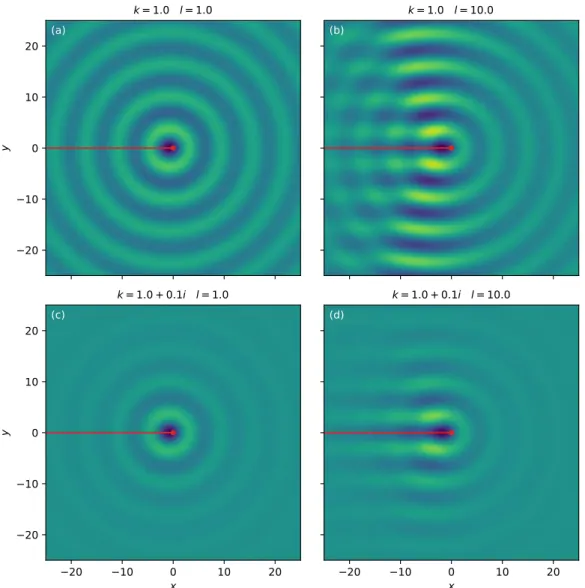
Figure 1. Wake generated by a point-particle traveling at constant velocity in a Helmholtz field with memory. Colormap show real part of h, after (6) and (8). Particle (red dot) is at
x = 0, y = 0. Red line shows trajectory.
where we have introduced the wake length l = uτ. For a change, we now write the solution to (1) in terms of the Hankel function of the first kind and of zeroth order, H0(1):
hs(x) = − i 4H
(1)
0 (kkxk). (8)
This is but a special version of (4), since the Hankel function is H0(1)= J0+ iY0. At this point,
its introduction is just a matter of convenience: this formulation allows us to separate the contributions of J0and of Y0by taking the real or imaginary part of h. We will examine the
implications of this choice, in terms of wave propagation and boundary conditions, in Section 4. We do not know of any analytical solution to (7) and (8). To approximate such solutions numerically, we first turn (7) into a path integral using a Laplace transform, and discretize it into a sum over a finite number of the particle’s past positions (Figure 1). When the particle travels
Figure 2. Cross-section of the wake generated by a point-particle traveling at constant velocity. Real and imaginary part of h after (6) and (8), for k = 1 and l = 10. Red line indicates particle trajectory (vertical position is arbitrary). This plot is a cross-section of Figure 1(b).
at moderate velocity (l = 1, Figure 1(a)), the wave field it produces is almost radially symmetric, like the Bessel function it originates from. A faster particle, however, generates the signature interference pattern of walking droplets, with its distinct crisscross behind the particle (l = 10, Figure 1(b)). This, of course, was to be expected, as a result of the present model’s lineage.
In the bouncing droplet experiments, the memory time is set by the decay rate of the Faraday wave. That the latter decays at all results from viscous dissipation, which also shortens the distance over which the Faraday wave can be excited. For consistency’s sake, any realistic model of bouncing droplet should relate the propagation radius of the Faraday wave to its memory [9]. Here, they appear as independent parameters, the former through the imaginary part of the wavenumber k, and the latter throughτ. If, leaving behind any attempt to realism, we keep l constant and add a finite imaginary part to k, we find that, away from the particle, the wave field dwindles (Figures 1(c) and (d)). Dissipation thus fits naturally into the present model, although it remains detached from the field’s memory.
The wave field of Figure 1 seems smooth, and a cross-section along the particle’s trajectory confirms this impression (Figure 2). The steady solution to the Helmholtz equation, though, is singular: the imaginary part of H0(1)diverges logarithmically at the origin:
H0(1)(z) ∼ 1 +2i
πlog(z), (9)
but this logarithmic divergence is smoothed out by the path integral of (6), which makes h a continuous function of space (Figure 2). This, however, does not apply to its gradient, which diverges near the particle. Since it is the latter that drives the particle’s motion, we will need special care to evaluate the force the wave field exerts upon a singular particle.
2.3. Motion of the particle
The endless variety of the bouncing droplets’ dynamics arises from their ability to interact with the wave field they generate. Having introduced the field with (1), and its memory with (5), we now need to specify how it acts upon the particle. Here again, we use the bouncing droplet as an inspiration, and simplicity as a guide. Accordingly, (i) the particle should move along the wave field’s gradient, (ii) the mathematical expression of the wave-induced force should apply
to a finite-size particle as well as to a singular one, and (iii) its evaluation should be numerically convenient.
The above requirements leave much room for interpretation. This arbitrariness notwithstand-ing, we propose that the particle moves according to:
˙xp= Re · α Ï ρ ∇h ¸ (10) whereα is a complex coupling factor of norm unity (αα = 1), and the overline denotes complex conjugation. As visible in the above expression, we consider an overdamped particle, the velocity of which is proportional to the force acting upon it. In other words, we consider only the zero-inertia limit of the particle’s horizontal dynamics [32]. A natural extension of this model would be to replace (10) with a momentum balance, but we leave it for future work.
To justify the form of (10), let us imagine a ball bobbing at the surface of a pool. Its vertical motion generates water waves, which in turn propel the ball across the water surface. The horizontal force the waves exert on the ball is proportional to the product of the gradient of the water surface with the ball’s draft [14]. Both quantities oscillate at the same frequency, and the only terms in this product that do not vanish on average combine into the scalar product of their complex amplitude—that is, Equation (10) (Appendix A). A classical, charged particle oscillating in its own electromagnetic field would we subjected to a force with a similar expression.
Returning to bouncing droplets, it is not obvious what the phase of the wave is when the droplet hits the bath’s surface, and receives a horizontal kick [9]. The argument ofα encodes for this unknown phase (its absolute value does not matter, as it can be absorbed into a new time scale). This parameter is obviously crucial: changing its sign, for instance, reverses the particle’s velocity. In some experiments, the phase of a bouncing droplet can change, thus turning this parameter into a new degree of freedom [19, 31]. Hereafter, we keep it constant.
Mathematically, the integral in (10) extends over the entire domain of the wave field. In fact, the support ofρ bounds the contribution of ∇h to the particle’s extension (Table 1). When the particle is small enough, Equation (10) amounts to the gradient of the wave amplitude at xp. Although we wrote our model with a finite-size particle in mind, hence the integral in (10), we expect no significant difference between this equation and its local, non-integral counterpart, at least when the particle is small enough (Re(k)rp ¿ 1) and the field continuous. These two conditions, however, seem to exclude each other; we will return to this issue in Section 3.
We are now equipped with a complete model for a particle in a Helmholtz field with memory, embodied by (1), (5) and (10). We have not checked yet whether this model remains consistent for an infinitesimal particle, but we prefer to postpone this mathematical endeavor until after a numerical interlude.
2.4. Numerical simulation
In some cases (point particle, simple boundaries), the Helmholtz equation may be solved ana-lytically [33]. The wave field h and the particle’s motion can then be computed at low numerical cost, a real advantage when long time series are required [6]. Here, we follow a different course, and use finite elements to approximate the wave field. This method uses more resources, but straightforwardly accommodates complicated boundaries, shallow barriers and finite-size parti-cles.
To solve the field equations (1) and (5) numerically, we write an implicit scheme for the discrete time evolution, and use FreeFem++ to mesh the domain and compute the finite element matrices [34] (Appendix B). For a fixed particle, this implicit scheme inherits the linearity of the original equations, but the motion of the particle, written implicitly, would induce a non-linearity.
To bypass this issue, we make the source term explicit by using the particle’s past position at each time step. The resulting semi-implicit scheme leaves much room for improvement, but its simplicity makes its implementation straightforward, and its implicit element ensures stability.
At this point, we need to choose boundary conditions for the wave field. Neumann and Dirichlet conditions are usual suspects, but we find that both tend to attract the particle towards the boundaries, thus ending the simulation (Gilet [33] found that the Neumann condition repels their point particle). Another option is to let the waves exit the domain with as little perturbation as possible, to approximate an infinite domain—this is what we do in Section 3.2. Here, we would like to confine the particle in a “corral” bounded by a repulsive boundary, like in the experiments of Harris et al. [20] and Sáenz et al. [35]. By trial and error, we found that a special, mixed boundary condition could do just that. Namely, requiring
n · ∇hs= βαhs (11)
along the boundary, whereβ is a real number of order one (typically, β = 5), ensures that the particle bounces off it, and remains in the field’s domain. In reality, when a bouncing droplet nears a wall, the wave-induced flow in the vibrated bath cannot be reduced to the horizontal dimensions any more. A fair representation of the bath’s boundaries requires a more sophisticated, three-dimensional model [36]; here again, at the cost of accuracy, we choose the simplicity of (11).
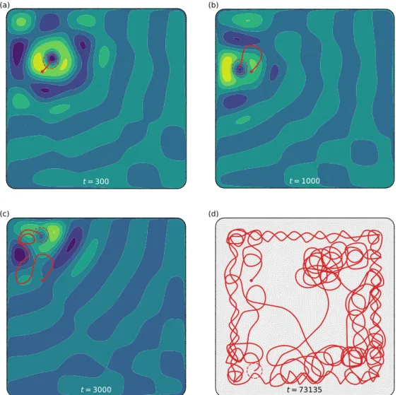
Figure 3 shows a particle wandering in a square box, according to numerical simulations of the present model. Initially, the particle stands near the upper left corner. A wave then builds up around it, and extends over the entire box, although its amplitude decreases away from the particle. In this asymmetric configuration, the wave sets the particle in motion. As the wave evolves around the moving particle, the latter departs from its initial direction, and draws a curved trajectory. The travel thus initiated will not stop before we end the simulation.
After a few tens of memory time (here,τ = 103), the particle has explored the box’s bound-aries, and sometimes ventured towards its center, with the wiggly gait of a walking droplet [20]. The convoluted shape of its trajectory (Figure 3(d)) evokes the chaotic paths of many experi-ments [37]. We have not evaluated how chaotic our system actually is, but its kinship with pre-vious models that proved so makes it likely that it is [33]. Finally, a favorably inclined eye might discern, in Figure 3(d), a coherent structure emerging from the apparent chaos of the trajectory, with locations more likely to be occupied than others [20, 23, 35].
A sound investigation of the disorder generated by the present model, and of the statistics emerging from it, would require long simulations and a reliable numerical scheme. Here, we assign ourselves a more modest goal: to locate self-propelled particles in the parameter space, and check that their velocity agrees with our numerical simulations.
3. Walkers
Following Protière et al. [2], we call “walker” a particle that propels itself by means of its own wave or, more accurately, the association of the particle and its wave, when both travel at the same velocity. The simulations of Section 2.4 are an indication that such walkers exist in our simplified model. In this section, we investigate ideal ones—those who travel alone, at constant velocity, in an infinite domain.
3.1. The walker’s equation
We now consider a particle that travels along the x axis at constant velocity u, while (1) and (6) set the surrounding wave field (Figure 1). For this system to make up a walker, the wave field must
Figure 3. Walker roaming across a Helmholtz field with memory. Finite-element simula-tion of (1), (5) and (10), with boundary condisimula-tion (11). Colormap shows real part of h (arbi-trary units). Red line: particle trajectory. Red dashed circle: particle’s support. Particle has a parabolic profile. Red dot indicates starting point. (Table 1). Parameters for this simula-tion are: k = exp(0.03iπ), rp= 0.4π/Re(k),τ = 103andα = exp(−iπ/4). (d) Final trajectory superimposed over finite-element mesh.
be such that the particle’s velocity satisfy (10) as well. This, we may guess, will only be possible for specific values of the model’s parameters, which we now look for.
If we are to exhibit simple analytical walkers, we need to assume that the particle is infinitesi-mal (ρ = δ), which allows us to express the wave field in terms of Bessel functions. We still need to decide which Bessel functions, that is, to prescribe a boundary condition at infinity. We chose to write the source wave field, hs, as a Hankel function of the first kind (Equation (8)). This choice means that a wave of complex amplitude hsand of positive pulsation propagates away from the particle (not towards the particle, as it would with a Hankel function of the second kind). We will come back to this point in Section 4.
We momentarily set aside the wave’s propagation and note that, for specific values of its parameters, the present model boils down to earlier ones, in which a smooth standing wave
drives the droplet [8]. For that,α only needs to be a pure imaginary number (α = ±i), and k a real one; then, only the imaginary part of h matters in (10), and only J0in (8). As visible in (9), the
former condition also rids us of the singularity of hs.
Motivated by this reasoning, we now assume thatα = ±i, until Section 3.3. We may then rewrite (10) for a point particle, and combine it with (7):
u = Re · α∂h ∂x ¸ x=0= Re hα l (h − hs) i x=0. (12)
As expected, this expression would be singular if the real part ofα did not vanish. Provided it does, we may replace hswith the Hankel function (Equation (8)), and h with the solution of (7). We find: u = ±1 4l · 1 lRe µZ ∞ 0 e−x/lH0(1)(kx) dx ¶ − 1 +π2arg(k) ¸ (13) where we recognize, in the form of the path integral, the Laplace transform of the Hankel function—a tabulated expression [38]. Remembering that l = uτ, we finally get the equation that implicitly defines the walker’s velocity:
τu2 = ± ( Re " µ 1 4− i 2πarcsinh µ 1 kuτ ¶¶ 1 p 1 + (kuτ)2 # −1 4+ 1 2πarg(k) ) , (14)
where the sign of the right-hand side is that of the imaginary part ofα.
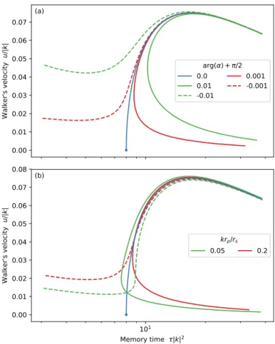
We could not find any analytical solution to (14), other than an immobile particle (u = 0). It is, however, straightforward to plot the locus of its solutions in the memory-velocity plane (Figure 4(a)). When the wavenumber is real (arg(k) = 0) and α = −i, the existence of walkers is conditional. Below a critical memory time ofτc= 8/|k|2, there cannot be any. At the critical memory time, the curve that represents (14) bifurcates, and the particle can walk at constant velocity. This velocity initially increases with the memory time, until it reaches a maximum at aboutτm≈ 16.9/|k|2, after which it slowly decays. As it does so, however, the length of its track in the wave field, l , keeps increasing (Figure 4(b)).
The sudden appearance of walkers above a critical value of the memory time is a familiar ob-servation in bouncing droplets experiments [2], which Oza et al. [32] interpret as a pitchfork bifur-cation. In accordance with this interpretation, we find that, when the memory time approaches its critical value (τ → 8/k2) while k remains real, the walker’s equation (14) reduces to
u k ∼ ±
p
2(k2τ − 8)
16p3 . (15)
Although consistent with a supercritical pitchfork bifurcation, this expression can only be part of the story, since the walker’s stability is beyond the reach of (14).
That the walker’s velocity decreases for large values of the memory time is more surprising, al-though Moláˇcek and Bush [19] report a slight drop of the velocity for some of their walkers. Exper-imentally, this regime (large values ofτ/|k|2) belongs to virtually uncharted territory, because it requires that the bath’s acceleration be exquisitely close to the Faraday threshold, without cross-ing it.
We now introduce some dissipation in the wave field, by letting the imaginary part of k depart from zero (arg(k) > 0, otherwise dissipation would inject energy in the wave field). Equation (14) is still valid, but its representation in Figure 4(a) changes radically: walkers can now exist for any value of the memory time. Their minute velocity, however, tempers this mathematical result— such slow walkers would be easily missed in an experiment. Even so, they should not be able to elude numerical simulations, to which we turn in the next section.
Figure 4. Walker’s equation for an infinitesimal particle, with coupling coefficient α = −i. (a) Particle’s velocity according to (14). Squares show numerical simulations (Section 3.2). (b) Memory length corresponding to the same equation.
3.2. Numerical stadium
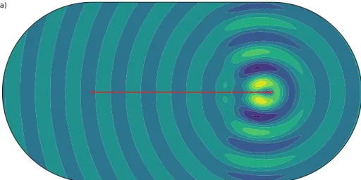
To evaluate our finite element simulation, we would like to compare the velocity of numerical walkers with (14). In a stadium-shaped domain, we introduce a small particle (rp= 0.1π/Re(k)), which we push forward at constant velocity until t = 10 (Figure 5(a)). We then let the particle relax to the walking mode, which it does after oscillating for some time around its final, steady velocity (Figure 5(b)). Oscillations like these occur in bouncing-droplet experiments too [39], where they sometimes last indefinitely [40].
Boundary conditions are crucial to this numerical experiment. The stadium’s wall should be invisible to the particle if it is to mimic the infinite domain that surrounds ideal walkers (Section 3.1). To make this boundary as transparent as possible, we choose a mixed boundary condition such that a wave coming exactly from the particle’s center would cross it without reflection. Mathematically,
n · ∇h = ik n · s (16)
where s is the unit vector pointing from the particle’s center towards the point of interest along the boundary. This unit vector varies along the boundary, and as the particle moves. At the cost of this inconvenience, the wave pattern around a numerical walker (Figure 5(a)) resemble its analytical counterpart (Figure 1).
Figure 5. Numerical simulation of a walker. Parameters are: memory time τ = 50, wavenumber k = exp(0.01iπ), coupling factor:α = −i). (a) Walker trajectory (red line) and real part of the Helmholtz field h at the end of the simulation (color map). Red dashed cir-cle shows actual size of particir-cle rp. Red dot indicates starting point. (b) Evolution of the walker’s velocity (blue line). Walker’s velocity is forced over shaded area. Green solid line: equilibrium velocity. Green dashed line: standard deviation of the walker’s velocity.
Once the particle has reached its cruising velocity, we measure the average value of the latter, and the associated uncertainty (Figure 5(b)). We then report these numerical observations on Figure 4(a), and find good agreement with (14). At this point, however, we ought to reveal a numerical trick we found to be necessary: we bound the particle to the x axis, lest it wiggle and drift sideways. That we needed to do so indicates an instability; we suggest it might be related to the self-orbiting modes of Labousse et al. [27], but we would need dedicated simulations to support this hypothesis. These, however, must be postponed and, for the sake of the present paper’s completeness, we now investigate the influence of the particle’s shape on walkers.
3.3. Particle shape
The shape of the particle, embodied by the distributionρ, affects the response of the wave field, and therefore the force it exerts on the particle. Based on this general argument, we expect the
velocity of a walker to depend on the particle’s shape. This point gets ambiguous, though, as the particle’s size vanishes, that is, whenρ approaches the Dirac distribution—and indeed, when α is imaginary, the velocity of an infinitesimal walker tells nothing about the particle’s shape and size (Section 3.1).
We now free the coupling factor from the requirements of Section 3.1: hereafter, the real part ofα may be finite. After (9) and (10), this component combines with the logarithmic singularity of the Hankel function and, as a result, the size of the particle should appear in the walker’s equation.
Let us consider a particle of finite size rp, much smaller than the field’s wavelength: Re(k)rp¿ 1. Combining (10) and (7), we find that we need to calculate two integrals to get the particle’s velocity: u = Re ·α l µÏ ρh − Ï ρhs ¶¸ . (17)
The first integral remains finite as the particle’s size tends to zero, and we thus approximate it with its value for a point particle (Section 3.1):
Ï ρh ≈ µ −i 4+ 1 2πarcsinh µ 1 kl ¶¶ 1 p 1 + (kl )2. (18)
So far, the particle’s size does not matter. The second integral of (17), however, diverges as the particle’s size vanishes—we need to refine the analysis one step further. The Helmholtz equation being linear, we may decompose the wave field hsas a sum of Green’s functions, weighted with the particle’s distributionρ. In line with Section 2.1, we assign the role of Green function to the Hankel function of (8), and write
hs(x) = − i 4 Ï x0H (1) 0 (x − x0)ρ(x0). (19)
The second integral of (17) then reads Ï ρ hs= − i 4 Ï x Ï x0ρ(x)H (1) 0 (x − x0)ρ(x0), (20)
an expression that depends on the particle’s distribution only. Considering a radially symmetric particle (Equation (2)), and using (9), we may rewrite (20) as
Ï ρ hs≈ − i 4+ 1 2πlog µ krp rs ¶ (21) where we have introduced the shape radius of the particle, rs, as
log rs= − Ï x Ï x0f (x) f (x 0) log kx − x0k. (22)
Hereafter, we name “shape factor” the logarithm of the shape radius (log rs). This quantity is defined for any well-behaved function f , and can sometimes be calculated analytically (Table 1 and Appendix C). Finally, we get a new expression for the walker’s equation, valid for any argument of the coupling factor:
τu2 = −Re( α2π " µ iπ 2 + arcsinh µ 1 kuτ ¶¶ 1 p 1 + (kuτ)2+ log µ −ikrrp s ¶#) . (23)
As expected, when the coupling factor α is a pure imaginary number, this expression be-comes (14) again; then, neither rpnor rsmatters. Otherwise, the walker’s velocity bears the sig-nature of the particle’s size and shape, through the ratio rp/rs. Even when the argument of the coupling factor is nearly −π/2 (α is almost −i), the walker’s equation changes qualitatively (Fig-ure 6(a)). When this argument is larger than −π/2, and the memory time is larger than a critical value, there are two solutions to the walker’s equation, each with its own velocity. Wind-Willassen
Figure 6. Walker’s equation for a small particle with real wavenumber (k = 1), according to (23). (a) Influence of the coupling parameter α, for the same particle (rp/rs = 1). (b) Influence of the particle’s shape and size, for the same coupling parameter. Solid lines: argα =π/2 + 0.001; dashed lines: argα =π/2 − 0.001. Solid blue line is that of (a).
et al. [40] first reported the coexistence of two walking modes with different velocities, but these
walkers also had distinct vertical dynamics—unlike the walkers of Figure 6(a). In tune with the present model, however, Bacot et al. [39] found that two modes could coexist while remaining synchronized with the bath’s oscillation.
Whenα < −π/2, there exist a single solution for any value of the memory time. As the latter approaches zero, the walker’s velocity diverges. Although unrealistic for bouncing droplets, this behavior makes sense in the present theoretical framework: as the field’s memory gets shorter,
h approaches hs, and the particle gets closer to the singularity, which propels it ever more powerfully.
Finally, we now fix the coupling factor, and vary the particle’s shape, that is, rp/rs(Figure 6(b)). We find that the walker’s curves, forα < −π/2 andα > −π/2, cross each other when the particle is small enough (rp/rs< 1), while they do not for larger ones—like in Figure 6(a). As the coefficient
rp/rsvaries, their intersection appears to draw the walker’s curve forα = −π/2.
Among the exotic walkers engendered by (23), some could well be unstable, and thus mostly irrelevant. Investigating their status, however, would bring us far beyond the scope of the present paper, which is only to devise a generic model inspired from the bouncing droplets. The features we could not stay away from—field dissipation (k), coupling factor (α) and particle’s
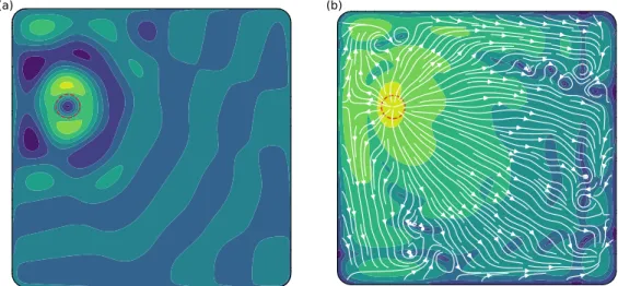
Figure 7. Energy flux and dissipation in a Helmholtz wave field, after (25). (a) Colormap shows real part of hs (arbitrary units). Red dashed circle: particle’s support. Parameters for this simulation are those of Figure 3. (b) Colormap shows the logarithm of dissipation, log(hshs). White lines with arrows show flux of energy, Im(hs∇hs).
details (rp/rs)—have already created a whole zoology of walkers. In the next section, instead of examining any of them in detail, we assess the extent of the jungle they dwell in.
4. Wave propagation and energy
So far, we have sidestepped the issue of wave propagation. In bouncing droplets models, one often assumes that the Faraday wave, sustained by the vertical oscillation of the bath, is standing—as opposed to propagative [2]. Although there are some standing-wave solutions to the Helmholtz equation, such as J0, most of its solutions propagate. In this section, we finally
consider this point.
4.1. Energy balance
Waves often transport energy, the flux of which relates to their propagation. The Helmholtz equation, which results from the separation of the wave field into a product of time- and space-dependent functions, transposes this relationship into a balance equation. Multiplying (1) with
hs, integrating over an arbitrary domain, and using Green’s theorem, we find: − Ï ∇hs· ∇hs+ I hsn · ∇hs+ k2 Ï hshs= Ï hsρ, (24)
of which we take the imaginary part: I n · Im(hs∇hs) + Im(k2) Ï hshs= Ï Im(hsρ). (25)
We identify, from left to right in the above equation, the energy flux, dissipation in the bulk and, on the right-hand side, the source term that represents the vibrating particle. Figure 7 shows this balance at work on a numerical example. The particle emits energy, which radiates about itself to finally dissipate in the domain’s bulk. Some energy also flows into the domain through the boundaries, due to the boundary condition (11). In a bold attempt at connecting the latter observation to experiments, we could relate it to surface tension, that would cause the bath’s
edge to respond more vigorously to vibrations than its bulk. Our numerical simulations suggest that this is how a simple boundary can repel bouncing droplets (a shallow layer can also be repellent [5]).
A somewhat dissatisfying issue with the present model is that the relaxation of h, which encodes the system’s memory, is disconnected from energy dissipation, as we pointed out in Section 2.2. In mathematical terms, Equation (5) cannot account for the energy that (25) is the balance of. To solve this issue, we would need to change how time alters the field h. We leave this matter for future work and, this issue notwithstanding, we now turn to the propagation of the Helmholtz wave associated with hs—and forget momentarily about h.
4.2. Standing wave
If hsis to be the complex amplitude of a standing wave, the corresponding wave field must be separable into a product of two real-valued functions, the first one depending on time, and the other on space. Mathematically,
Re[hs(x) exp(iωt)] = ˜hs(x) cos(ωt + ϕ), (26)
where ˜hs is a real-valued function, andϕ is a real constant. Taking the gradient of the above equation, we find that hs and ∇hsmust share the same phaseϕ everywhere. We may write this requirement as
Im(hs∇hs) = 0, (27)
where, after (25), we identify the energy flux. In words, a Helmholtz wave is standing when it transports no energy—an equivalence that accords with the intuitive notion of wave propagation. Equipped with the above definition, we readily see that the Helmholtz field of Figure 7 transports energy, and therefore corresponds to a propagating wave. In this simulation, the values of all the parameters are those of the walker of Figure 3; we must therefore acknowledge that this walker emits a propagating wave too. In fact, even the Hankel function H0(1), which we chose as our analytical reference, propagates energy—just like most solutions of (1), which need to transport energy away from the localized source.
Interference crisscross behind a moving particle (Figure 1), appearance of walkers beyond a critical memory time (Figure 4), chaotic-looking trajectory in a corral (Figure 3): all these phenomena, visually reminiscent of bouncing droplet experiments, occurred naturally in the present model. Yet, if shown in movies with a frame rate higher than the oscillation frequency, they would not look like the corresponding experiments at all: a wave would propagate away from the particle, in contrast with the Faraday wave that guides the droplets in reality. In fact, we would not know how to force a wave to be standing in the present model.
At this point, it is for the reader to judge how much of a drawback this is. Before they pronounce their verdict, however, we note that the numerical observations presented here, although preliminary, show that at least part of the strange behavior one observes on a vibrated bath of silicon oil extends to particles coupled with propagative waves—a broad class of systems indeed.
5. Discussion
The bouncing droplet of Couder et al. [1] has inspired a variety of theoretical models that couple a source particle to the wave it generates; the present paper offers but another one. Its advantages over its predecessor are few, but at least it reproduces the basic features of this system—walkers, interaction with boundaries, and memory.
The gist of bouncing droplet experiments is to challenge the exclusivity of quantum physics by producing fully-deterministic, macroscopic analogs. The present model suggests that such analogs do not even need any mathematical idiosyncrasy: homespun partial differential equa-tions will do. The familiarity of the latter opens the classical toolbox of Green’s funcequa-tions and the-orem, which unflinchingly expose the weakness of our model (its incomplete energy balance). The same tools, however, also expand the scope of the present theory to propagative waves, thus freeing the particle-wave couple from the Faraday instability, if only in theory.
To say this, though, is to open another box—Pandora’s. It is the curse of theory detached from experiments that it can create its own object matter; a tantalizing variation of the present model, for instance, is to replace (1) and (5) with a variant of the Shrödinger equation, of which the particle would be a source, as suggested by Andersen et al. [24]:
i∂h
∂t + ∇
2h + k2h = ρ. (28)
The resulting system, naturally possessed of a closed energy balance, is readily accessible to numerical simulations. In the present volume, Dagan and Bush [41] investigate another option: the Klein–Gordon equation—also conservative. Choosing the right system to investigate is a delicate decision but, in any case, it appears that the bouncing droplet can take off from its oil bath.
So, in the end, is any of this quantum mechanics? Probably not, although quantum analogs have drastically reduced the number of exclusively quantum phenomena. Fluid mechanics, then? In part, but the arrival of dry analogs [42] and numerical models [43] challenges this definition as well. Maybe, as Yves Couder used to say, “C’est de la physique.”
Acknowledgements
None of this work would have existed without inspiring discussions with Y. Couder and E. Fort, nor without their kind encouragement. The insightful remarks and poised skepticism of A. P. Petroff and P. Szymczak helped us tremendously. We are grateful to A. Lazarus, S. Protière, S. Perrard, M. Labousse, D. H. Rothman, F. Métivier, J. Neufeld, M. T. Biamonte, A. Abramian and A. Guérin for many illuminating and stimulating discussions.
Appendix A. Average force on a vibrating particle
Following Longuet-Higgins [14], let us consider a solid, compact object vibrating vertically at pulsationω in a horizontal wave field, possibly excited by the object itself, and that oscillates at the same frequency. We represent the object by its spatial distribution A(x, t ), and the field by
H (x, t )—two functions of space and time. Using complex notations, A(x, t ) = Re¡
ρ(x)eiωt¢
and H (x, t ) = Re¡h(x)eiωt¢ . (29) If we further assume that the horizontal force f(t ) acting on the particle is the integral of the field’s gradient over the object. It then reads
f(t ) = − Ï A∇H = −1 4 Ï ¡ ρeiωt + ρe−iωt¢ ³
∇heiωt+ ∇he−iωt ´
. (30)
Neglecting oscillating terms to keep only those that count on average, we finally write the average force 〈f〉 as 〈f〉 = −1 2Re Ï ρ∇h, (31) of which (10) is an instance.
Appendix B. Numerical scheme
We want to solve (1), (5) and (10) numerically. Integrating the second equation between two discrete times tnand tn+1, where n is the discretization index, we get
τ(hn+1− hn) +δt
2 (hn+1+ hn) =
δt
2 (hs,n+1+ hs,n) (32)
whereδt is the (constant) time step. This expression is implicit with respect to hnand hs,n, as a result of approximating time integrals with the trapezoidal rule. Treating (1) similarly but for the source term, we get
∇2(hs,n+1+ hs,n) + k2(hs,n+1+ hs,n) = 2ρn (33)
where we deliberately keep an explicit expression of the source term to avoid the non-linearity that a fully implicit scheme would yield. Having already lost much precision with this choice, we may write the last equation in a fully explicit form:
xp,n+1− xp,n= δt Re
·
αÏ ρn∇hn ¸
. (34)
To an expert eye, the above scheme will undoubtedly seem crude, but it proved tolerably efficient as a first shot.
Appendix C. Shape factor
Near the particle, Equation (1) resembles the Poisson equation—hence the logarithmic singular-ity in (22). We now rewrite the shape factor of (22) based on this observation. Let us define the Poisson field hP around the particle:
∇2hP= f , (35)
and require that, at infinity,
hP∼ 1
2πlog kxk. (36)
In two dimensions, the Green’s function of the Laplace equation is the logarithm, and we may thus express hP as the following integral:
hP(x) = 1 2π Ï x0 f (x0) log kx − x0k (37)
which we readily substitute into the definition of the shape factor, Equation (22): log rs= −2π
Ï
f hP. (38)
This definition is often more practical than (22). In particular, Equation (38) can be further simplified for compact, radially-symmetric distributions. Indeed, using Green’s theorem once again, we find log rs= 2π Ï r <1∇hP· ∇hP− 2 π Z r =1 hPn · ∇hP. (39)
Outside the support (r > 1), the distribution f vanishes. Since hPis radially symmetric, boundary condition (36) requires that
hP(r ) = 1
2πlog r for r > 1 (40)
and, by continuity, hPvanishes on the support’s boundary. Equation (39) thus becomes log rs= 4π2 Z1 0 r ¯ ¯ ¯ ¯ ∂hP ∂r ¯ ¯ ¯ ¯ 2 dr, (41)
obviously a positive quantity. This integral can often be evaluated analytically, based on the definition of hP (Equation (35)): ∂hP ∂r = 1 r Zr 0 r0f (r0) dr0. (42) Table 1 gathers the results of this procedure for a few exemplary distributions.
Appendix D. Gaussian particle
We wish to calculate the shape factor of a particle with a Gaussian distribution:
f (r ) =e
−r2
π . (43)
We first calculate the Poisson field of which this distribution is a source, based on (35) and (36):
hP(r ) = 1 2π · log r +E1(r 2) 2 ¸ (44) where E1is the exponential integral. Combining this result with (38), we finally get
log rs= − Z∞
0 [2 log r + E1
(r2)]r e−r2dr =1
2(γ − log2) ≈ −0.058 (45) whereγ is the Euler–Mascheroni constant.
References
[1] Y. Couder, S. Protiere, E. Fort, A. Boudaoud, “Dynamical phenomena: walking and orbiting droplets”, Nature 437 (2005), no. 7056, p. 208.
[2] S. Protière, A. Boudaoud, Y. Couder, “Particle–wave association on a fluid interface”, J. Fluid Mech. 554 (2006), p. 85-108.
[3] J. W. M. Bush, Y. Couder, T. Gilet, P. A. Milewski, A. Nachbin, “Introduction to focus issue on hydrodynamic quantum analogs”, Chaos 28 (2018), no. 9, 096001.
[4] Y. Couder, E. Fort, “Single-particle diffraction and interference at a macroscopic scale”, Phys. Rev. Lett. 97 (2006), no. 15, 154101.
[5] A. Eddi, E. Fort, F. Moisy, Y. Couder, “Unpredictable tunneling of a classical wave-particle association”, Phys. Rev.
Lett. 102 (2009), 240401.
[6] S. Perrard, M. Labousse, M. Miskin, E. Fort, Y. Couder, “Self-organization into quantized eigenstates of a classical wave-driven particle”, Nat. Commun. 5 (2014), p. 3219.
[7] J. W. M. Bush, “Quantum mechanics writ large”, Proc. Natl Acad. Sci. USA 107 (2010), no. 41, p. 17455-17456. [8] E. Fort, A. Eddi, A. Boudaoud, J. Moukhtar, Y. Couder, “Path-memory induced quantization of classical orbits”, Proc.
Natl Acad. Sci. USA 107 (2010), no. 41, p. 17515-17520.
[9] P. A. Milewski, C. A. Galeano-Rios, A. Nachbin, J. W. M. Bush, “Faraday pilot-wave dynamics: modelling and computation”, J. Fluid Mech. 778 (2015), p. 361-388.
[10] M. Rabaud, Y. Couder, N. Gerard, “Dynamics and stability of anomalous Saffman–Taylor fingers”, Phys. Rev. A 37 (1988), no. 3, p. 935.
[11] E. Lajeunesse, Y. Couder, “On the tip-splitting instability of viscous fingers”, J. Fluid Mech. 419 (2000), p. 125-149. [12] Y. Couder, “Viscous fingering as an archetype for growth patterns”, Perspect. Fluid Dyn. 2 (2000), no. 4.2, p. 3. [13] D. Bohm, M. Weinstein, “The self-oscillations of a charged particle”, Phys. Rev. 74 (1948), no. 12, p. 1789.
[14] M. S. Longuet-Higgins, “The mean forces exerted by waves on floating or submerged bodies with applications to sand bars and wave power machines”, Proc. R. Soc. Lond. A 352 (1977), no. 1671, p. 463-480.
[15] P.-T. Brun, D. M. Harris, V. Prost, J. Quintela, J. W. M. Bush, “Shedding light on pilot-wave phenomena”, Phys. Rev.
Fluids 1 (2016), no. 5, 050510.
[16] D. M. Harris, J. Quintela, V. Prost, P.-T. Brun, J. W. M. Bush, “Visualization of hydrodynamic pilot-wave phenomena”,
J. Vis. 20 (2017), no. 1, p. 13-15.
[17] G. Pucci, D. M. Harris, L. M. Faria, J. W. M. Bush, “Walking droplets interacting with single and double slits”, J. Fluid
Mech. 835 (2018), p. 1136-1156.
[18] Y. Couder, E. Fort, C.-H. Gautier, A. Boudaoud, “From bouncing to floating: noncoalescence of drops on a fluid bath”,
[19] J. Moláˇcek, J. W. M. Bush, “Drops walking on a vibrating bath: towards a hydrodynamic pilot-wave theory”, J. Fluid
Mech. 727 (2013), p. 612-647.
[20] D. M. Harris, J. Moukhtar, E. Fort, Y. Couder, J. W. M. Bush, “Wavelike statistics from pilot-wave dynamics in a circular corral”, Phys. Rev. E 88 (2013), no. 1, 011001.
[21] J. Arbelaiz, A. U. Oza, J. W. M. Bush, “Promenading pairs of walking droplets: dynamics and stability”, Phys. Rev.
Fluids 3 (2018), no. 1, 013604.
[22] A. Eddi, A. Decelle, E. Fort, Y. Couder, “Archimedean lattices in the bound states of wave interacting particles”,
Europhys. Lett. 87 (2009), no. 5, 56002.
[23] J. W. M. Bush, “Pilot-wave hydrodynamics”, Annu. Rev. Fluid Mech. 47 (2015), p. 269-292.
[24] A. Andersen, J. Madsen, C. Reichelt, S. R. Ahl, B. Lautrup, C. Ellegaard, M. T. Levinsen, T. Bohr, “Double-slit experiment with single wave-driven particles and its relation to quantum mechanics”, Phys. Rev. E 92 (2015), no. 1, 013006.
[25] A. Eddi, E. Sultan, J. Moukhtar, E. Fort, M. Rossi, Y. Couder, “Information stored in faraday waves: the origin of a path memory”, J. Fluid Mech. 674 (2011), p. 433-463.
[26] M. Labousse, A. U. Oza, S. Perrard, J. W. M. Bush, “Pilot-wave dynamics in a harmonic potential: quantization and stability of circular orbits”, Phys. Rev. E 93 (2016), no. 3, 033122.
[27] M. Labousse, S. Perrard, Y. Couder, E. Fort, “Self-attraction into spinning eigenstates of a mobile wave source by its emission back-reaction”, Phys. Rev. E 94 (2016), no. 4, 042224.
[28] S. Perrard, M. Labousse, “Transition to chaos in wave memory dynamics in a harmonic well: deterministic and noise-driven behavior”, Chaos 28 (2018), no. 9, 096109.
[29] G. Pucci, P. J. Sáenz, L. M. Faria, J. W. M. Bush, “Non-specular reflection of walking droplets”, J. Fluid Mech. 804 (2016), R3.
[30] A. Nachbin, P. A. Milewski, J. W. M. Bush, “Tunneling with a hydrodynamic pilot-wave model”, Phys. Rev. Fluids 2 (2017), no. 3, 034801.
[31] M. M. P. Couchman, S. E. Turton, J. W. M. Bush, “Bouncing phase variations in pilot-wave hydrodynamics and the stability of droplet pairs”, J. Fluid Mech. 871 (2019), p. 212-243.
[32] A. U. Oza, R. R. Rosales, J. W. M. Bush, “A trajectory equation for walking droplets: hydrodynamic pilot-wave theory”,
J. Fluid Mech. 737 (2013), p. 552-570.
[33] T. Gilet, “Quantumlike statistics of deterministic wave-particle interactions in a circular cavity”, Phys. Rev. E 93 (2016), no. 4, 042202.
[34] F. Hecht, “New development in freefem++”, J. Numer. Math. 20 (2012), no. 3–4, p. 251-265.
[35] P. J. Sáenz, T. Cristea-Platon, J. W. M. Bush, “Statistical projection effects in a hydrodynamic pilot-wave system”, Nat.
Phys. 14 (2018), no. 3, p. 315-319.
[36] M. Durey, P. A. Milewski, Z. Wang, “Faraday pilot-wave dynamics in a circular corral”, J. Fluid Mech. 891 (2020), p. A3. [37] S. Perrard, M. Labousse, E. Fort, Y. Couder, “Chaos driven by interfering memory”, Phys. Rev. Lett. 113 (2014), no. 10,
104101.
[38] A. D. Polyanin, A. V. Manzhirov, Handbook of Integral Equations, CRC Press, 1998.
[39] V. Bacot, S. Perrard, M. Labousse, Y. Couder, E. Fort, “Multistable free states of an active particle from a coherent memory dynamics”, Phys. Rev. Lett. 122 (2019), no. 10, 104303.
[40] Ø. Wind-Willassen, J. Moláˇcek, D. M. Harris, J. W. M. Bush, “Exotic states of bouncing and walking droplets”, Phys.
Fluids 25 (2013), no. 8, 082002.
[41] Y. Dagan, J. W. M. Bush, “Hydrodynamic quantum field theory”, C. R. Méc. (2020) (This issue). [42] A. Halev, D. M. Harris, “Bouncing ball on a vibrating periodic surface”, Chaos 28 (2018), no. 9, 096103.
[43] S. E. Turton, M. M. P. Couchman, J. W. M. Bush, “A review of the theoretical modeling of walking droplets: toward a generalized pilot-wave framework”, Chaos 28 (2018), no. 9, 096111.