HAL Id: insu-03011315
https://hal-insu.archives-ouvertes.fr/insu-03011315
Submitted on 18 Nov 2020
HAL is a multi-disciplinary open access
archive for the deposit and dissemination of
sci-entific research documents, whether they are
pub-lished or not. The documents may come from
teaching and research institutions in France or
abroad, or from public or private research centers.
L’archive ouverte pluridisciplinaire HAL, est
destinée au dépôt et à la diffusion de documents
scientifiques de niveau recherche, publiés ou non,
émanant des établissements d’enseignement et de
recherche français ou étrangers, des laboratoires
publics ou privés.
Numerical simulations help revealing the dynamics
underneath the clouds of Jupiter
Johannes Wicht, Thomas Gastine
To cite this version:
Johannes Wicht, Thomas Gastine. Numerical simulations help revealing the dynamics underneath the
clouds of Jupiter. Nature Communications, Nature Publishing Group, 2020, 11 (1),
�10.1038/s41467-020-16680-0�. �insu-03011315�
Numerical simulations help revealing
the dynamics underneath the clouds
of Jupiter
Johannes Wicht
1✉
& Thomas Gastine
2Since its arrival at Jupiter in 2016, NASA
’s Juno spacecraft has been performing
high-precision measurement of the gravity and magnetic
fields. When combined
with numerical simulations, they provide a unique window to the dynamics in the
planet
’s deep atmosphere.
A very different atmosphere
Earth’s atmosphere adds only a mere 20 km to the mean 6371 km radius of our rocky home planet. We all experience the complicated dynamics of this thin envelope when trying to keep pace with the capricious weather. Meteorologists rely on a continuous stream of data and enormous computational efforts to model this dynamics and have learned that Earth’s irregular surface and the variable solar irradiation play key roles. This is very different on Jupiter. The king among planets is a gas giant that mainly consists of hydrogen and helium. A denser core of unknown composition only occupies a smaller central portion (Fig. 1b). Since the typical atmospheric pressure reaches one bar at Earth’s surface, scientist traditionally also refer to the one bar level at a mean radius of rJ= 69,911 km as the lower boundary of Jupiter’s atmosphere.
However, this is an arbitrary choice. Compared to the precious gas envelope around Earth, Jupiter’s hydrogen/helium envelope is virtually bottomless, and the solar radiation only pene-trates a tiny outer fraction. Not surprisingly, the dynamics is also very different.
Unfortunately, we can only observe Jupiter’s top layers directly1. The wandering of the colorful
clouds reveals a system of fast westward- and eastward-directed zonal jets that encircle the whole planet. The jets sculpture the planet’s beautiful stripes. The big red spot and numerous smaller spots, on the other hand, correlate with slower eddies. Earth-bound telescopes penetrate the thick cloud cover down to roughly 60 km below rJ. The Galileo probe2, which entered Jupiter in 1995, survived
to a depth of about 160 km. NASA’s Juno spacecraft3, currently in orbit around Jupiter, carries a
powerful microwave radiometer, which can penetrate to a depth of perhaps 500 km. This is still less than 1% of the planet’s radius. In order to peer deeper, we must resort to more indirect means and combine observations with theoretical and numerical studies of the planet’s interior dynamics.
Numerical simulations of jets and magneticfield
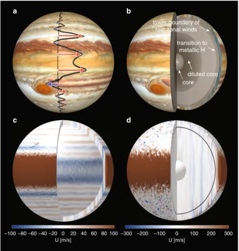
Studies of motions in deeper atmospheres that are driven by the cooling of the planet rather than by solar irradiation seem particularly relevant4–6. The respective results highlight the key role of the planetary rotation in structuring the turbulentflows. Three important jet properties become apparent: First, the jets naturally develop from the small-scale turbulence. Second, they form concentric cylinders that are aligned with the planetary rotation axis (Fig.1c). Third, the width of the jets depends on the depth of the modeled shell and is most realistic for a lower boundary at
1Max Planck Institute for Solar System Research, Göttingen, Germany.2Institut de Physique du Globe de Paris, Paris, France. ✉email:[email protected]
123456789
0.94 rJ5. Which physical effect could put on the brakes at this
specific depth? Perhaps the magnetic forces, which were neglected in these simulations?
Like Earth, Jupiter has a global magneticfield that is produced by a dynamo process. Earth’s dynamo operates in the liquid iron core, but what about Jupiter? Below about 0.9 rJ, the extreme
pressures squeeze the atoms so close together that hydrogen becomes metallic7. Above 0.9 r
J, the electrical conductivity
decreases rapidly in the so-called transition region and eventually becomes negligible. Since dynamo action and the magnetic Lor-entz forces scale with conductivity, they are most efficiently in the inner metallic region but can be significant in the transition region. Where the Lorentz forces remain negligible in the very-outer atmosphere, the jets should retain their cylindrical geo-metry. Somewhere in the transition region, however, the Lorentz forces would kick in abruptly and quench the jets over a depth range of about 1000 km8.
To test these ideas, scientists ran a number of ambitious numerical simulations that not only model the jets but also the
deeper dynamo processes. The results reveal interesting but also puzzling new aspects9–12. The magneticfield of Jupiter, like the field of Earth, is dominated by an axial dipole. However, the jets tend to promote magneticfield configurations with rather weak axial dipole contributions. The key to reproducing Jupiter’s magnetic field therefore lies in limiting the role of the jets in the dynamo process. Rather than simply quenching the jets in the transition region, however, the simulation choses another option (Fig. 1d): the Lor-entz forces push the eastward equatorial jet to the outer envelope but slow down rather than truncate the remaining jets10,11.
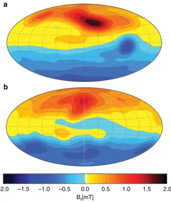
These simulations cannot exactly reproduce Jupiter’s complex jet structure (Fig.1d). They also use unrealistically high viscosities to suppress the smallest turbulent features that cannot be resolved with current computer resources. One consequence is that the zonal winds are not as dominant as on Jupiter. However, the models seem to capture the essence of the dynamo process and reproduce the very inhomogeneousfield distribution that sets the magneticfields of Jupiter and Earth apart13. Particularly obvious is the concentration of outward directedfield (Fig.2a, yellow and
a b
d c
lower boundary of fast zonal winds
transition to metallic H diluted core core –300 –200 –100 0 100 200 300 100 80 60 40 20 0 –20 –40 –60 –80 –100 U [m/s] U [m/s]
Fig. 1 The zonal winds and interior structure of Jupiter. a Jupiter’s cloud level zonal jets projected onto a Hubble surface image. The black line shows the jet velocity profile while red arrows indicate eastward and blue arrows westward jet maxima. The fastest jets are eastward and reach a maximum velocity of about 130 m/s.b Interior model with an outer region of fast zonal jets (5% in radius), the transition to the metallic hydrogen region (10% in radius), a core (20% in radius), and a possible region of denser material that may consist of diluted core material18.c Color contours of the azimuthalflow U in a snapshot of a simulation in a shell covering 10% in radius6. Red and blue colors indicate eastward and westward winds respectively.d Color contours of the azimuthalflow U in a snapshot of a Jupiter-like dynamo simulation10. The black circle separates the weakly conducting outer and highly conducting inner region. Lorentz forces confine the dominant prograde equatorial jet to the outer region and brake the other jets. On time average, only the equatorial jet persists. The other azimuthalflows are more time dependent and merge to form a broad slow westward flow. The image of Jupiter’s surface in panels (a) and (b) is courtesy to NASA and ESA. Credits go to A. Simon (Goddard Space Flight Center) and M.H. Wong (University of California, Berkeley). The simulations illustrated in panels (c) and (d) have been performed with the dimensionless computer code MagIC. The code calculates the azimuthalflows in units of a Rossby number: Ro= U/(rJΩ). This has been rescaled to m/s by assuming a mean radius of rJ= 6.9911 × 10⁶m and a planetary rotation rate of
Ω = 1.759 × 10⁻⁴s−1.
red) in a latitudinal band between 30 and 60° north. In the southern hemisphere, a prominent patch of inward (blue) field sits just south of the equator, but overall the field seems more homogeneous than in the north. The simulation snapshot (Fig. 2b) shows very similar banded structures in the northern hemisphere10. The southern blue patch is missing, but similar
features appear later in the simulation.
The numerical models generate the Jupiter-like magneticfield in a two-stage process. A deeper primary dynamo produces the main dipole-dominated magneticfield in the metallic region. A shallower secondary dynamo operates where the equatorial jet reaches sizeable conductivities in the transition region10,11and generates the banded
or patchy features observed at low to mid latitude. This suggests that the jets contribute to shaping the magneticfield of Jupiter. They also give rise to density difference and thus to tiny modifications of Jupiter’s gravity field. Both magnetic and gravity measurements can thus potentially constrain the deeper jet structure.
Exploiting gravity and magnetic data
For thefirst time, Juno gravity measurements are precise enough to detect the tiny signature of the deeper zonal jets. However, the interpretation is difficult. The first attempts in principle adopt the cylindrical jet geometry but report that an additional gradual decay with depth is required14,15: While the jets blow with up to
150 m/s at cloud level, they slow down to about 10 m/s at 0.96 rJ
and to 2 m/s at 0.94 rJ. This is at odds with the abrupt decay
expected from Lorentz forces. A comparison of the magnetic fields measured by Juno and by previous spacecrafts gives rise to further doubts: The modest variations over the 45-year time span covered by the missions indicate that the jet velocity cannot exceed 0.01 m/s at 0.94 rJ16. Further analysis of gravity and
magnetic data seem in order to resolve the contradictions.
A stable layer in the outer atmosphere of Jupiter?
A recent numerical study17of jets in a simplified Cartesian box puts a promising new idea on the table: An additional stable layer where the density stratification tend to suppresses radial motions. Lorentz forces drive radialflows in the transition region, which are much slower than the jets and therefore normally have little effect. However, once the radialflows penetrate a stable layer and encounter the density stratification, they can promote a very effectively quenching of the jets.
The upper boundary of the stable layer should lie between 0.94 rJand 0.96 rJ. Interestingly, some newer interior structure models
suggest a somewhat deeper stable layer below 0.93 rJ18.
How-ever, it remains unclear which physical mechanism could support such a layer. Helium rain, a process deemed responsible for a thick stable layer in Saturn, only happens in metallic hydrogen and thus not above 0.9 rJin Jupiter.
Conclusion
The combination of observations and numerical simulations provides a powerful tool for peering underneath the cloud deck of Jupiter. The results suggest that the fast jets are limited to the outer 4–6% in radius, assume a cylindrical geometry, and are abruptly quenched at the lower boundary, perhaps by a com-bination Lorentz forces and a stable layer. While first evalua-tions of Juno gravity data propose a more gradual quenching, the analysis is complex and ambiguous and leaves room for alternative models.
State-of-the-art numerical dynamo simulations reproduce many features of Jupiter’s magnetic field and highlight the important role of the dominant equatorial jet. However, they fail in reproducing the multiple jet system. Two options for improvement are the adoption of lower viscosities and the implementation of a stable layer. Juno gravity data also indicate a higher concentration of heavy elements below perhaps 0.6 rJ18.
Future numerical studies could clarify whether such a scenario is consistent with Jupiter’s magnetic field.
The simulations also suggest that Jupiter's magneticfield bears signs of zonal jet action. However, deducing the jet properties from the magnetic field structure is very challenging. Observa-tions of magnetic field variations, on the other hand, are an established tool for accessing the dynamic in Earth’s core and have already proven useful at Jupiter16. There is a chance that
Juno will observe minor variations during its mission time. More promising data will become available when ESA’s Juice spacecraft arrives at Jupiter in 2029.
Code availability
Most of the simulations discussed here were performed with the code MagIC, which is freely available at GitHub:https://github.com/magic-sph.
Received: 14 February 2020; Accepted: 18 May 2020;
References
1. Guillot, T. & Fletcher, L. N. Revealing giant planet interiors beneath the cloudy veil. Nat. Comm. 11, 1555 (2020).
2. Young, R. E., Smith, M. A. & Sobeck, C. K. Galileo probe: in situ observations of Jupiter’s atmosphere. Science 272, 837–838 (1996).
3. Bolton, S. J. et al. The Juno mission. Space Sci. Rev. 213, 5–37 (2017). 4. Lian, Y. & Showman, A. P. Generation of equatorial jets by large-scale latent
heating on the giant planets. Icarus 207, 373 (2010).
5. Gastine, T., Heimpel, M. & Wicht, J. Zonalflow scaling in rapidly-rotating compressible convection. Phys. Earth Planet. Int. 232, 36–50 (2014). 6. Heimpel, M., Gastine, T. & Wicht, J. Simulation of deep-seated zonal jets and
shallow vortices in gas giant atmospheres. Nat. Geosci. 9, 19–23 (2016).
–2.0 –1.5 –1.0 –0.5 0.0 0.5 1.0 1.5 2.0
Br[mT] a
b
Fig. 2 The magneticfield of Jupiter. a Jupiter's radial surface field model JRM09 based on Juno measurements3.b Snapshot of the radial surface field in a Jupiter-like dynamo simulations10. Outgoingfield is shown in yellow and red and ingoingfield in blue.
7. French, M. et al. Ab initio simulations for material properties along the Jupiter adiabat. APJ 202, 5 (2012).
8. Wicht, J., Gastine, T. & Duarte, L. D. V. Dynamo action in the steeply decaying conductivity region of Jupiter‐like dynamo models. J. Geophys. Res: Planets 124, 837–863 (2019).
9. Jones, C. A. A dynamo model of Jupiter’s magnetic field. Icarus 241, 148 (2014).
10. Gastine, T., Wicht, J., Duarte, L. D. V., Heimpel, M. & Becker, A. Explaining Jupiter’s magnetic field and equatorial jet dynamics. Geophys. Res. Lett. 41, 5410–5419 (2014).
11. Duarte, L. D. V., Wicht, J. & Gastine, T. Physical conditions for Jupiter-like dynamo models. Icarus 299, 206–221 (2018).
12. Dietrich, W. & Jones, C. A. Anelastic spherical dynamos with radially variable electrical conductivity. Icarus 305, 15–32 (2018).
13. Connerney, J. E. P. et al. A new model of Jupiter’s magnetic field from Juno’s first nine orbits. Geophys. Res. Lett. 45, 2590–2596 (2018).
14. Kaspi, Y. et al. Jupiter’s atmospheric jet streams extend thousands of kilometres deep. Nature 555, 223–226 (2018).
15. Kong, D., Zhang, K., Schubert, G. & Anderson, J. D. Origin of Jupiters cloud-level zonal winds remains a puzzle even after Juno. Proc. Natl Acad. Sci. USA 115, 8499–8504 (2018).
16. Moore, K. M. et al. Time variation of Jupiter’s internal magnetic field consistent with zonal wind advection. Nat. Astron. 3, 730–735 (2018). 17. Christensen, U. R., Wicht, J. & Dietrich, W. Mechanisms for limiting the
depth of zonal winds in the gas giant planets. ApJ 890, 61 (2020). 18. Debras, F. & Chabrier, G. New models of Jupiter in the context of Juno and
Galileo. ApJ 872, 100 (2019).
Acknowledgements
This work was supported by the DFG (German Science Foundation) within the Special Priority Program 1488 PlanetMag. Computations were carried out at the Max Planck Computing & Data Facility, which also helped with code development.
Author contributions
J.W. wrote most of the text. T.G. performed performed most of the numerical simula-tions discussed here. Both authors contributed to the development of the computer code MagIC and to the data analysis.
Competing interests
The authors declare no competing interests.
Additional information
Correspondence and requests for materials should be addressed to J.W.
Reprints and permission information is available athttp://www.nature.com/reprints Publisher’s note Springer Nature remains neutral with regard to jurisdictional claims in published maps and institutional affiliations.
Open Access This article is licensed under a Creative Commons Attribution 4.0 International License, which permits use, sharing, adaptation, distribution and reproduction in any medium or format, as long as you give appropriate credit to the original author(s) and the source, provide a link to the Creative Commons license, and indicate if changes were made. The images or other third party material in this article are included in the article’s Creative Commons license, unless indicated otherwise in a credit line to the material. If material is not included in the article’s Creative Commons license and your intended use is not permitted by statutory regulation or exceeds the permitted use, you will need to obtain permission directly from the copyright holder. To view a copy of this license, visithttp://creativecommons.org/ licenses/by/4.0/.
© The Author(s) 2020