Detection of DNA polymorphisms in thermal gradients via a scanning laser confocal system

K

₁

Detection of DNA Polymorphisms in Thermal Gradients

via a Scanning Laser Confocal System.

by

Matthew Ryan Graham

S.B. Physics

Massachusetts Institute of Technology, 1998

SUBMITTED TO THE DEPARTMENT OF MECHANICAL ENGINEERING IN

PARTIAL FULFILLMENT OF THE REQUIREMENTS FOR THE DEGREE OF

MASTER OF SCIENCE IN MECHANICAL ENGINEERING

AT THE

MASSACHUSETTS INSTITUTE OF TECHNOLOGY

JUNE 2000

D 2000 Massachusetts Institute of Technology.

All rights reserved.

Signature of Author:

Certified by:

, , \.

--Department of Mechanical Engineering

May

5,

2000

Ian W. Hunter

Professor of Mechanical Engineering and Professor of BioEngineering

_,,,,.hesis Supervisor

Accepted by:

Graduate Officer,

IM

LS1JE

I'S TITUTE

OFT

'ECI.NOLOGY

Ain A. Sonin

Professor of Mechanical Engineering

Department of Mechanical Engineering

MASSACHUSETTS INSTITUTE

OF

TECHNOLOGY

Detection of DNA Polymorphisms in Thermal Gradients

via a Scanning Laser Confocal System.

by

Matthew Ryan Graham

Submitted to the Department of Mechanical Engineering

on May

5,

2000 in Partial Fulfillment of the

Requirements for the Degree of Master of Science in

Mechanical Engineering

ABSTRACT

Discovery and detection of single nucleotide polymorphisms (SNPs) in DNA

has become an important topic of research in the past few years. However, SNPs are very

often detected by the labor intensive process of sequencing lengths of DNA A scanning

laser confocal capillary gel electrophoresis (CGE) system has been designed to provide a

faster and more efficient method of detecting SNPs in short lengths of DNA.

The velocities of migrating DNA segments were measured over 100 mm as

they moved through a specially designed CGE system. The velocity of these DNA

segments was found to have an exponential relationship to the segment length. Also, a

thermal gradient was then applied to the length of the capillary. As the DNA migrated, it

was heated, and as the segments denatured, the DNA bands slowed. A "GC clamp" kept

the two partially denatured strands from completely separating. When the thermal

gradient was applied to the capillaries, the DNA segments demonstrated a velocity shift.

However, the DNA did not show the expected sudden "break" in the velocity curve, but

rather a more complex melting/velocity curve.

Thesis Supervisor: Ian W. Hunter

Acknowledgments:

Thank you to everyone in the Bioinstrumentation Laboratory and in Professor

Lerman's Lab in the Biology Department. My time here would not have been nearly half

as fun without you. Special thanks to Professor Ian Hunter for giving me the chance to

learn so much in such an exciting environment. And most importantly, thank you to my

parents for always supporting me no matter where I've chosen to go.

Table of Contents

I. B a ck g ro u n d ...

5

A. DNA Structure...5

B. Single Nucleotide Polymorphisms...

5

II . T h e o ry ...

6

A. M otion of DNA in capillary...6

1. Electrophoresis...6

2. Electroosmotic Flow...

7

B. DNA and SNPs...

9

C. Confocal Optical Systems...

10

D . Temperature Gradient...

12

III. Experimental Design & Setup...14

A. Optical Subsystem ...

14

B. Capillary Plate and Heaters...

16

C. Capillary Interface...

17

D. Capillaries & Gel Chemistry...18

E. Electrical Subsystem...

21

F. Computer Automation and System Operation...22

G. System M ounting and Housing...

23

IV . R e su lts...2

4

A . S im p le R u n ...

2 4

B . S im p le S can ...

2 5

C . G rad ient S can ...

2 6

V . A n aly sis...2

8

A. DNA Velocities...28

B . D en atu rant...2

9

C. Curve Tracking and Identification...

30

V I. C o n clu sio n s...3

1

VII. References...32

Appendix A: M ATLAB@ Code...

34

Appendix B: Electrical Diagrams...36

Appendix C: M echanical Drawings...

38

Appendix D: Derivation of Electroosmotic Flow ...

40

I. Background

A. DNA Structure

The structure of DNA was discovered in 1953 by James Watson and Francis

Crick (Watson and Crick, 1953). DNA, which is an organic polymer that contains all of

the genetic code for life, consists, structurally, of the backbone and bases. The backbone

of DNA is further divided into alternating sugars and phosphate groups forming a linear

strand. Each unit of DNA can be segmented into a single sugar and phosphate group

along with a single base. These three components compose the structure known as a

nucleotide. The nucleotide is the base unit of information in DNA. Nucleotides are

differentiated by their bases, of which there are four types in DNA (there is a fifth one in

RNA). These bases are Adenine (A), Cytosine (C), Guanine (G), and Thymine (T).

Each single strand of DNA has a direction sense and can be represented by a

sequence of these four bases. Genomic DNA is typically found in double-stranded form

(dsDNA), in which two strands arrange themselves in a complementary, anti-parallel

sense. The bases are arranged in complementary base pairs (A with T, and C with G)

forming a series of hydrogen bonds between the two strands. The A-T bond consists of

two hydrogen bonds while the G-C is made up of three. These two strands usually form

into a secondary structure known as the double-helix, a form that most people now

recognize as pertaining to the workings inside their bodies.

B. Single Nucleotide Polymorphisms

Single nucleotide polymorphisms, or SNPs, are normal mutations in human

DNA which occur at a single base pair location. To qualify as SNPs, the least common of

these mutation combinations, or alleles, must occur at a rate of 1% or greater in the

population. In any SNP location, it is possible to have four different allele combinations:

A-T, T-A, G-C, and C-G. The direction sense of DNA makes the difference between the

G-C and C-G alleles (as well as between the A-T and T-A alleles) very important, and

they must be considered as separate cases. However, in human DNA, most SNPs occur

with only two different alleles, and SNPs with three or four are very rare (Brookes, 1999).

Certain SNPs are known to predispose people to certain diseases. In these

cases the relationship can be simple: persons with one SNP allele are more likely to have a

certain genetic disease than are those with the other allele. However, researchers are only

now beginning to investigate the vast relationships and interactions between multiple

SNPs and disease. This effort will require large public libraries of SNPs and

accompanying population information. Already, a few major efforts are under way to

establish such public libraries (dbSNP, HGBASE).

Detecting SNPs in a fast and cost effective way is an important challenge to be

met in this research. Currently, SNPs are detected by sequencing a small length DNA in

which they might occur. However, sequencing a single sample is still a relatively time

consuming method and can be complicated by mitigating factors depending upon the

location of the SNP in the genome. Recent work (Lerman, 2000) has shown that

measuring melting temperatures of DNA sequences with SNPs can be used to identify

whether SNPs exist and even which allele is present. This technique presents a quicker

alternative to sequencing and is the basis for the current project.

II. Theory

A. Motion of DNA in capillary.

1. Electrophoresis

Electrophoresis is a process similar to chromatography in which different

species of molecules are separated by physical means. Most commonly electrophoresis is

used to separate molecules by size in a fluid or gel by using inherent net charges. In

capillary gel electrophoresis (CGE) the separation medium is a neutral polymer gel inside

of a glass capillary tube. The ends of the capillary tube are suspended in a reservoir of

buffer with high voltage electrodes, which are used to apply a high electric field across the

length of the capillary.

As was said above, electrophoresis requires the molecules being separated to

have a non-zero net charge. DNA is negatively charged and therefore will feel a force in

the opposite direction of the electric field. This force on a charged particle is of the form:

Fe=ec

=ZeE

,

₍₁₎

where e is the fundamental charge, Z is the number of charges, and E is the electric field in

potential per unit length. Viscous resistance from the polymer gel acts as a function of

velocity, v, and at steady state (constant velocity, v,,), the force balance is,

ZeE= bv,

,

(2)

where b is the viscous drag (Camilleri, 1998). Thus the steady state velocity does not

depend on the mass of the molecule, and if all of the molecules are assumed to have the

same charge density (as in DNA), then the steady state velocities depend only upon the

drag, which is a function of the size, or length, of the molecule.

Slab gels were the most common form of gel electrophoresis until a few years

ago, but CGE has since become a more accurate and reliable method, especially when

automation is desired. One of the most important benefits of CGE over slab gels is its

ability to dissipate heat at very consistent rates across the capillary's whole length. Due to

Joule heating, the temperature of the gels will increase, but the large surface area to

volume ratio of capillary tubes prevents so-called "hot spots," or local heating, which

introduce sometimes unmanageable nonlinearities into the system. Capillaries also use

significantly less reagents, which make up the majority of the cost when doing large

projects such as sequencing the human genome. CGE also provides a sealed system which

is more amenable to automation.

2. Electroosmotic Flow

The dynamics of CGE are not as simple as a few charged macromolecules in a

electric field. The buffer, DNA, and gel solutions all contain salt and other small charged

molecules which make a comprehensive theoretical analysis of CGE systems difficult.

One problem resulting from these extra ions is a phenomenon called "electroosmosis,"

which creates a flow in the capillary in the direction along the applied electric field,

opposite that of the DNA motion.

This electroosmotic flow is caused by the negatively charged inside surface of

the silica capillary. The wall's silanol groups become negatively charged in an aqueous

solution and draw positive ions from the solution. This positive charge sets up a double

layer between the negatively charged wall and the neutral buffer solution. This double

layer, or sheath, is positively charged, and when a potential is applied, the charged double

layer moves from anode to cathode and carries the fluid in the capillary with it. Figure 1

shows the electric potential as a function of distance from the wall of the capillary. Here,

C is the potential at the shear surface, and K is the Debye-Hfickel parameter and K

1

_{is the}

effective width of the double layer (Foret, et al., 1993). The mathematics of

electroosmotic flow can be seen in Appendix D.

1/K

Stemn

Distance

Layer

Shear Surface

Figure 1: Electroosmotic potential in a capillary (taken from Foret, et al., 1993).

When separating DNA in a capillary, electroosmotic flow can slow and

spread the individual DNA peaks. Thus, in most DNA analysis CGE systems, the surface

of the capillary is coated to eliminate this flow. Some companies, such as Perkin-Elmer,

have developed proprietary polymer gels which dynamically coat the capillary surface,

eliminating the need for capillary coatings.

B. DNA and SNPs

The process of the two (hydrogen) bonded strands of dsDNA separating into

two completely separate (unbonded) strands is termed denaturing or "melting." DNA

melting is most often associated with an increase in temperature, though it can be effected

by other system parameter changes, such as pH. The melting of a population of identical

dsDNA has a statistical distribution but centers around one melting temperature for a

short segment. This temperature primarily depends on the nucleotide makeup of a given

segment. Generally, if the segment contains more G-C bonds it will melt at a higher

temperature. This is because G-C bonds are triple hydrogen bonds and require more

energy to break than the double hydrogen A-T bonds. The melting temperature also

depends upon the buffer solution and whether any denaturants are present.

In the CGE system, the DNA is progressively denatured along the length of

the capillary using a temperature gradient (See Section II D). As the DNA melts it

presents a larger area to the gel, thus increasing its drag coefficient and slowing down. In

a short region, the different alleles of a SNP will change the melting temperature of that

region by up to half of a degree Celsius. Two populations of the same DNA sequence

with different alleles of a SNP will melt at slightly different positions in a temperature

gradient and will have different velocity curves which will be representative of the melting

curves. Measuring these velocity curves was the first method of melting curve detection.

In longer sections of DNA, a single strand can have several melting regions.

These subsegments each have different melting temperatures based on their sequences.

Thus, if a region has a high concentration G-C base pairs, then it will melt at a much

higher temperature than regions with a lesser G-C percentage. These regions are typically

known as "GC clamps" (Gille, et al., 1998). By selecting a section of DNA with a SNP

location and a GC clamp, the melting temperature of the SNP region can be completely

observed since the GC clamp will hold the two strands together even after the rest of

segment has melted. GC clamps can also be added to a segment of DNA during the

The DNA is also tagged with fluorescent molecules which only fluoresce when

bonded to dsDNA. As the DNA melts in the gradient, the fluorescence will drop off

proportionately to the amount of remaining dsDNA. This provides a second orthogonal

measurement technique for determining the melting curve.

C. Confocal Optical Systems

Confocal optical systems can be separated into two classes, typically called

Type 1 and Type 2 (Wilson and Sheppard, 1984). A Type 1 confocal system uses a large

area detector or source or both, while a Type 2 confocal system uses a point source and a

point detector (or good approximations of these). By using a Type 2 system, very fine

volumetric resolution (diffraction limited) can be achieved while eliminating noise from

objects which are off-axis or out of the focal plane. However, total signal level is

sacrificed when using a Type 2 system, and a large gain may be needed to detect the

decreased signal.

Type 2 systems are good for performing three dimensional imaging. In the

current system, though, a Type 2 confocal setup is not necessary. In fact, the spot size of

the focal region should not be diffraction limited. Such a spot would be several hundred

times smaller than the capillary diameter and would therefore miss much of the fluorescent

signal from the DNA solution. By operating the system in the Type 1 confocal regime, the

focal region is larger, and thus the detector is integrating signal over a larger volume.

To determine quanititatively in which regime a confocal system is, the

full-width-half-max (FWHM) of the transverse response can be calculated as a function of the

pinhole radius. According to Doukoglou (1995), for a confocal system, the normalized

coordinate transverse to the optical axis can be expressed as,

27T sin(a)

₍₃₎

A

M

where A is the wavelength of the light, M is the magnification of the system, sin(a) is the

numerical aperture of the objective lens, and

r

is the distance from the center of the optical

axis. The transverse response from a point source in a reflection confocal system can then

be described as (Wilson and Sheppard, 1984),

(v)

= h'(v)

(hL2(v)

0 d,(v)) ,(4)

where 0 denotes the convolution operation, hL(v) is the point spread function of the

objective lens on the image plane given by,

hL (V)

(2J

1

(v)

\

v

(5)

and d,(v), for a circular pinhole, is,

d (v)=circ(

V

)=ffor vvp

.

(6)

VP

t 0 elsewhere

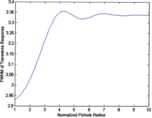
By solving these equations numerically for different pinhole sizes, a plot can

be constructed of the FWHM of the transverse response versus the pinhole size. An

example of such a plot can be seen in Figure 2. The regime for Type 2 confocal systems is

typically considered to be vp 0.5, and in the current setup the normalized pinhole radius

is approximately 6.4, well into the Type 1 confocal regime.

3.4

3.35

-3.3

0 3.25

£~3.2

S3. 15

3.1

3.05

3

2.951

1

2

3

4

5

6

7

Normalized Pinhole Radius

8

9

10

Figure 2: FWHM transverse response of a confocal system.

F

D. Temperature Gradient

The capillary plate in the scanning CGE system can be modeled as a thin plate

(or fin) with constant flux sources at either end and allowing for convective and radiative

losses across the length of the plate. The dynamic model is complex, and instead of

solving the physical model, an inverse mathematical model was created for the plate so

that a temperature gradient could be chosen and the appropriate voltages for each heater

could be set. The final model is 31d-order in the two temperature variables and takes the

following form,

V7(TT2)=a+a

T

+aT +aT

_{+a T T T+aT}

_+aT

0 1 1 2 2 3 1 4 1 2 5 2 6 1

+aT T2

+a

T T2+aT3

(7)

although a 2nd-order model could be used without much more error. Temperature data

was taken from the capillary plate at varying temperatures with voltages ranging from

2-14 V on the cold side to 2-18 V on the hot side, with the cold side heater having a lesser

or equal voltage than the hot side heater. The above model was then fitted to these data

using a Marquardt minimization routine. The Visual Basic code for this routine is given in

Appendix E.

Once the 3rd-order model was fit to the data, the model was evaluated at the

temperatures of the original data points and the errors between the model and data were

calculated. The statistics of the errors can be seen in the Table 1.

Error Statistics

Hot Side Heater Cold Side Heater

Mean Error

[VJ

6.759x10-14

3.109x10-1

St. Dev.

[V

9.380x10-2

0.2531

Min

[V

-0.2600

-0.3373

Max

[VJ

0.2046

0.5626

Vcold

VT4,

x

-

Measured

Data

U

30..

10

J.-10

...

0-Hot Side Temperature [*C]

80

4

s

20

20

40Cold Side Temperature

[

Figure 3: Cold side heater voltage as a function of temperature gradient.

V

=

V(T.

_h

T

_cold)

)

Measured

Data

80

1W

60..

40

Hot Side Temperature [*C]

20

20

CO

100

Id Side Temperature [*C]

Figure 4: Hot side heater voltage as a function of temperature gradient.

40,

200

160

1

50

I

-60

-100

-150

100

C]

40 - -- ',

30,

20-10,

0

I

_1-10

-20

-30

-40

-60

-70

The model curves and actual data are plotted in Figures 3 and 4. The model

should be approximately symmetric about the

THOT

=

TCOLD

line but it is not. However, no

data was taken to on the opposite side

(THOT

TCOLD)

to predict this part of the curve.

III. Experimental Design & Setup

A. Optical Subsystem

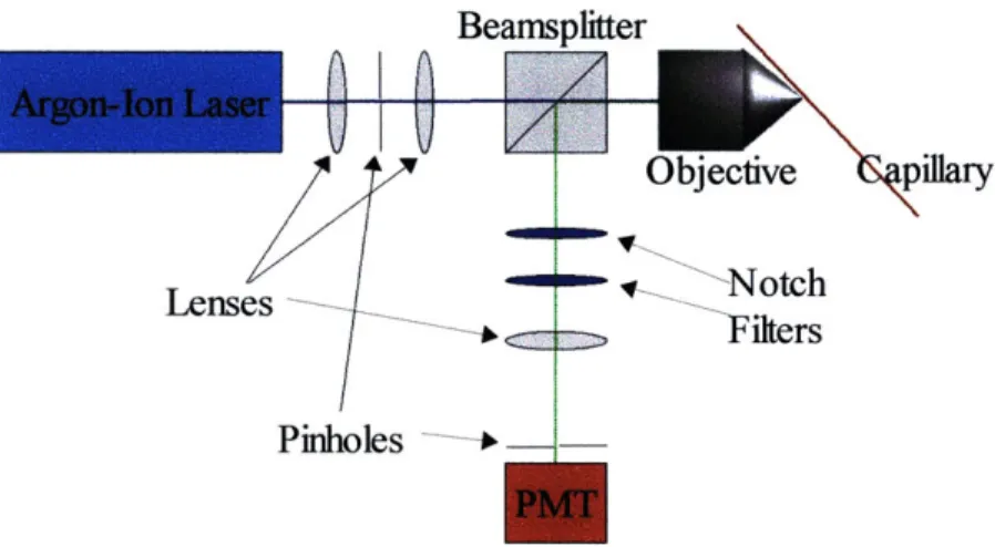
A Type II confocal optical system was used to detect the fluorescence

emissions from the tagged DNA in the capillary tube. The system consisted of an argon

ion laser at 488 nm, a series of lenses and pinholes, a beamsplitter cube, two laser "notch"

filters (Omega Optical, Brattleboro, VT), an objective and a small photomultiplier tube. A

diagram of the optical subsystem can be seen in Figure

5.

Beamsplitter

Objective

pillary

s NNotch

Lenses

_Filters

Pinholes

Figure 5: Optical subsystem schematic.

The laser was a refurbished Uniphase air-cooled argon ion laser (488nm) with

a maximum power output of 40 mW. All optics were mounted in an Spindler-Hoyer

optical framework, which provided precision and ease of use. Two plano-convex lenses

and a pinhole were used as a beam expander and as a spatial filter. The lenses had focal

lengths of 15 mm and 60 mm respectively, providing a beam expansion of 4x, and the

pinhole was 40 pm in diameter as was specified in Section IIC.

The expanded beam passed through a beamsplitter cube and into an lOx

objective (Olympus, Melville, NY). The fluorescent light from the capillary tube then

passed back through the objective and was reflected by the beamsplitter cube into the

detection portion of the system. The light first passed through two laser notch filters to

block any reflected light at 488 nm (T~Ix 10'). The light was then focused with a

plano-convex lens (f= 50 mm) through a second pinhole with a diameter of 100 pLm and onto

the Hamamatsu photomultiplier (PMT).

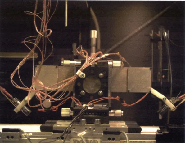
Figure 6: PMT and laser filter.

The nominal bandwidth of the Hamamatsu PMT was 20 kHz. The gain for

the PMT was controlled by an applied voltage ranging from 0-1 V, and was typically

operated with a gain of 0.75-0.95 V. The output of the PMT was passed through a series

of amplifiers and filters (See Section III E) to reduce noise and for interface with the PC

electronics.

B. Capillaiy Plate and Heaters

An aluminum plate was designed to hold the capillary and provided a steady

and linear temperature gradient across the length of the capillary. Copper blocks at each

end of the plate served as heat reservoirs. Each end of the plate was heated independently

by thin Joule heating elements on a Kapton

_{substrate (KHLV-202/1 0; Omega,}

Stamford, CT). A

375

jim wide groove was cut into the surface of the plate using

electro-discharge machining (EDM) techniques. The groove was used to hold the capillary so

that it maintained a more stable temperature profile. Small pieces of rubber were used at

either end of the plate to secure the capillary, which was press-fit into the groove.

Figure

7:

Capillary holder plate and alignment stages.

Adjustable plastic holders were attached at either end of the plate so that the

buffer vials were securely fastened to the frame. The whole capillary holder plate was

attached to a series of translational and rotational stages. The connection between the

first stage and the plate was made using acetyl standoffs and nylon screws to minimize

heat loss into the stages and to isolate the plate electrically. The stages consisted of two

orthogonally mounted translational stages (000-9141-01; Parker, Irwin, PA), and two

orthogonally mounted rotational stages (124-0055; OptoSigma, Santa Ana, CA). The

rotational stages were used to account for any misalignment in the rest of the mounting so

that the capillary could be made perpendicular to the optical axis and parallel to the

ground plane of the scanning stage. One translational stage, which was parallel to the

optical axis, was used to bring the system into focus, while the other stage was used for

transverse motion during scanning operations. Each translational stage was driven by a

microstepping motor (ZETA57-83-MO; Compumotor, Rohnert Park, CA) and controller

(ZETA6104; Compumotor) which was connected to the PC by a serial cable.

A series of twenty thermocouples (5TC-TT-E-36-36; Omega, Stamford, CT)

were distributed along the length of the plate to measure the temperature gradient. The

thermocouples were measured using an HP34970 data acquisition system and an HP34901

acquisition card set up to read thermocouples in degrees Celsius.

C. Capillary Interface

Syringe for

gas irjection

_Capillary

tube

Cap

Septum

Gel

buffer

ImL glass vial

High pressure injections were required to fill the capillaries with gel. The

injections were done with two different capillary interfaces. The first interface is pictured

below and uses a high pressure gas canister to push the gel into the capillary. The gas

used for the gel injections was typically argon or helium. The gel was injected at a

pressure of 1.

379x

_{105 Pa (20 psi). The valves controlling the gas for the gel injection}

were computer actuated to lessen introduction of contaminants into the system. Septa on

the sealed vials were pierced by disposable syringe tips through which the capillary was

fed to avoid coring. This method, however, did allow a significant amount of dirt to enter

the system, and could not provide enough pressure to pump the more viscous gels into the

capillary.

The second means of pumping gels into the capillary was by syringe injections.

A piece of TeflonTM tubing was secured over each end of the capillary tube. The tip of a

100 iL syringe filled with gel was then inserted into the tubing at one end. The

TeflonTM/steel interface provided a suitable seal for the injections. In this way, the

polymer gel was manually injected into the capillary tube.

UV Glue

_Epoxy

Syringe

_Capillary

Mf! Shrink

Teflon ubing

Direction of fluid injecti~n

Figure 9: Capillary high pressure syringe interface.

D. Capillaries & Gel Chemistry

The capillary tubes were purchased in spools from PolyMicro Technologies

(Phoenix, AZ). Two sizes of capillaries were used, one with an inner diameter (ID) of

75

provide strength and to prevent breakage. The outer diameter (OD) of the coated

capillaries was approximately

375

pm. Capillaries used in the CGE experiments were

typically

550

mm long, and the polyimide coating of the middle 100 mm was burned off

with a butane torch so that the fluid inside could be optically interrogated. The capillaries

were then filled with a viscous polymer gel which was used as the separation matrix for

the DNA.

Two separate series of chemistries were used to develop this setup. The first

was a proprietary gel mixture purchased from Coulter (477628;

Beckman-Coulter, Fullerton, CA). The second polymer gel chemistry was prepared in-house

roughly following the procedure described by Khrapko, et al. (1996).

The first gel was adequate for separating a standard DNA "ladder" but

problems arose when attempting to inject other DNA. It was decided that a gel produced

in house would provide more control over the gel characteristics as well as being cheaper

to produce. First the capillaries were washed with 1 M NaOH for 2 hours. Then they

were washed sequentially with 1 M HCl and methanol. Afterwards, the capillaries were

filled with y-methacryloxypropyltrimethoxysilane and left overnight. Then the capillaries

were washed again with methanol, and a 6% acrylamide gel solution in Ix TBE, 0.1%

TEMED, and 0.025% ammonium persulfate, was injected into the capillary and left for 30

minutes to polymerize. This gel was then pumped out to prevent clogging the capillary

and a

5%

acrylamide gel solution in Ix TBE, 0.03% TEMED, and 0.003% ammonium

sulfate was injected into the capillary for separating the DNA. This gel was replaced with

new gel after every run. During the runs the capillary ends were submerged with the high

voltage electrodes in a vial of the running gel.

.0

a)a

.00

350

400

450

560

550

600

650

700

Wavelength (nm)

Figure 10: Absorbance and emission spectra of YO-PRO-1 (taken from Molecular Probes, Inc.).

The DNA was tagged with a fluorescent intercalator, YO-PRO- 1 (or oxysol

yellow) purchased from Molecular Probes (Y-3603; Molecular Probes, Eugene, OR).

This molecule, as was mentioned above, fluoresced proportional to the amount of dsDNA

to which it was bound. Ethidium bromide (E-1305; Molecular Probes), another

fluorescent intercalator, was used in some early runs, but YO-PRO- 1 was known to have

a better response as the dsDNA melted (Hogan, 2000). The absorbance peak of

YO-PRO-I is at 491 nm and the emission peak is at 509 nm. The absorbance and emission

spectra of YO-PRO-1 when bound to dsDNA can be seen in Figure 10.

For some runs of DNA in temperature gradients, a denaturant, nicotinamide,

was added to the gel buffer before polymerization. The denaturant was used to lower the

melting temperature of the DNA segment to a range more amenable to good

signal-to-noise ratio in the CGE scanning system.

E. Electrical Subsystem

The electrical subsystem of the CGE system is shown in Figure 11. The

electrical subsystem consists of two programmable triple output power supplies

(HP363 1A; Hewlett Packard, Palo Alto, CA), three programmable single output power

supplies (HP3632A; Hewlett Packard), one high voltage power supply, (CZE1000R;

Spellman, Hauppauge, New York), a series of intermediate electronics and a data

acquisition board (Allios board, MIT Bioinstrumentation Lab) that was produced

in-house. The HP power sources provided all power for intermediate electronics, for the

PMT, and for heating the capillary plate. The HP sources were controlled by a PC

through a IEEE 488 connection using a National Instruments IEEE 488 interface board.

The CZE1 OOR had a maximum output voltage of 30 kV and a maximum

output current of 300 pA. Polarity could be controlled on the front panel, but this option

was modified so that the polarity could be controlled by an applied voltage to the terminal

block on the back of the device. High voltage and the current limit on the device were

also set by applying voltages to the terminal block. Actual current and high voltage values

were monitored off the terminal block. All voltage inputs and outputs to the terminal

block ranged from 0 V to 10 V. To interface these inputs and outputs to the PC's data

acquisition board the voltages were scaled to the proper voltage ranges. Outputs from the

CZE1000R were scaled down by a factor of 2.2 using a simple voltage divider, and the

outputs from the Allios board were amplified by a factor of 3.3 using a simple

non-inverting amplifier (see Appendix B).

The gain of the Hamamatsu PMT was changed by a 0-1 V control voltage

which was applied by one of the HP363 lAs under computer control. The PMT outputted

a current which was first changed into a voltage by a simple current amplifier circuit. The

current amplifier converted from 0-100 pA to 0-4 V with a bandwidth of 20 kHz. The

voltage signal was then passed through a 2n-order Butterworth filter to reduce high

frequency electro-magnetic noise, including electrical line noise. The cutoff of the

Butterworth filter was 43 Hz with a DC gain of 1.597. These values were measured with

a Hewlett-Packard Dynamic Signal Analyzer (HP3562A, Hewlett-Packard). The phase

and gain frequency response plots of these two components can be seen in Appendix B.

Amplifiers

& Voltage

CZE1000R HV

Diviers

---Heavy Black Lines: Power Connections

Thin Red Lines: Signal Connections

Figure 11: Electrical subsystem schematic.

F. Computer Automation and System Operation

Operation of the setup was automated through the use of a personal computer

(PC) and Visual Basic (VB) programming. The PC had a

450

MHz Pentium II processor,

384 MB of RAM and ran the Microsoft Windows NT 4.0 operating system. All Visual

Basic programming was done with Microsoft Visual Basic 6.0 and compiled for increased

speed. All HP devices were controlled through their IEEE 488 ports using a National

Instruments IEEE 488 interface card in a PCI slot. The National Instruments board was

accessed by Visual Basic through Visual Basic Class Modules which were built on top of

the basic National Instruments VB interface. The Allios data acquisition board, which

resided in one of the PC's PCI slots, was accessed through a Visual Basic Class Module

which was built on top of a specially written WinRT

_{dynamic linked library (DLL).}

The CGE system was programmed to operate in two different modes, Simple

Run and Simple Scan. In Simple Run mode, the plate remained stationary while the CGE

run was performed and temperature was not recorded. The user was able to set the

sample rate, the total number of samples, the applied high voltage, the current limit, and

the PMT gain voltage. In Simple Scan mode, the plate was scanned back and forth and

the user was given the option of recording the temperature of the plate at the end of each

scan. The user was also able to set the following parameters (with typical running values

in parentheses): length of scan (100 mm), time for scan (10 s), sample rate (10 Hz),

number of scans (1000 or 1800), high voltage (5.5 kV), current limit (100 pA), and PMT

gain voltage (0.75-0.9 V). At the end of each scan the plate motion paused to allow for

temperature readings from the twenty thermocouples and for resynchronization with the

program.

After each data collection, the data was saved in text files on the hard drive

which could be imported into MATLAB or some other data analysis program. A typical

run consisted of electrokinetically injecting fluorescently tagged DNA into the capillary

and then switching the cathode solution back to the buffer gel and running for several

hours. The DNA was injected at a field strength of 20 V/mm for 90 s while recording

data at 100 Hz in the Simple Run mode with the PMT gain voltage set to 0 V. The plate

was then aligned perpendicularly to the optical axis and run in Simple Scan mode.

G. System Mounting and Housing

The entire CGE system was mounted onto an optical bench with built-in

vibration isolation (2"d-order lowpass with a cutoff of ~1 Hz) which was then floated on

air bearings (TMC, Peabody, MA). To further minimize vibration, the cooling fan from

the laser was removed from the laser head. Ductwork was then installed to provide

proper cooling while transmitting significantly less vibration.

Due to the sensitivity of the PMT detector, experiments were performed in

darkness. An outer housing for the setup was constructed from 45 mm (13/4") square steel

beams (Unistrut, Woburn, MA). This framework was covered with corrugated black

plastic (AIN Plastics, Norwood, MA) and sealed with black vinyl tape to provide a

light-tight box.

IV. Results

A. Simple Run

2

1.8

1.6

1.4

-c

1.2-0.81

0.6

RunO2 01-26-2000

20

40

60

80

100

Time [minutes]

120

140

10

180

Figure 12: Simple run data.

As was mentioned above, during the Simple Run mode of operation of the

experimental setup, the stage was kept stationary and temperature was not recorded. The

Simple Run mode typically was used to load the capillary electrokinetically before a

Simple Scan experiment. When loading the capillary, the PMT gain was set to 0 V, or no

gain. The Simple Run mode was also used initially to test new mixtures of DNA and

fluorescent molecules because the Simple Run mode was more easily aligned than the

Simple Scan mode. Data from a Simple Run can be seen in Figure 12. The DNA in this

run consists of a standard "ladder" tagged with ethidium bromide.

1

2

3

4

5 6

0.4'

0

I

I

-"0

The peaks seen are the first seven bands of the DNA ladder. The sample in

this run was electrokinetically injected for 90 seconds at 10.6 kV for a field strength of 20

V/mm. The PMT signal was sampled at 2 Hz for 3 hours and DNA was run also run at a

potential of 10.6 kV. The PMT gain was set at 0.9 V. After the run, a 3-point median

filter was applied to the data to eliminate single point noise spikes. The peaks in this plot

correspond to the following DNA segment lengths (all lengths give in basepairs or bp): 72,

118, 194, 234, 271, 281, and 301.

B. Simple Scan

Using the Simple Scan mode, data could be taken across the length of the

capillary rather than at just one point. Due to the dynamic nature of this mode, the

alignment procedure was much more important. Small misalignments often resulted in

wide fluctuations of the background noise and decreases in the S/N ratio. Said

misalignments most often were the result of the scanning axis not being completely parallel

to the capillary. Once the proper alignments were completed, though, the signal and

background were quite consistent across the whole scanning length.

Figure 13 shows a Simple Scan of both standard ladder DNA and the SNP

DNA sample would possibly have a SNP. The sample DNA and the DNA standard were

mixed into a solution at approximately equal concentrations, but because the DNA

standard had 11 bands, the amount in each of its band (and therefore the brightness) is

significantly less than the SNP sample band, which is obviously brighter than the others.

In the figure the scans are taken along the vertical axis and time along the

horizontal axis. Due to a constant delay caused by the finite acceleration of the linear

stages, the anti-parallel scans had to be slightly shifted to align the picture. In the Simple

Scan shown in Figure 13, the even and odd scans were shifted by a total of 6 data points.

This value was determined by trial and error and was perfected by aligning the constant

features in the image. A 3-by-3 median filter was applied to the raw data to eliminate

single points of noise so that a proper range expansion could be done. This run was done

without turning on the heaters and served as a temperature "standard" for later runs with a

temperature gradient.

RunO2 03-23-200

10

E

cc

ro

80

70

60

50

40

30

20

10

50

100

150

200

250

300

350

Time [minutes)

Figure 13: Simple scan data.

As could be seen in the Simple Run shown above, the

5'

and 6' bands are

quite close together, but could still be discerned with a stationary detector. In the Simple

Scan plot the

5'

_{band is approximately twice the brightness of the other ladder bands.}

This suggests that the real

5'

_{and 6' bands were unresolveable in this run.}

C. Gradient Scan

After the system was properly calibrated and aligned by doing Simple Scans,

the heaters at either end were powered to apply a specified temperature gradient across

the length of the plate. The values for either end of the temperature gradient were chosen

first and then the formula described in Section III D was applied to find the approximate

voltages to be applied to the hot and cold side heaters.

Then the plate was aligned as described above and DNA was injected. Gradient Scans

were run with similar parameters as Simple Scans except that the number of scans was

increased (up to 2300) to account for the DNA slowing once it was melted.

Rur2 03-27-2XNO

10

E

i,

C

80

70

60

50

40

30

20

10

50

100

150

200

Time

[minutes]

350

Figure 14: Gradient scan data.

Figure 14 shows a Gradient Scan with both the DNA ladder and the DNA

SNP sample. Multiple bands can be seen to change velocity during the course of the run.

Also, the peaks can be seen to broaden as they slow, possibly a result of the higher

temperatures contributing to faster diffusion. Because there are so many bands from the

ladder and because no single band stands out as brighter than the rest, identification of the

SNP DNA is difficult. In this particular run the gel buffer did not contain nicotinamide,

and in general, the runs with nicotinamide (at 1.5 M) were very poor and did not show any

V. Analysis

A. DNA Velocities

The fact that larger DNA fragments should move through gels more slowly

than small DNA fragments is the basis for all of CGE work. This can be confirmed

through more in depth analysis on some of the resultant data. The bands in Figure 13

provide a clear data set with which to work, although all of the successful Simple Scan

data sets would provide similar information.

To measure the velocities of each peak, the data set was broken into regions in

which there was only a single band. Then, the scan during which each position along the

capillary had its maximum was calculated. This was found to be a good measure of the

position of the center of each peak. A straight line was then fit to each data set with the

slopes of the lines equal to the respective velocities of the peaks. It was necessary to

reduce the amount of data available to the fitting routine for some of the DNA segments

due to close bands corrupting the peak finding calculations. With more sophisticated peak

finding algorithms, this manual step could be eliminated and the velocity estimates

improved.

The velocities of DNA bands can be seen plotted in Figure 14 along with the

fitted model. The model is a simple exponential with the form,

v(l)=eal'I+a

+a3 ,

(8)

and was fitted to the data using the Marquardt minimization routine listed in Appendix E.

For this data set, the fitted parameters are listed in Table 2, and the

percent-variance-accounted-for (%VAF) of the model was calculated to be 99.988%. Then, according to

Equation 2, for a constant voltage the velocity is inversely proportional to the viscous

drag coefficient. Therefore, the drag coefficient must have a exponential relationship to

DNA segment length.

a,

a

a

-0.003437

-1.827866

0.094323

200

600

600

DNA length [bp]

1000

1200

140

Figure 14: Velocity vs. DNA Length.

B. Denaturant

The denaturant, nicotinamide, was added to the acrylamide gel before

polymerization to lower the melting temperature of the DNA segments. However, the

denaturant seemed to interrupt the polymerization processes, and the resulting buffer was

not suitable for electrophoresis.

A denaturant is desirable in the current setup for several reasons. First, as the

aluminum capillary holder plate heats, it will expand and cause the plate to move out of

alignment, and getting consistent data becomes much more difficult. Also, as the fluid

inside the capillary heats, the viscosity and thus the efficacy of the polyacrylamide gel

changes. This causes nonlinearities in the separation and makes velocity changes of the

DNA bands more difficult to identify and quantify. By lowering the melting temperature

of the DNA strands, the system can be moved away from the regime where these

0.22

0.2

-

Exponential Fit

E

0.

0.

0.

18

16

14

12

0.1

200

nonlinear effects become significant. Nicotinamide, as yet, does not seem suitable for use

in gels, and other denaturant choices should be pursued.

C. Curve Tracking and Identification

RunOl 03-31-200

90

80U

E

C

70

60

50

40

30

20

10

50

100 150

200

250

300

350

400

450

Time

[minutes]

Figure 15: Gradient scan with single DNA band.

As can be seen in Figure 14, analyzing many DNA peaks in one gradient scan

is complicated. The curves for each ladder peak confound the identification of the SNP

DNA peak, and ideally the system would be run with the DNA ladder. However, in

experiments where only the SNP DNA was run in the CGE system (Figure 15), the

migrating band did not experience the expected velocity shift. The slight shift which did

occur also came at a higher than expected temperature. This suggests that either the

temperature sensors do not reflect the actual temperature within the capillary or that the

high temperatures are affecting the interaction between the DNA and the polymer gel.

VI. Conclusions

The scanning confocal CGE system provides a new way to obtain information

about CGE systems. This technology also allows CGE systems to be run in new ways that

could dramatically affect the discovery, analysis and screening of SNPs. Future

configurations could also take greater advantage of the CGE technique's ease of

automation to produce a system for mass scale SNP screening.

Current data from the CGE system does not show the expected DNA velocity

break in the thermal gradient, however the results are promising. Lowering the overall

required temperature through the use of denaturants is one aspect of the project that

should continue to be pursued. Not only will the gel be more predictable at lower

temperatures, but as much of the data has shown, the signal-to-noise ratio seems to be

better at lower temperatures.

Efforts are currently being made to use feedback control for tracking

individual peaks as they travel through the capillary rather than simply raster scan across

the capillary's length. This technique, once perfected, should provide additional increases

in signal to noise ration by sampling more often around the peaks rather than in areas of

no interest. Tracking peaks should also allow the linear stages to move more slowly and

thus more smoothly, eliminating some of the noise from mechanical vibrations.

In the next iteration, much consideration should be given to the capillary plate

and interface as well as the entire temperature measurement system. Capillary alignment

was a critical and time consuming step which had to be performed before every

experiment. A better mounting system would immediately speed setups times and

improve data quality. The decision to use thermocouples for measuring the temperature

gradient in the plate should also be revisited. Mounting the thermocouples so that they

produced accurate and repeatable data was not an insignificant task. With a better

theoretical model for the temperature gradient in the plate, fewer and more accurate

temperature probes might be used to measure the temperature data.

VII. References

Angel, A. DNA Mutation Detection via Electrophoresis: Thermal Gradient

Development. S.B. Thesis, Department of Mechanical Engineering, MIT, Cambridge,

MA: 2000.

Bioinstrumentation Lab, MIT, Cambridge, MA. http://biorobotics.mit.edu/.

Brookes, A. J. Gene. 1999, 234: 177-86.

Camilleri, P., Ed. Capillary Electrophoresis: Theory and Practice. CRC Press, Boston:

1998, 91-105.

Doukoglou, T. D. Theory, Design, Construction and Characterization of Confocal

Scanning Laser Microscope Configurations. Ph.D. Thesis, Department of Electrical

Engineering and Department of Biomedical Engineering, McGill University, Montreal,

Quebec, Canada: 1995.

Foret, F., L. Krivankova, and P. Bocek. Capillary Zone Electrophoresis. VCH, New

York: 1993, 41-8.

Gille, C., A. Gille, P. Booms, P. N. Robinson, P. Nrnberg. Electrophoresis. 1998, 19:

1347-50.

Grossman, P. D., and J. C. Colburn, Eds. Capillary Electrophoresis: Theory and

Practice. Academic Press, Inc., New York: 1992, 14-24.

Hogan, C. Personal communication. Department of Biology, MIT: 2000.

Horowitz, P. and W. Hill. The Art of Electronics,

2n

Ed. Cambridge University Press,

New York: 1989.

Human Genetic Bi-Allelic Sequences (HGBASE). http://hgbase.interactiva.de/.

Karger, B. L., Y.-H. Chu, and F. Foret. Annu. Rev. Biophys. Biomol. Struct. 1995, 24:

579-610.

Khrapko, K., H. Coller, and W. Thilly. Electrophoresis. 1996, 17: 1867-74.

Lerman Lab, MIT. Cambridge, MA. http://web.mit.edu/biology/dna/.

Lerman, L. S. Personal communication. Department of Biology, MIT: 2000.

Lide, D. R., Ed. CRC Handbook of Chemistry and Physics,

73'd

Ed. CRC Press, Ann

Arbor: 1992.

Molecular Probes, Inc. Eugene, OR. http://www.molecularprobes.com/.

National Center for Biotechnology Information, dbSNP. Bethesda, MD.

http://www.ncbi.nlm.nih.gov/SNP/ndex.html.

Press, W. H., S. A. Teukolsky, W. T. Vetterling, and B. P. Flannery. Numerical Recipes

in C: The Art of Scientific Computing,

2"

Ed. Cambridge University Press, New

York: 1992.

Ruiz-Martinez, M. C., J. Berka, A. Belenkii, F. Foret, A. W. Miller, and B. L. Karger.

Anal. Chem. 1993, 65: 2851-8.

Stenesh, J. Biochemistry. Plenum Press, New York: 1998.

Watson, J. D., and F. H. C. Crick. Nature. 1953, 171: 737.

Wilson, T., Ed. Confocal Microscopy. Academic Press, New York: 1990.

Wilson, T. and C. Sheppard. Theory and Practice of Scanning Optical Microscopy.

Academic Press, New York: 1984.

Appendix A: MATLAB* Code

function a

segment(data,scans, lag)

segment.m

Written by Matthew R. Graham

Last modified on 18 April 2000.

2000 Copyright Matthew R. Graham and Bioinstrumentation Lab.

Converts single column of interlaced data to 2D array of data which

can be have every other row shifted to compensate for a constant lag

in a standard raster scan. Inserts mean of data into empty entries

where the lag shift takes place.

s

=

size(data);

scanlength

=

s(l)

/

scans;

mn

=

mean(data);

for m

=

1

:

scans

if (lag > 0)

if

(mod(m,2)

==

1)

a(l:scanlength,m)

=

_{data((m-l)*scanlength + 1:m*scanlength);}

a(scanlength+l:scanlength+lag,m)

₌

_{ones(lag,1)*mn;}

else

a(1:lag,m)

=

ones(lag,1)*mn;

a(lag+1:scanlength+lag,m)

=

data(m*scanlength:-l:(m-1)*scanlength + 1);

end

else

if

(mod(m,2)

==

1)

a(:,m)

=

data((m-1)*scanlength + 1:m*scanlength);

else

a(:,m) =

data(m*scanlength:-l:(m-1)*scanlength + 1);

end

end

end

function f

platemodel(ht,ct,p)

platemodel.m

%

Written by Matthew R. Graham

Last modified on 18 April 2000.

2000 Copyright Matthew R. Graham and Bioinstrumentation Lab.

Applies 3rd order model for heating of capillary plate.

Inputs: Hot Side Temperature, Cold Side Temperature,

and (Hot or Cold) Model Parameters.

Outputs: (Hot or Cold Side Heater) Voltage necessary.

f

=

_{p(1) + p(2)*ht + p(3)*ht^2 + p(4)*ct + p(5)*ct^2 + p(6)*ht*ct}

₊

function f

=

trackmax(data)

trackmax.m

Written by Matthew R. Graham

Last Modified on 25 April 2000.

% 2000 Copyright Matthew R. Graham and Bioinstrumentation Lab.

Returns position of maximum value across length of array.

s

size(data);

1

for i

=

1:1

[x,f(i)I

max(data(i,:));

end

function f

unwind(p)

unwind.m

Written by Matthew R. Graham

Last Modified on 29 April 2000.

%

_{2000 Copyright Matthew R. Graham and Bioinstrumentation Lab.}

Unwraps phase data from HP3562A taken through HPVEE programming.

pl

=

flipud(p);

p2

=

pl.*pi./90;

p3

=

unwrap(p2);

p4

=

p3.*90./pi;

f

=

flipud(p4);

Appendix B: Electrical Diagrams

V

R

₃

out

R

Figure Bi: Voltage di-vder.

LTI001

15 V

V.

+

15 V

R 1

100

nF

53.1 kQi 53.1 k

TIO

1

V

n-v

out

100

-15

V

31.6 k

g53.1 kQ

Figure B2:

2nd

order Butterworth filter.

out

Figure B3: Voltage amplifier.

200 pF

40 kM

AD549

_{15 V}

-15 V

V

(a) Amplifier Gain Plot

0F

10

1re

I

d

10

10

Frequency [HzI

(c) Fifter Gain Plot

20

0

01

CL

I'

(b) Amplifier Phase Plot

4A0[

4M

h

10

0

-c

0~

0

10,

10

l

0

1

Frequency jHzJ

(e) Amplifier & Filter Gain Plot

10

102

10,

Frequency [Hz]

10

10

(d) Filter Phase Plot

-100

-150

100

0

CL

0f

10'

102

1

o1

106

Frequency

[HzI

-100

-150

-2M

101

11

10

3

le

Frequency [Hz]

(f) Amplifier & Filter Phase Plot

106

I00

10'

i02

10'

d

Frequency [Hz]

Ngure

B5: Phase and magnitude plots for filter and amplifier.

10i

I

ta

10

1

102

0

1o

1-1

102

1(r

1

0

210

I

00

Appendix

C:

Mechanical

Drawings

I+1~

1.~

I

II1

io

31~

2

a

I

E

z

---Figure

Cl:

Capillary

plate

mechanical

schematic

(taken

from

Angel,

2000).

38

-+

Thermal Reservoir Plates

Thermocouple Jig

_

Thermocouple Trough

-

Capillary Trough

Gradient Plate

Figure C2: Capillary plate and vial holders mechanical drawing (taken from Angel, 2000).

Vial