Development and experimental validation of a predictive model for a GTA weld pool geometry

DEVELDPMENT AND EXPERIMENTAL VALIDATION OF A PREDICTIVE MODEL FOR A GTA WELD POOL GECMETRY

by

GEORGE EMK ARNIADAKIS

Engineering Diploma in M.E. and N.A.M.E. NATIONAL TECHNICAL UNIVERSITY OF ATHENS, 1982

Submitted to the Department of Mechanical Engineering in Partial Fulfillment of the Requirements of the Degree of

MASTER OF SCIENCE IN MECHANICAL ENGINEERING at the

MASSACHUSETTS INSTITUTE OF TECHNOLOGY

June 1984

EGeorge Em Karniadakis

The author hereby grants to M.I.T. permission to reproduce and to distribute copies of this thesis document in whole or in part.

Signature of Author:

Departmentvof Mechanical Engineering

Certified by:

A

Thesis Suprvisor

Accepted by:

hA A A/ 1 l - v -/v

Chairman, Mechanical Engineering Departmental Comnittee

ARCHIVES

MASSACHUSETTS INSTiTUTE OF TECHNOLOGY

OCT 0 2 1984

2

DEVELOPMENT AND EXPERIMENTAL VALIDATION OF A PREDICTIVE MODEL FOR A GTA WELD POOL GEOMETRY

by

GEORGE EM KARNIADAKIS

Submitted to the Department of Mechanical Engineering in partial fulfillment of the

requirements for the Degree of Master of Science in Mechanical Engineering

ABSTRACT

A computationally simple, but physically based model has been developed to predict the geometry of stationary weld puddles. The overall model couples a weld pool rodel that includes convection of the nolten metal to a heat conduction solution for the solid material to obtain a predictive technique for the fusion boundary. Electroragnetic, surface tension and plasma shear forces are considered in determining the flow pattern in the weld pool. Direct comparison of predicted parameters with experimental data show a very good agreement, especially when the (radiative) heat losses from the plate surface are included. Experiments were also taken to determine the arc efficiency, and an empirical formula was found to correlate the heat input to the workpiece to the power dissipated in the electrode. While additional

validation of the model is desirable, the basic approach has been shown to be good and the techniques can now be applied to the transient response of

stationary puddles and to the full welding situation.

Thesis Supervisor: Dr. William Unkel

CHAPTER TITLE PAGE ABSTRACT TABLE OF CONTENTS LIST OF FIGURES ACKNOWLEDGEMENTS 3 TABLE OF CONTENTS PAGE 2 3 5 8 1 1 .1 1.2 1.3 INTRODUCTION PREVIOUS RESEARCH

SCOPE OF THE PRESENT RESEARCH

2 THE FULL PROBLEM FOR A GTA WELD PUDDLE

3 3.1 3.2 3.3 3.4 3.5 3.6 3.7 3.8 EXPERIMENTAL APPARATUS

EXPERIMENTS AND RESULTS ON THE ARC V-I CHARACTERISTICS EXPERIMENTS AND RESULTS ON ARC EFFICIENCY

TEMPERATURE MEASUREMENTS VELOCITY MEASUREMENTS CROSS WELD SECTIONS MEASUREMENT OF T SUMMARY 4 THEORETICAL ANALYSIS 4.1 INTRODUCTION 9 12 14 16 19 24 28 37 46 48 51 52 53 1

4

TABLE OF CONTENTS (continued)

CHAPTER PAGE

4.2 CONDUCTION IN THE SOLID 55

4.2.1 FINITE ELEMENT MESH EMPLOYED 55

4.2.2 HEAT FLUX CALCULATIONS 61

4.2.3 TOP SIDE TEMPERATURE SENSING 62

4.3 CONVECTION IN THE WELD POOL 67

4.3.1 ELECTROMAGNETIC DRIVEN FLOW 67

4.3.2 SURFACE TENSION DRIVEN FLOW 70

4.3.3 PLASMA STREAM SHEAR FORCE 72

4.3.4 BUOANCY FORCE 72

4.3.5 VELOCITY FIELD 72

4.3.6 FLOW STRUCTURE: Two and Three parareter model 73 4.4 TEMPERATURE FIELD IN THE WELD POOL 75 4.5 MATCHING OF CONDUCTION/CONVECTION SOLUTION 78

5 5.1 PREDICTED WELD POOL GEOMETRY 80

5.2 COMPARISON OF RESULTS PREDICTED BY THE MODEL 88 WITH EXPERIMENTAL DATA

6 SUMMARY, DISCUSSION AND RECOMMENDATIONS 93

REFERENCES 96

APPENDIX A-ELECTROMAGNETIC FORCE J x B 98 APPENDIX B-A SIMPLE SOLUTION TO THE 2-D STEADY 101

THERMOCAPILLARY MOTION

APPENDIX C-STAGNATION FLOW 104

5 LIST OF FIGURES

FIGURE PAGE

NUMBER NUMBER

1 . Schematic of Overall Strategy for Smart Welder 11 2. The full problem for a GTA weld puddle 17

3. The electric circuit 18

4. Overall view of arc welding experimental set-up 20

5. The workpieces tested 21

6. The copper plate base 22

7. Schematic of the current regulator showing the protection

and sequencing circuit 23

8. Effect of arc length on the V-I curve 26 9. Effect of puddle formation on the V-I curve 27

10. Calibration of flowmeter 30

11. Effect of flow rate on arc efficiency 31 12. Effect of arc length on arc efficiency 32

13. A universal curve for the arc efficiency 34

14. Effect of current pulsing on arc efficiency 35 15. Effect of flow rate on topside temperature 39 16. Centerline back temperature for different arc lengths 40 17. Centerline back temperature for different workpieces 41 18. Topside temperature versus effective heat input 43 19. Back temperature versus effective heat input 44 20. Effect of current pulsing on the c-1 back temperature 45

6

LIST OF FIGURES (continued)

FIGURE PAGE

NUMBER NUMBER

21a Shallow puddle for workpiece 7/8"t*7/16" 49 21b Full penetration for workpiece 7/8"?*7/32"1 49

22a Parabolic boundary 50

22b Double shape boundary 50

23a Demonstration of axisymmetric conditions 56

23b Reduction to half width geometry ₅₆

24. FEM mesh employed with a parabolic boundary 57

25. FEM mesh employed with a parab+elliptic boundary 58

26. FEM mesh for the three parameter model 59

27. An improved FEM mesh with 32 isoparametric elements 60 28. Comparison of heat fuxes for different pool aspect ratios 63 29. Comparison of adiabatic and heat radiated plate surface 64

30. Comparison of different boundaries 65

31. Top temperature sensing 66

32a Motion induced by the em magnetic field 69 32b Idealized system for the em driven flow 69

33a Two parameter model 74

33b Three parameter model 74

34. Convection heat transfer calculations 77

35a Current pulsing developed weld puddles 81

35b Direct current developed weld puddles 81

36. Predicted and measured penetration 82

7

LIST OF FIGURES (continued)

PAGE NUMBER

84

85

86

38. Predicted and measured penetration for thick workpiece 39. Predicted and measured width versus penetration

40. Predicted centerline back temperature 41. Predicted top temperature

42. Comparison of predicted and measured c-i back temperature (Adiabatic conditions)

43. Comparison of predicted and measured top temperature (Adiabatic conditions)

44. Comparison of predicted and measured back temperature (Adiabatic conditions)

45. Comparison of solutions corresponding to different plate surface boundary conditions

46. Surface tension driven flow 47. Stagnation flow 90 91 92 103 103 FIGURE NUMBER

8

ACKNOWLEDGEMENTS

I would like to acknowledge with gratitude the assistance of my advisor, Professor William Unkel, in giving direction and encouragemnt to my

endeavors.

This work was funded by the Department of Energy, Contract No. DE-ACO2-83ER 13084.

9

CHAPTER ONE 1.1 INTRODUCTION

Welding is a metal joining process that has broad application in a variety of constructions and repair operations. While simple welds can be made by moderately skilled welders, high quality welds require very skilled welders and must pass stringent inspection criteria. Even a small fraction of

faulty welds can cause a substantial increase in the overall cost of welded structures. Producing high quality welds consistently is a major goal of welding research.

The work described in this thesis relates to the behaviour of the molten pool, in particular to the thermal (heat transfer) and fluid (stirring) response of the molten metal during the fusion process. This work has been performed in the context of developing an automatic or "smart" welder that controls directly the weld attributes that lead to a high quality weld. Thus,

this smart welder requires not only a manipulator to position the torch and controls the weld arc, but also requires a system to determine the proper position, current and other parameters.

This work focuses on Gas Tungsten Arc Welding (GTAW) a welding fusion process widely used for fusing the root butt joints, where exceptionally high quality is essential e.g. stainless steel piping for nuclear engineering applications. Other materials for which GTAW is suitable are : mild steels, low alloy steels, aluminum and aluminum alloys, copper and copper alloys, nickel and nickel alloys. In GTAW an arc is established between a tungsten electrode and the parent metal forming a weld pool. A non-melting electrode is used, usually made of thoriated tungsten, which gives better arc stability

10

and higher current capacity than ordinary tungsten. The electrode holder (torch) must be either air or water cooled and the power source can be a.c. or d.c. with standard generators, rectifiers or transformers.

Closed-loop control of the welding variables (current, voltage, torch speed, arc length,etc) represents a promising, cost effective approach to improving weld quality and therefore reducing the total cost of producing welded stuctures. The ultimate goal is to place all significant weld

variables under direct closed-loop control such that they depend only on the predetermined desired weld characteristics. The desirable weld

characteristics are pre-determined from strength and practical considerations for each particular structure. In addition to those charecteristics, closed-loop control requires four components:

(a) An on line technique for sensing each control variable;

(b) A physically based but computationally simple model relating the weld variables to the process inputs;

(c) At least one control variable on the welding device for each weld variable being controlled; and,

(d) A control algorithm that combines the above components to provide independent output variable control.

A functional sketch of a proposed automated control system is shown in Figure 1. The approach uses inner loops nested within the overall "weld quality" control loop. For example, the inner loop would be the torch/power

supply with control parameters those of current, arc length and torch speed (for moving torch). The control of the arc is achieved by a transistor controlled power supply, which is in itself controlled by a computer. The outermost loop is the weld quality loop, where the weld pool depth and width are sensed and the control variables are adjusted to keep these parameters close to the desired ones.

11

DESIRED WELD

CHARACTERISTICS

HEAT

WORK

WELD

.07

SOURCE

OKPIECE

CONTROLLER

PIECE

INNER LOOP

OUTER LOOP

12

1.2 PREVIOUS RESEARCH

The importance of predicting the temperature in and around the weld pool has long been recognized and considerable effort given to the task of

developing models. The early methods for calculating the geometrical

dimensions of the weld pool were based on the assumption that the mode of heat transfer through the plates was pure conduction. By assuming a linear

temperature distribution along the thickness of the liquid interlayer (from the boiling point at the surface adjacent to the heat source to the melting point at the fusion boundary) the thickness of the liquid interlayer could be inferred for a certain heat input. The major theoretical contribution on heat flow in welding was made by Rosenthal [1], who applied solutions of the heat conduction equation in two and three dimensions with a moving heat source. This solution in its simplified version as it was given by Wells [21 relates the average fused area width d, with the total heat per unit width q of the plate as follows:

q=8-k-AT-(0.2+U-d/(4-a))

where k,a are thermal conductivity and diffusivity of the solid respectively, AT is the temperature difference between the melting temperature and the surroundings and U is the velocity of the torch relative to the workpiece.

The predicted weld pool size, by the above analysis, has been found to differ by as much as 2-3 times [3] the size measured from experiments. The most probable explanation for this discrepancy is that in this analysis no allowance has been made to account for the enhanced heat transfer in the pool due to motion of the molten metal. One way to include this enhanced heat transfer is to use an effective isotropic or anisotropic conductivity to take care of directionality of heat in the pool or to introduce distributed heat sources or sinks. These techniques, however, have proved to be of very limited

13

use even to correlate the results. For example, Glickstein [4] found, after an extensive comparison of theoretical with experimental results and by using conductivities in the liquid region two to three times higher than the

conductivity of the solid material at high temperatures, that simulation of heat flow in the weld puddle for arc welding cannot be carried out using an exclusively conduction model. Although this conclusion was for a stationary puddle no difference should be expected for moving welds. While several such techniques are used, in some cases, to match the computed fusion boundary to measured contours, these ad hoc techniques are not predictive and can be used only as interpretive tools, but not in new situations under different welding conditions.

Woods and Milner [5] , in 1971, first reported that motion of the molten metal exists in GTAW pools and examined the origin of the stirring forces by partialy mixing dissimilar metals and concluded that stirring forces are not always sufficient to overcome basic incompatibilities in the physical and chemical properties of the weld pool and additives. In parallel, analytical work to study flows induced by electromagnetic forces was initiated by Shercliff [6] in 1970. In this first work a concentrated electric current entering a region of inviscid conducting fluid through an interface was

considered and an analytical solution was obtained for the non-linear equation of motion. Sozu [7] and others [8] solved similar problems, but for fluid with finite viscosity and their work has been extended to different geometries and configurations.

These solutions give the general features of free jet type flows for gases, and have been useful in identifying order of magnitude speeds.

Unfortunately the flow field in the pool turns out to be much more complex,and other driving forces, besides the electromagnetic force give rise to motion of

14

the same or opposite direction of the em driven flow. Further, the motion is constrained by a solid boundary and the thermal behaviour induced by

convection is important to establish the location of the boundary. The most pronounced effect comes from the surface tension force counteracting the e.m. force so heat is convected from the very hot region, just underneath the arc to the edge of the pool. When surface tension dominates, it tends to produce more shallow puddles. In a very recent paper, Operer et al [9] presented a mathematical model to account for the convection in stationary arc weld pools driven by e.m., surface tension and buoyancy forces, ignoring the effect of the shear stream of the plasma jet. Their results indicate a two cell flow structure and although they treated the flow as laminar their predicted values of velocity results in Reynolds number of about 2000, exceeding by much the critical Reynolds number ,which for this type of flow is expected to be of the order of 600.

To summarize, the effect of directional heat flow in the pool has been found to drastically alter the weld pool geometry. Several ad hoc techniques used so far to compute the fusion boundary gave a very limited use and are no more accurate than the first appeared conduction model by Rosenthal. Most recent numerical models assume the fusion boundary and are therefore incapable of predicting weld pool size.

1.3 SCOPE OF THE PRESENT RESEARCH

Although, the vast majority of the research in GTAW, during the last decade, has been devoted to better understanding the behaviour of the weld pool and how the directional heat flow could possibly influence the weld pool shape, no work has been done to develop a model,which by including all the dominant phenomena occurring in the pool as they are coupled to the arc phenomena and to the heat, which is conducted through the solid material

15

(plate) could predict the shape and the size of the pool, given the minimum possible information as an input. For automatic welding and control of the

weld quality the development of such a nodel is of great importance, since it minimizes the number of parameters to be measured and ,therefore, minimizes the time needed to make a weld with a prescribed quality.

The purpose of this work is not only to study the directional heat flow in the puddle by inluding all the dominant mechanisms of producing notion in the pool, but also by looking at the arc and the solid material (plate) regions to match the solutions in these three regions since they are all coupled together. From this matching the melting interface can be predicted.

Experiments were conducted to check the validity of the developed model and also to determine the effective heat that goes into the plates from the arc. The comparison of predicted and experimental results is based on measured temperatures at various characteristic locations and on direct comparison of the penetration, for different sizes of mild steel plates. This detailed validation is absent in all previous work.

16

CHAPTER TWO

THE FULL PROBLEM FOR A GTA WELD PUDDLE

In Figure 2, the full problem with the simplifications adopted in this work is described. The weld pool is normally constituted of approximately equal amounts of material melted from the two plates to be joined and for the stationary welding torch considered here we can assume that axisymmetric conditions are valid. So, instead of the two plates we can use, for simplicity, a single circular plate. The heat and current input are distributed in a gaussian fashion, as shown, with the current leaving

symmetrically the workpiece and finally through the copper base going to the ground (Figure 3). The copper plate is relatively large, so the current flows

symmetrically out, although the shunt that drives the current out (sink) is located in one side of the plate.

To obtain a steady state condition the workpiece was water cooled at the edge with a rather high cooling flow rate in order to avoid assymetries due to

a

W

J

radiation

Well Cooled

Boundary

Tcold

radiation

FICUPE 2: The full roblen for - GTA weld puddle

Current

4-.4

Electode(Cathode)

Workpiece

Copper Base

FIGURE 3: The electric circuit

18

Current

Controller

19

CHAPTER THREE 3.1 EXPERIMENTAL APPARATUS

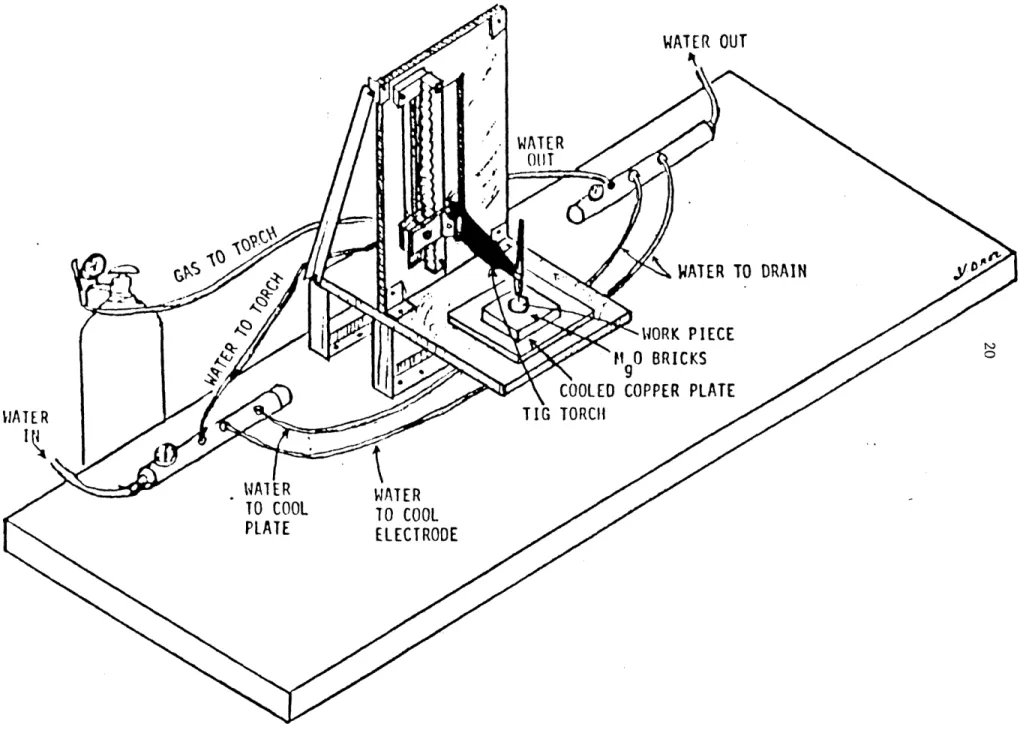
The experimental station consists of a stationary rig, as shown in Figure 4, designed to allow easy modifications and convenient hook-up.

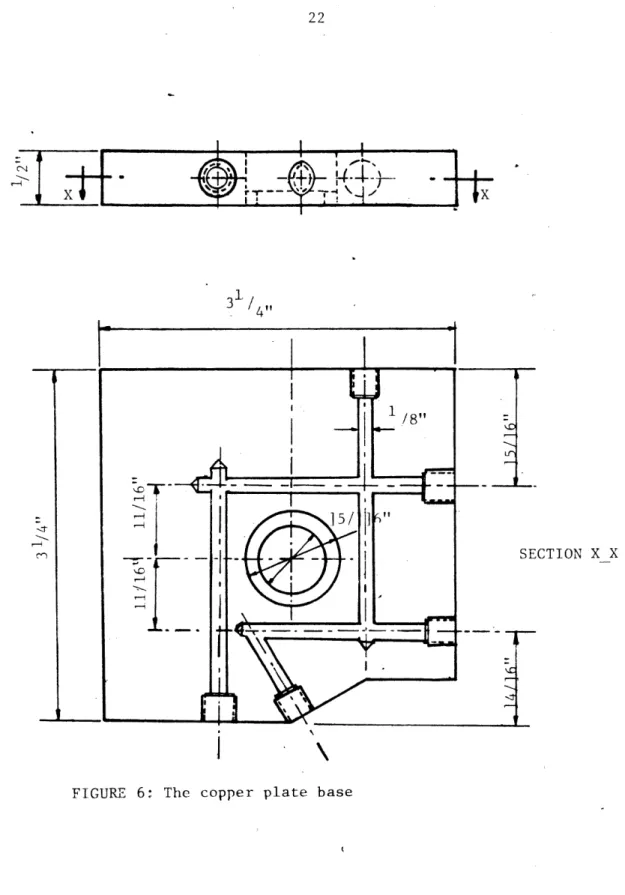
Mild steel, circular workpieces of three different thickness plates of the same diameter (22 mm), as shown in Figure 5, were silver-soldered into the copper base to reduce the contact resistance. The copper base plate (Figure 6) has an approximately symmetric cooling passage and provides the cooling in order the workpiece to be at steady state for the range of heat inputs from the arc.

A GTAW torch (Airco heliweld h20-c) was used in conjuction with 2/32" diameter 2% thoriated Tungsten electrode surrounded by a 3/8" diameter alumina nozzle, through which argon, the shielding gas, was supplied at a flow rate of about 18 cubic feet per hour.

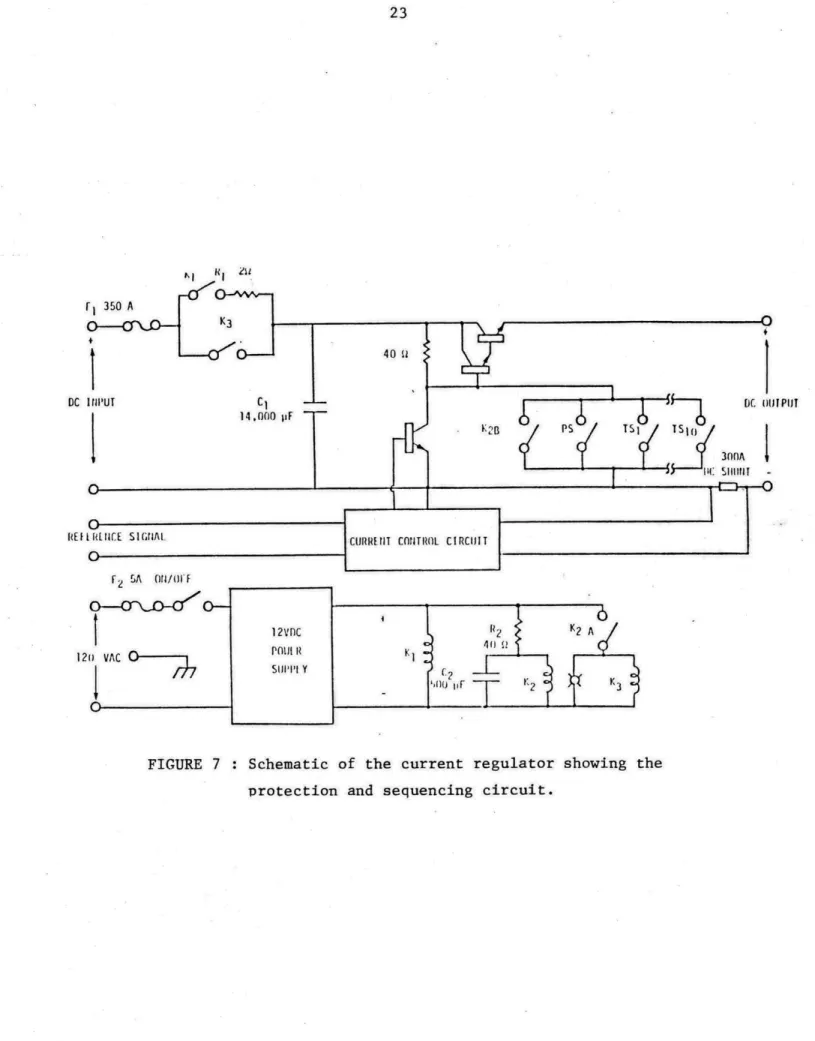
The welding power supply is a 3-phase rectified supply (AircoCV-450) capable of supplying a maximum current of 450 amperes at 38 Volts, with the current level options of 450 and 300 amperes. A shunt with output of 50 mV at 200 amperes was used to measure the current. The voltage between the tip electrode (cathode) and the workpiece (anode) was also measured.

This power supply was used in combination with a transistorized current controller to control the current passing through the arc. A schematic is

shown in Figure 7 and a more detailed description can be found in [101. An external reference signal from 0 to 10 Volts full scale provided by a Krohn-Hite Model 5200A signal generator was used to specify the output current value

from 0 to 300 amperes. The current regulator was designed with the control measurements on the cathode side, since the anode is usually grounded. The cathode (electrode) operates at a negative voltage relative to ground.

qw

WATER OUT

WATER TO DRAIN

WORK

PIECE

I

BRICKS

COOLED COPPER PLATE

TORCH

WATER

TO

COOL

ELECTRODE

FIGURE

4:

OVERALL VIEW OF ARC WELDING EXPERIMENTAL SET-UP

w

1

9

₀

_S

₀

WATER

I {

TO COOL

PLATE

21 7/8' A. workpiece:7/8"*7/32" 7/8" B.workpiece:7/8"*7/24" 7 /F" C.workpiecei: 7/8"*7/]6"

FIGURE 5: The workpieces tested

I

22

3 4

SECTION X X

FIGURE 6: The copper plate base

23 r 350 A K3 40

1

REFICE SIG URAL CURRcIT Cth TROL CIRC uIT

F iA aqn/01F 4 O-2VDC R2 K2 A 120 1VAC O01 114 I _WO> 0 F 112 K3_

FIGURE 7 :Schematic of the current regulator showing the protection and sequencing circuit.

24

A computer based data acquisition system called UnkelScope{ M.I.T.,19831 was used to measure, display and store the data from arc current, voltage, temperatures and power input. This system was developed for the M.I.T

Department of Mechanical Engineering Undergraduate Laboratory by professor W. Unkel. It is a software data-acquisition package, implemented on a Digital

Equipment Corporation (DEC) LSI 11/03 based system operating under RT-11SJ. The analog to the digital converter on UnkelScope was an ADAC Corporation 12 bit converter with programmable gain to give full scale ranges of + 10

Volts,+5 Volts,+2 Volts and +1 volts. A hardware clock board manufactured by Data Translation was used to provide synchronization of the data taking

process. A DEC RX01 floppy disk drive system was used for mass storage. The CRT display terminal was a DEC VT125,while the hardcopy terminal was a DEC LA50.

3.2 EXPERIMENTS AND RESULTS ON THE ARC V-I CHARACTERISTICS

The product V-I (voltage times current) determines the instanteneous power from the arc, part of which is transferred as a heat input to the

workpiece. It is therefore necessary, to establish the precise relation

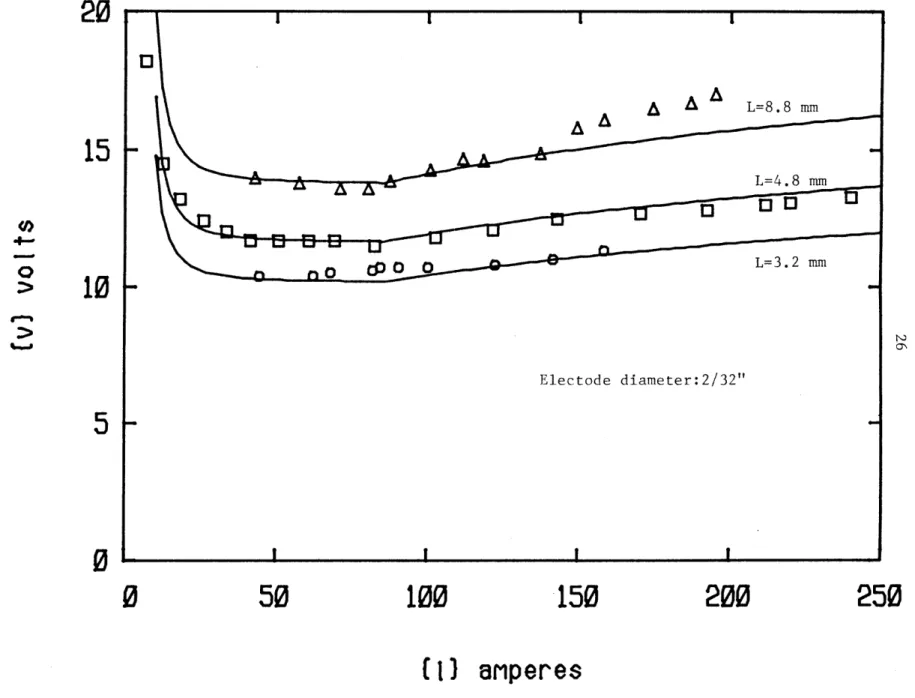
between arc voltage and arc current. In this work V-I measurements were taken for D.C. arcs, but data for A.C. arcs can be found in [11]. The current

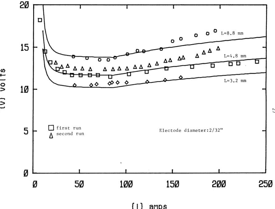
signal from the 300A shunt and arc voltage readings from the electrode were measured using an amplifier and attenuator, respectively, and recorded by the data acquisition system. A strong dependance of the V-I curve on the arc length was expected, so measurements were taken for three different arc lengths: L= 3.2 ,4.8 ,and 8.8 mm . A non-Ohmic behaviour (see Figure 8) was observed due to the strong dependance of electric conductivity on the temperature. As the current increases the emitted power is increased, the

25

temperature of the plasma jet also increases and therefore the electric conductivity increases, so the voltage remains approximately constant depending only on arc length.

An empirical relationship was found to correlate very well the experimental data in the two regions, as:

0.3 -2.~42

V=7.20-L .exp{98.3-I-2.42

when the arc current is in the region from 0 to 85 amperes,and

V=3.70-LO.3 0.15 (2)

when the arc current is in the region from 85 to 250 amperes, and with L in cm.

The solid lines in Figure 8 represent values given by the above equations (1) and (2). These expressions can be used only for argon arcs of

approximately commercial purity, since it has been found experimentally that for nitrogen, for example, the voltage drop can be as high as three times the values predicted by the above expressions.

The overall voltage drop measured is the sum of the voltage drop in the vicinity of the anode, the drop in the so called positive column, and the drop which occurs next to the cathode. Electrons are emitted thermionically from

the cathode, passing through a potential drop in the immediate vicinity of the cathode before entering a region of low potential gradient, known as the positive column which extends over most of the arc length. At the anode another potential drop occurs, before the electrons enter the anode over a small area the anode spot. In low-current arcs the potential gradient of the positive column is uniform, but in high current arcs the positive column is divided into two parts of different potential gradients. In the positive column, being in equilibrium, the electrons colliding with the gas molecules and raise the gas to a high temperature, estimated at about 5000 K. At this

20

A

AA

15

10

5

0

'

0

50

100

150

200

250

(1)

ariperes

20

O

O

o 0

15

A

10

5Electode

0

0

50

100

150

200

250

(1)

amps

28

temperature some of the gas is ionized providing a positive ion current which heats the cathode, but the arc current is largerly carried by the electrons, since although positive ions and electrons exist in approximately equal

numbers in the arc column, the mobility of electrons is much greater than that of ions.

The final value of the total voltage drop depends, also, on the formed weld pool. For a pool with a depressed top surface the effective arc length is increased and an increase in voltage should be expected. This is indicated with experimental data plotted in Figure 9 for arc length 4.8 mm. The

measurements shown by a triangle were taken in a second run after a pool had been formed in the first run (squares) and as expected has a higher voltage drop because of the larger length.

3.3 EXPERIMENTS AND RESULTS ON ARC EFFICIENCY

The energy transfer to the plates is composed primarily of the electron energy and convective heat transfer with the convection part increasing as the arc current increases, but remaining two to three times less than the electron energy transfer.

The power generated in the arc is not all transferred to the workpiece, and an arc efficiency can be defined as the heat used to melt and heat up the workpiece divided by the total emitted power by the torch. The power not transmitted to the workpiece is dissipated by radiation from the arc or is convected away by the flowing gas or is used to heat up the cathode and subsequently tranferred to the torch cooling water. According to our measurements the heat absorbed by the water cooling the electrode is very small. Even with very low cooling rate very small temperature rise was measured and therefore the losses consist mainly of the radiation from the

29

luminous gas and the part that is convected away by the gas. It is rather difficult to evaluate analytically or experimentally these losses, and in the literature there is a large discrepancy of data. Results range from an

efficiency as low as 40% to as high 90% (Wilkinson and Milner,1960, [12]) have been reported. It is therefore important to measure the heat absorbed by the workpiece. With our experimental set up, in steady state, it is expected that

the heat incident on the pool surface will be equal to the heat gained by the cooling water in the copper base plate, since the heat losses from the copper surface are negligible. Thus, the mass flow rate of cooling water, m, and the water temperature rise AT are measured and the heat delivered to the workpiece evaluated as

Q = m-c -AT (3) p

where c =4,187 j/kg, is the specific heat of water.

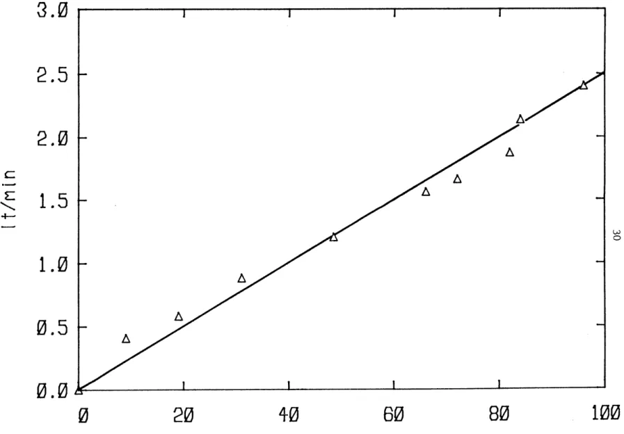
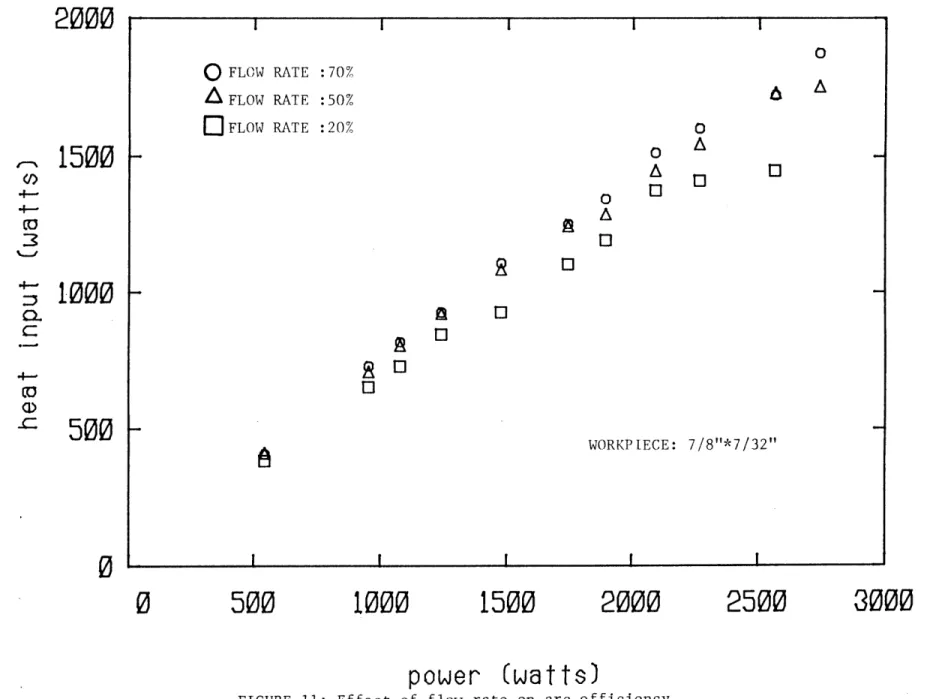
To measure the flow rate of water a rotometer was used, operating at different rates as percentage of the total rate at 100%. At the pressure of 30 psi the volume flow rate was 2.5 lt/min, and the calibration curve is shown in Figure 10. To examine how the different cooling rates could change the evaluated arc efficiency, measurements were taken for 70%,50%and 20% flow rates. As shown

in Figure 11 for 70% and 50%, no change in the heat input was observed,but in the case of low cooling rate (20%), the measured heat was found to be lower, which should be expected since the overall temperature level of the system

(workpiece plus copper plate) was higher and, therefore, the losses from the copper surface start to become important.

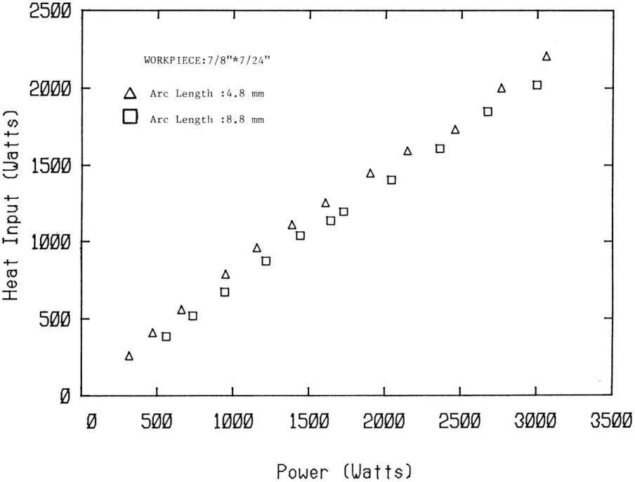
The effect of arc length on the arc efficiency was studied next, by taking measurements at two different arc lengths, L=4.8 mm and L=8.8 mm. As shown in Figure 12 in the case of the long arc the losses are larger and this result agrees with the results reported by other investigators. R.C. Eberhart

W

3.0

2.5

2.0

1.5

1.0

0.5

0.0

0

20

40

60

0

100

80

FIGURE 10: Calibration of flow meter

c:

W W W W

2000

o

A

0

0

0

A

El

DA

01

0

1500

1000

500

0

1000

1500

2000

power (watts)

FIGURE 11: Effect of flow rate on arc efficiency

0

A

6

D

0

500

2500

3000

I

I

I

I

I

W

W

W

W

2500

2000

Al

A

EJ

AU

AU

A6

500

1000

Power (Uatts)

FIGURE 12 :Effect of arc length on arc efficiency WORKPIECE:7/8"*7/24"

LA

0D

:3

A

1500

1000

U

0

A

U

11

Ul

A6

El

r-500

0

0

1500

2000

2500

3000

3500

I

I

I

j

j

j

j

i

j

I

I

I

I

I

I

33

et al [14] have found that the efficiency n is independent of current and depends on the arc length L as :

f = 0.75/LO-13 (L in cm) (4) for currents higher than 200 amperes.

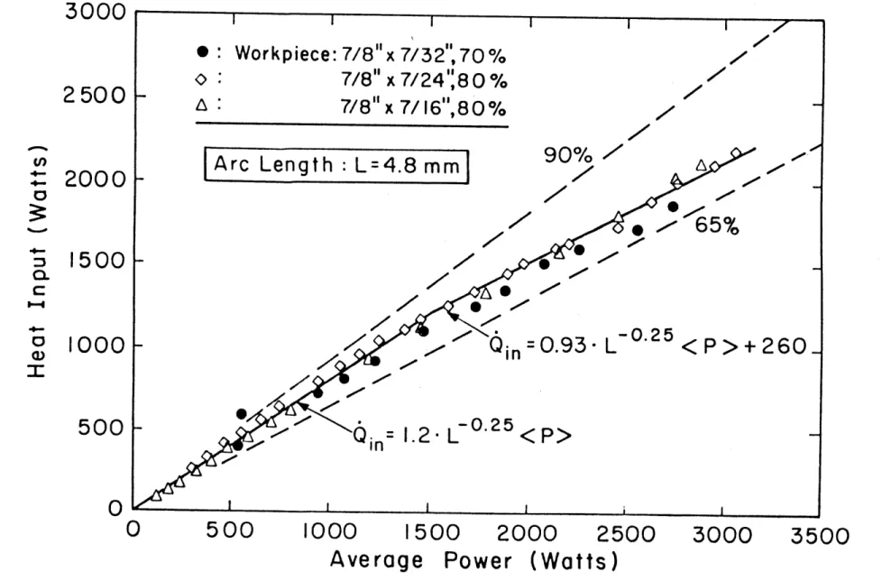
Our results for the three different workpieces indicate that for low current the arc efficiency is, indeed, independent on current, but for higher current values the efficiency decreases as the current increases, and that the dependance on arc length is stronger than that given by [14]. No dependance, however, on the thickness of the workpiece,as it was found by [11] was

observed but a rather universal curve for the heat input was obtained depending on the arc length only. The "knee" behaviour for the Q-P curve shown in the Figure 13 observed at, approximately, 1.5 kwatts of emitted power, is explained from the fact that above this critical power a puddle has formed in the metal and the depression in the surface affects the heat input. In addition, the radiative losses become more pronounced for higner current values.

For computational purposes an empirical fitting formula for the two different regions is obtained for the heat input obtained from the

experimental data:

n = 1.20/L0.25 (5)

when the average power from the jet is not exceeded the 1500 watts, and as

0-93/LO.25 +260/{P} (6)

when the incident power is in the range of 1500 watts to 3500 watts.

Finally, experiments were conducted to determine the arc efficiency for the promising technique of current pulsing. Although, the data are not

U U l

W

3000

Workpiece: 7/8"

_x

_7/32",70

_%

7/8"

x

7/24',80

%

2500 -

_207/8'

x

7/16",80%

Arc Length

L=4.8

mm

90%

2

-0000

65//65%

1500 -/

0..

1000-

Oin

0.93- L

<

P>+260

500-

₆

_-o.25

0

0

500

1000

1500

2000

2500

3000

3500

Average Power (Watts)

S

0

0

0

3000

1

1

2500

o

4& Pulsed current

xx

2000

0H--1500

o

x

10000.6W

500

Note:Numbers indicate ratio of current amplitude/average current

0

0

500

1000

1500

2000

2500

3000

3500

(P)

UATTS

36

at high heat inputs and for large current pulsing the effective heat input is slightly larger as it is compared with the D.C. case. For smaller current pulsing no difference in the results was observed. It is expected that in the case of thinner workpieces the small difference observed here will be wre pronounced.

To determine analytically the arc efficiency it is a very complicated problem, since the heat that, finally, is delivered to the workpiece is composed of various components, as follows:

QQ +Q +Q + Q r(7)

$I e c r

where the first two terms on the rhs denote the contribution from the electrons as Q =I-$, where $ is the work function, depending on the anode material,for copper, for example, is 4.3 eV, and

0Q

contribution is:

QeT - I-(O+V a+3-k-T/(2-e)) (8)

To calculate the radiation energy transfer Q, the diameter of the luminous region of the arc, the absorption coefficient of the anode and the emission coeffic ient of the gas must all be known. In general, Qr is a small fraction (approximately one tenth) of the convective heat Sc. The convective part c, for low current is a small fraction of the total heat to the anode, but as the current increases Qc increases more rapidly than eT' which increases almost linearly with current, since Va does not change much.

One way to represent the convective heat transfer is to employ an effective heat transfer coefficient h, as

37

Q =h-AT-Area (9)

C

where h can be evaluated for axisymmetric stagnation type flow,as h=0.76-(y-c /k) -(U-d/v)0.5 (10)

p

where d is the jet diameter. Then, h can be evaluated to be from 1000 (200) to 1500 (300) W/m 2K (Btu/hrft2 ).

It is much more difficult to evaluate the temperature distribution and therefore to obtain the temperature potential AT. However, it is reported by Converti [101 that AT is a weak function of current. The jet velocity has been found to vary linearly with current, and therefore:

Q will be proportional to I12 e

whereas, Q ewill be proportional to I.

For low current values and arc lengths less than 6 mm it has been found [14] that Qc is always less than 25% of the convective flux and therefore the total heat input will increase roughly linearly with current.

3.4 TEMPERATURE MEASUREMENTS

Thermocouples were spot welded on the workpiece surface at various

locations and temperatures were recorded using the data acquisition system and an Omega digital thermocouple thermometer.

The centerline backside temperature is expected to be a good indication of the size of the weld pool and therefore a good measure for comparison with the values predicted by the model; this temperature was measured for the three workpieces. For the thin workpiece (7/8"-7/32") and the medium thickness

workpiece (7/8"-7/2411") the topside temperature at a distance 7.4 mm from the centerline was measured. The thermocouples were shielded to eliminate the effect of the very strong radiation from the arc, which otherwise could alter significantly the thermocouple signal. For the third workpiece the backside

38

temperature at a location 5.0 mm from the centerline was also measured; a copper/constantan thermocouple was used, since the range of this temperature was not expected to exceed 700 degrees Celcius.

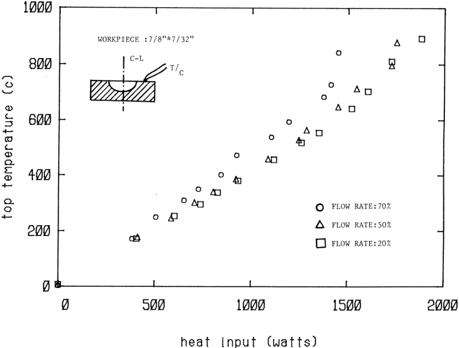
To check the effect that the water cooling rate could have on the temperature level of the system, experiments were conducted with different cooling rates, 70%,50% and 20% of the maximum flow rate. As shown in the Figure 15 the cooling rate has no effect in the measured temperature, except

in the case of very low flow rate, for which a strongly assymetric cooling results. In such cases the water temperature rise is more than 20 degrees C

for relatively high heat inputs.

All the measurements were being taken after waiting at least one minute in order for the system to have enough time to equilibrate at steady state. The time constant, as it can be shown either from the transient measurements or from analytical calculations was less than 15 seconds.

The arc length is also an important factor upon which the temperature of the system depends. In Figure 16 the centerline temperature for the second (medium thickness) workpiece is plotted against the effective heat input, the heat delivered to the cooling water. In the case of the long arc a large

temperature drop was recorded for emitted power above 1 kw, after the puddle is formed. Such a temperature drop should be expected, although probably, not so dramatically, since the anode spot of the heat input is expected to

increase with the arc length and therefore the heat input is not as focused as in the case of shorter arc lengths.

In the next Figure 17 the centerline back temperature is plotted as a function of the effective heat input for the three plates. The centerline back temperature is very sensitive to the heat input with the slope dT/dQ increasing as the penetration increased. Near full penetration the changes

1000

A

800

-

600

0

(E 4-000

0-

0

200

CI

0

0

500

1000

1500

2000

heat

input (watts)

LJ

0

I

1600

1+00

1200

1000

800

600

400

200

0

aJ

EAA

500

heat input (watts)

FIGURE 16: Centerline back temuerature for different arc lengths CD C--cc) T/C

A

A

A

A

A

A

A

A

A

A

rt

1

a0

a0

0

a0

0

1000

1500

2000

2500

I

I

I

I

a I C-L T melt

1600

1100

1200

1000

800

600

1-00

200

A

A

O

O A

₀

500

heat input

(watts)

FIGURE 17: Centerline back temperature for different worknieces

A

A

A

0'

A

A

A

A

A

A

A

0

0

01

0l

01

E0

0

1000

1500

2000

2500

.

.

.

A

EM6

_I

_I

42

are extremly rapid. For the thick workpiece for which full penetration is expected to occur only above 4 kw effective heat the centerline back temperature varies almost linearly with the heat input with a change of 50 degrees C for 500 watts. For the medium thickness workpiece the corresponding

change is 250 degrees C per 500 watts. It is seen that a very detailed recording of the centerline temperature was obtained for the second workpiece with a chromel/alumel thermocouple responding up to nearly the melting

temperature. The maximum temperature recorded just before the full

penetration was 1337 degrees C, the melting temperature of mild steel being at 1347 degrees C. Unfortunately, with the thin workpiece the constant/copper thermocouple used did not respond above 500 degrees C and the data are very limited in this case. Finally the experiments for the thick workpieces were repeated three times to ensure that the measurements taken were correct since their magnitude was rather low. In Figure 18 the top temperature for the small and medium thickness workpieces are presented with the thinner workpiece

experiencing higher temperature. That the effect of the strong radiation from the arc was completely eliminated using insulated chromel/alumel thermocouples could easily be observed during the experiment, since when a signal from the emitted radiation heat is picked up the thermometer intications are very unsteady, but no such fluctuation were observed.

For the thick workpiece the back temperature was measured instead of the top temperature at a distance 5.0 mm from the center, as shown in Figure 19. It is seen that the slope dT/dO is not larger that the slope of the centerline back temperature, which was also low as it was compared with the thinner

workpieces. The linear response at small values of heat input is expected, since at low heat input pure conduction occurs with no puddle formed yet and also the losses from the back surface due to radiation and natural convection (hot plate facing downwards) are small.

W V

A

0

A

A

'A

A

A

A

01

01

01

500

0l

0

0

heat input(Watts)

FIGURE 18 :Too side temoerature versus effective heat input

1000

800

A

A

A

600

400

A

A

A

01

0

E0

0

01

200

0I

0

2500

1000

1500

2000

I

I

I

I

I

WORKPIECE:7/8"*7/16"

400

350

300

250

200

150

100

50

0

A

A

A

A

A

A

o

C-ci

A

A

1000

1500

2000

500

2500

heat [nput (watts)

A

FIGURE 19:Back temperature versus effective heat input

A

A

A

A

A

A

A A

0

I

I

I

I

I

I

k

v

0

1000

800

500

1000

₁

₅₀₀

2000

2500

(P)

UATTS

FIGURE 20 *Effect of current pulsing on the centerline back temperature

Frequency:100 kHz WORKPIECE:7/8"*7/16" Solid Line:D.C. Data

..-J

<

wt

Q_

.J

600

/+00

200 k

0

3000

46

To examine the effect of the current pulsing on the temperature level of the system the centerline back temperature was measured for the thick

workpiece and plotted in Figure 20, where a comparison is being made with the case of D.C. For ratios of current amplitude over average current larger than unity slightly higher temperatures were measured, but no difference was

observed for this ratio being less than one. It is expected that in the case of thinner workpieces a different respond would occur.

3.5 VELOCITY MEASUREMENTS

The difficulties involved in the measurement of velocities within a puddle of high temperature melt are self evident. In addition to this the very small dimensions of the weld pool make this task almost impossible. On the other hand, it is very important for heat transfer calculations to

establish a realistic order of magnitude for the Reynolds number inside the pool and furthermore the velocity field.

To determine the direction of the flow inside the pool a tungsten colored node was inserted into the hole drilled into the workpiece of dimensions

7/8"- 7/24" at about 8 mm deep from the side and 1.5 mm from the top at a

location, where a molten steel puddle was expected to be formed. After the experiment was finished the workpiece was cut at exactly this position ,but the tungsten node was not there, apparently moved to another place by the

flow.

This attempt along with other investigators attempts to estimate the velocity of the interior flow show that direct measurements of the flow in the real system is a rather unsolved problem, at least at the present time.

There have been reported, however, indirect measurements of the pool surface velocity in the real system, or in similar systems, by taking a time

47

exposure photographs of a small bead of material (glass, for example) as it was swept across the surface. This, of course, gives no indication of the

flow underneath, which can even have the opposite direction, and on the other hand the reported values of surface velocity for almost the same conditions with GTAW vary from a few millimiters per second to one meter per second. It has been reported by Woods and Milner working with pools of mercury that the observed intensity of motion was varying as the square of the arc current, increasing also, with the melting point for different materials.

Mercury at room temperature has a viscosity of 0.00161 Nt-s/m 2, close to that of molten steel and so the room temperature mercury pool may be expected to show similar behaviour to that of large high temperature melts. However, to keep in the same conditions in the simulation experiments as in the real case is very difficult. For instance, a crust of mercury oxide forms on the pool surface, and this layer likely alters the surface tension characteristics of the melt. For the mercury, thermally induced motion can be large, whereas

for the real system this effect is almost negligible. This problem encountered by Sadoway et al [15], who conducted experiments with molten

salts, a binary mixture of KCl and LiCl, using a Laser doppler anemometer to measure velocities in this transparent materal. The problem was that the flow

induced was caused not by electromagnetic forces from the applied current through the metals, but by the dominant buoancy forces.

To keep the same real welding conditions in the simulation experiments a complete set of simulation criteria, as determined from the equation of motion and the electromagnetic field, must be met.

If the effect of velocity of the metal on the magnetic field is neglected (a reasonable assumption since the magnetic Reynolds number for welding

conditions of steel plates is much less than unity) a complete set of similarity parameters for the steady state is as follows:

48

11 =p-U-12/ 0/ 1 2= inertia force /em force 2

2 =Pm-U-1/00 2 =viscous force/em force I3 p-g3l 2 =gravity force/em force

where y 0 is the magnetic permeability, pm the dynamic viscosity of the melt and

1 is a characteristic length. To keep only the two parameters ,2

Hq

11 = constant, therefore Iq /I2=5

R2 = constant, therefore U 1 /U2 1 2=7

The above relations indicate that 100 amperes of arc current for the real system correspond to only 20 amperes to the Hg system, but still it is not

sure if the mercury with a boiling point of 357 degrees C will not evaporate. Gallium with boiling point of 2205 degrees is suitable for this use, since all

its other properties are similar but it has a very high cost.

3.6 CROSS WELD SECTIONS

After each experiment, the molten metal was removed from the weld pool by suddenly applying a very high water cooling rate, as the arc was turned off. The rapid cooling prevented the melt from binding with the solid material so

the solidified content of the pool could be removed with a screwdriver. After the pool material was removed the workpiece was cut across the centerline and was grounded and polished.

The experiment with the thick workpiece was repeated three times, so three different weld cross sections were produced under slightly different welding conditions. The very shallow puddle, shown in Figure 21.a, was produced by applying a rather low d.c. current and very high cooling rate, whereas the very uniform parabolic melting boundary shown in Figure 22.a was

49

IrT-I-F-

IITTTvI

I-n

IFImTFFFFFFF

OrwrrrFF

FIGURE 21 a:Shallow puddle for workpiece 7/8"*7/16"

ii

21

i

pntai f

1111-oi11

118"*7321

50

iii

liii 1111111111111

FIGURE 22 a Parabolic boundary

51

produced by applying current up to 240 amperes and 80% cooling rate. To demonstrate the effect of the concetrated impurities three small holes were symmetrically drilled from one side of the disk workpiece and a small amount of green powder of Cr203 was put in the holes as well as in the pool surface bounded in place by using a paint as an organic binder. The effect of Cr2 0 3is

twofold. First it changes the surface tension characteristics of the molten steel and therefore affects the intensity of the motion with more heat flowing outwards to the cold edge so that a more shallow puddle is produced. Second, it changes the wetting angle and this affects again the radial surface flow. The resulted weld pool is shown in Figure 22.b.

The two other workpieces were fully penetrated the first (thin), Figure 21.b, at arc current of 190 amperes and the second at 210 amperes.

3.7 MEASUREMENT OF T

An attempt was made to measure the maximum temperature in the weld pool expected at the centerline of the pool just underneath the electrode tip. A CCD array was used purchased from E.G.and G. with 256 elements. The CCD array was focused on the centerline of the pool to pick up the radiation emitted from the very hot pool surface. Although a diaphragm and an infrared filter was used to reduce the light intensity from the arc its effect were not completely eliminated and the final recorded signal was not sure if it caused by the radiation emitted by the high temperature pool surface.

More work is needed to first calibrate the CCD array according to a standard temperature scale in the high range from 1500 degrees and above. By selecting the proper infrared filter since the spectral scan of the hottest part of the argon shows strong peaks in the red and infrared region, it should be possible to measure the maximum temperature of the pool, the importance of

52

which is self evident, since it is expected to be a very precise indication of the weld pool size and one of the variables to be sensed in the real contol applications when no access in the backside of the plates for the measurement of the temperature is possible.

3.8 SUMMARY

To summarize, in this chapter the experimental apparatus was described first and data on the arc voltage-arc current relation, on the arc efficiency and on the surface temperature were then presented. A universal curve was found to correlate the experimental data for the arc efficiency with lower efficiency measured at higher current values. The effect of impurities was also studied and the addition of Cr203 on the molten steel was found to alter dramatically the weld pool shape.

53

CHAPTER FOUR THEORETICAL ANALYSIS

4.1 INTRODUCTION

Within the context of control systems for weld geometry it is important to understand and develop computationally simple models to predict the puddle size. The model must be capable of predicting the effect of a variety of parameters, such as the heat input, the welding torch speed, the arc length, and the impurities in the pool.

Since the motion in the pool cannot be ignored in the heat transfer calculations it is essential to investigate the possible mechanisms, which give rise to motion. Stirring type fluid motion in the puddle can be caused by several such mechanisms including electromagnetic stirring forces, surface tension forces resulting from the nonuniform surface temperature, shear and normal forces exerted on the puddle surface by the plasma flow and the buoyancy forces resulting from the large temperature gradients within the pool. All these forces, which may reinforce each other or conflict with each other are responsible for the directionality of the heat flow in the pool as compared with what would be expected from pure conduction only. The overall effect is the formation of very shallow weld puddles when the fluid and heat flow radially outwards in the pool surface or deep puddles when the main motion is radially inwards.

If the heating was from a point source in the case of a thick block of metal and there was no interior motion the melting boundary would be

hemispherical as it is predicted by the conduction heat transfer theory. In the real case the shape of the pool is not known and it is a very difficult

54

problem to determine both the precise shape and the size (dimensions) of the pool. The approach adopted in this work is to solve the coupled fluid flow and heat flow field with a free boundary (melting interface) by postulating the shape of the boundary to be generally consistent with the puddle shapes observed from our experimental data and the results of other investigators and

then determining from the model the size of the pool for a specified set of conditions. Results for a two shape parameter model have been completed and work on a three shape parameter model have been started.

The solution technique is to split the problem into three regions (a) the arc (b) the solid material and (c) the molten metal region and then solve iteratively since the physical phenomena occuring in these three regions are coupled.

A numerical model for a GTA arc has been developed by Converti [10] and in this work only experiments were conducted to determine the arc-voltage relation and the arc efficiency. The mode of heat transfer through the solid material is conduction, a well posed problem with the outer edge of the plate at prescribed temperature. In the liquid region the enhanced heat transfer is taken into account by determining first the motion of the melt and then apply the principles of heat convection. After the solution in the convection and conduction sides have been obtained, the heat fluxes at the solid/liquid boundary are tested to see if they match. If the results for the convection side and conduction side do not match a new boundary is specified (by its depth and width) and the solution procedure repeated.

55

4.2 CONDUCTION IN THE SOLID

For the stationary configuration used in this work the full problem for the weld puddle formed is displayed in Figure 23.a. Axisymmetry allows reduction to the half width (two dimensional) geometry as shown in Figure 23.b. The outer face of the workpiece is in contact with the cooled copper base which is kept at the coolant temperature 10 0 C. The lower and upper surface are assumed to radiate as a grey body with a specified emissivity. The effect of natural convection from the surfaces was included using a temperature dependent heat transfer coefficient. To show the importance of the heat losses, adiabatic bottom and top surfaces have also been examined The conduction problem is linear when the boundary conditions are adiabatic, but radiation and natural convection introduce nonlinearities which can increase the computational time by a factor of two.

4.2.1 FINITE ELEMENT MESH EMPLOYED

The conduction solution was obtained with a general purpose heat transfer finite element code ADINAT [211, developed at M.I.T. For steady state various finite element meshes were tested before the final mesh selection.

Optimization requires that with a minimum number _{of nodes and elements a good} agreement for the computed heat fluxes at the nodes common to more than one element to be obtained. In the meshes shown in Figures 24 through 27, 24 isoparametric elements with 98 nodes were used. The size of the elements is changed automaticaly as the mesh is deformed to capture any shape of the weld pool. In the first mesh, shown in Figure 24, the weld pool boundary is a parabola, in comparison to Figure 25 where the pool shape is simulated by a combination of an ellipse in the uppermost element and a parabola bound the

56

ele ctrod

ano

FIGURE 23 a:Demonstration of axisymmetric conditi

FIGURE 23 b:Reduction to half width geometry

-

w

a

th(Th

IT

d

c

10

8

83

0

2

4

6

8

10

12

14

16

18

20