HAL Id: hal-00328530
https://hal.archives-ouvertes.fr/hal-00328530
Submitted on 18 Sep 2007
HAL is a multi-disciplinary open access
archive for the deposit and dissemination of
sci-entific research documents, whether they are
pub-lished or not. The documents may come from
teaching and research institutions in France or
abroad, or from public or private research centers.
L’archive ouverte pluridisciplinaire HAL, est
destinée au dépôt et à la diffusion de documents
scientifiques de niveau recherche, publiés ou non,
émanant des établissements d’enseignement et de
recherche français ou étrangers, des laboratoires
publics ou privés.
constituent transport in deep convection
M. C. Barth, S.-W. Kim, Chen Wang, K. E. Pickering, L. E. Ott, G.
Stenchikov, M. Leriche, S. Cautenet, J.-P. Pinty, Christelle Barthe, et al.
To cite this version:
M. C. Barth, S.-W. Kim, Chen Wang, K. E. Pickering, L. E. Ott, et al.. Cloud-scale model
intercom-parison of chemical constituent transport in deep convection. Atmospheric Chemistry and Physics,
European Geosciences Union, 2007, 7 (18), pp.4731. �hal-00328530�
www.atmos-chem-phys.net/7/4709/2007/ © Author(s) 2007. This work is licensed under a Creative Commons License.
Chemistry
and Physics
Cloud-scale model intercomparison of chemical constituent
transport in deep convection
M. C. Barth1, S.-W. Kim1,*, C. Wang2, K. E. Pickering3,**, L. E. Ott3,**, G. Stenchikov4, M. Leriche5,***, S. Cautenet5, J.-P. Pinty6, Ch. Barthe6, C. Mari6, J. H. Helsdon7, R. D. Farley7, A. M. Fridlind8,****, A. S. Ackerman8,****,
V. Spiridonov9, and B. Telenta10
1National Center for Atmospheric Research, Boulder, CO, USA
2Massachusetts Institute of Technology, Cambridge, MA, USA
3University of Maryland, College Park, MD, USA
4Rutgers University, New Brunswick, NJ, USA
5CNRS/University Blaise-Pascal, Clermont-Ferrand, France
6CNRS/Paul Sabatier University, Toulouse, France
7South Dakota School of Mines and Technology, Rapid City, SD, USA
8NASA-Ames Research Center, Moffett Field, CA, USA
9Hydrometeorological Institute, Skopje, Macedonia
10SENES Consultant Ltd., Toronto, Canada
*now at: ESRL/CSD and CIRES, University of Colorado, Boulder, CO, USA
**now at: NASA-Goddard Space Flight Center, Greenbelt, MD, USA
***now at: CNRS/Paul Sabatier University, Toulouse, France
****now at: NASA-GISS, New York City, NY, USA
Received: 14 May 2007 – Published in Atmos. Chem. Phys. Discuss.: 8 June 2007
Revised: 6 September 2007 – Accepted: 8 September 2007 – Published: 18 September 2007
Abstract. Transport and scavenging of chemical con-stituents in deep convection is important to understanding the composition of the troposphere and therefore chemistry-climate and air quality issues. High resolution cloud chem-istry models have been shown to represent convective pro-cessing of trace gases quite well. To improve the represen-tation of sub-grid convective transport and wet deposition in large-scale models, general characteristics, such as species mass flux, from the high resolution cloud chemistry mod-els can be used. However, it is important to understand how these models behave when simulating the same storm. The intercomparison described here examines transport of six
species. CO and O3, which are primarily transported, show
good agreement among models and compare well with
obser-vations. Models that included lightning production of NOx
reasonably predict NOxmixing ratios in the anvil compared
with observations, but the NOxvariability is much larger than
that seen for CO and O3. Predicted anvil mixing ratios of the
soluble species, HNO3, H2O2, and CH2O, exhibit significant
differences among models, attributed to different schemes in these models of cloud processing including the role of the Correspondence to: M. C. Barth
(barthm@ucar.edu)
ice phase, the impact of cloud-modified photolysis rates on the chemistry, and the representation of the species chemical reactivity. The lack of measurements of these species in the convective outflow region does not allow us to evaluate the model results with observations.
1 Introduction
Convective processing of trace gas species is an important means of moving chemical constituents rapidly between the boundary layer and free troposphere, and is also an effec-tive way of cleansing the atmosphere through wet deposi-tion. Because of these two processes, the effect of convec-tion on chemical species is critical to our understanding of chemistry-climate studies, air quality studies, and the effects of acidic precipitation on the earth’s surface.
In large-scale models convective parameterizations have been developed primarily on the basis of mass and heat fluxes. An intercomparison of several convective parameter-izations used in both global and regional scale models shows that there is significant variability among the parameteriza-tions (Xie et al., 2002; Tost et al., 2006). Lawrence and Rasch (2005) compared tracer transport in deep convection
for plume ensemble and bulk formulations of convective
transport parameterizations. Their results showed
differ-ences in the upper troposphere of up to 25% between the plume ensemble and bulk formulations of convective trans-port for the July monthly mean mixing ratios of decaying, insoluble scalars. At shorter averaging times, the differences between the two formulations are even greater. Clearly there is a need to improve the parameterizations of trace gas trans-port by convection in the global models.
On the other hand, many previous studies using high reso-lution cloud-resolving models (or convective cloud models) have shown that case-specific simulations are able to repre-sent the storm structure and kinematics, such as radar reflec-tivity, wind speed and direction, and outflow heights. Con-vective cloud models coupled with chemistry simulate the re-distribution of passive trace gas species well (e.g. Pickering et al., 1996; Stenchikov et al., 1996; Wang and Prinn, 2000; Skamarock et al., 2000; DeCaria et al., 2000). The cloud-resolving models, when incorporated with reasonably com-prehensive chemistry, can also provide details of cloud pro-cessing of soluble chemical species as well as tropospheric production/destruction of short-lived species including crit-ical hydrogen oxides precursors and aerosols influenced by the existence of convection (e.g. Wang and Chang, 1993b, c; Wang and Crutzen, 1995; Wang and Prinn, 2000; Barth et al., 2001, 2007; Ekman et al., 2004, 2006; DeCaria et al., 2005). Adequate representation of cloud processing of reactive and soluble species in the large scale models is still in demand.
Convective transport and wet deposition of chemical species in large-scale models are sub-grid scale processes and thus have to be implicitly represented by various param-eterizations using grid resolving variables. To improve these parameterizations, the high resolution and process-oriented convective-scale model can be used to obtain general charac-teristics of these sub-grid processes in particular when mul-tiple cloud resolving models are involved. Before gather-ing convective transport characteristics of tracers from mul-tiple cloud resolving model simulations of different storms, it is important to understand how these models behave when simulating the same storm. Results presented here as part of the 6th International Cloud Modeling Workshop (Grabowski, 2006) Case 5 intercomparison provide a means to make an initial comparison of a variety of cloud resolving models cou-pled with chemistry.
The Chemistry Transport by Deep Convection Intercom-parison case was designed to assess the capability of each model to transport different chemical species from the boundary layer to the upper troposphere including the
en-trainment of free tropospheric air. Parameterizations of
lightning-produced NOxare part of the intercomparison
ex-ercise. Carbon monoxide (CO) and ozone (O3) are
com-pared as tracers of transport because the lifetime of the storm (hours) is shorter than the chemical lifetime (days to months)
of these species. Nitrogen oxides (NOx=NO+NO2) are
ex-amined to assess transformation, transport, and NOx
produc-tion by lightning. Nitric acid (HNO3), hydrogen peroxide
(H2O2), and formaldehyde (CH2O) are compared to evaluate
chemical transformation and transport of soluble and reactive species.
2 Description of the case
The 10 July 1996 STERAO (Stratospheric-Tropospheric Ex-periment: Radiation, Aerosols, and Ozone) case was ob-served near the Wyoming-Nebraska-Colorado border. The isolated storm evolved from a multicellular thunderstorm to a quasi-supercell. Observations of the storm were obtained from several platforms including the CSU CHILL radar, the ONERA lightning interferometers, the NOAA WP3D air-craft, and the UND Citation aircraft. These observations are summarized by Dye et al. (2000). Because the 10 July STERAO storm has a comprehensive set of observations and previous model simulations have proven to successfully rep-resent the observed storm (Skamarock et al., 2000, 2003; Barth et al., 2001, 2007), this case is appropriate for inter-comparison of cloud chemistry models.
The simulations performed for the intercomparison mimic those described by Skamarock et al. (2000) and Barth et al. (2001, 2007). The environment was assumed to be homo-geneous, thus a single profile was used for initialization. The initial profiles of the meteorological data were obtained from sonde and aircraft data (Skamarock et al., 2000). To start the convection quickly so that the intercomparison could focus on chemical species transport, the convection was initiated
with 3 warm bubbles (3◦C perturbation) oriented in a NW to
SE line following Skamarock et al. (2000). Their choice of three bubbles was based on obtaining a good representation of the storm structure and evolution (particularly the transi-tion from a multicell storm to a quasi-supercell) with their cloud model. Using the same initiation protocol in each of the participating models will likely produce different storm structures and evolution because of the different methodolo-gies employed in each model. Showing how each model re-sponds to the same initiation is valuable in itself. Simulations were integrated for a 3-h period.
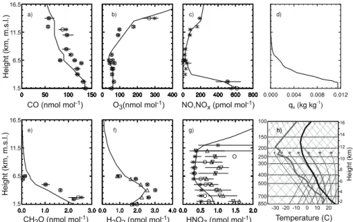
The initial profiles (Fig. 1) of the chemical species are primarily from the aircraft observations obtained outside of cloud. CO is a surface tracer with a surface mixing ratio of
135 nmol mol−1. CO mixing ratios in the free troposphere
range from 90–110 nmol mol−1in the mid-troposphere and
50–90 nmol mol−1in the upper troposphere. O
3mixing
ra-tios are fairly constant with height to about 7 km mean sea
level (m.s.l.), above which O3mixing ratios rapidly increase
into the stratosphere. The initial profile of NOxis based on
NO measurements outside of cloud. NOxmixing ratios are
∼500 pmol mol−1near the surface, but quickly decrease to
values near 50 pmol mol−1 in the mid troposphere. At high
altitudes NOxincreases to 200 pmol mol−1. CH2O and H2O2
-30 -20 -10 0 10 20 Temperature (C) 100 150 200 250 300 400 500 700 850 16 14 12 10 2 4 6 8 Height (km) 16.5 11.5 6.5 1.5 16.5 11.5 6.5 1.5 CO (nmol mol-1) O
3(nmol mol-1) NO,NOx (pmol mol-1)
CH2O (nmol mol-1) H2O2 (nmol mol-1) HNO3 (nmol mol-1)
Height (km, m.s.l.)
Height (km, m.s.l.)
Fig. 1. Initial profiles (black lines) of the chemical species simulated in the case. Circles (average) and asterisks (median) points are from aircraft (UND Citation above 5 km, m.s.l.; NOAA WP3D below 7 km, m.s.l.) observations outside of cloud near the 10 July 1996 storm. In panel (c), the points are observed NO mixing ratios and the line is the NOxprofile used to initialize the models. In (d), qvis water vapor.
On the H2O2profile plot (f), points are for total peroxide measurements except for the triangles which are for 0.85 times the total peroxide.
Circles (average) and asterisks (median) on the HNO3profile plot (g) are from NOymeasurements taken aboard the NASA DC8 during
the SUCCESS field campaign in April–May 1996. Triangles (average) and nablas (median) on the HNO3profile plot (g) are from NOy
measurements taken aboard the NCAR Sabreliner during the ELCHEM field campaign in August 1989. In (h) a skew-T diagram shows the initial thermodynamic state.
combined with values obtained from the literature for high altitudes (Cohan et al., 1999; these initial profiles are in line
with observations reported by Snow et al., 2007). CH2O
decreases from the surface to <200 pmol mol−1in the
mid-troposphere. H2O2 mixing ratios peak near the top of the
boundary layer then rapidly decrease in the mid to upper
tro-posphere. HNO3mixing ratios are based on NOy
measure-ments from the NASA SUCCESS (Jaegl´e et al., 1998) and the NSF ELCHEM (Ridley et al., 1994) field campaigns.
3 Description of the models used in the intercomparison
Eight modeling groups submitted results for comparison. Ta-bles 1 and 2 identify each group and key characteristics of their models. All models were configured to resolve the deep convection with fine scale resolution so that subgrid convec-tive parameterizations were not needed. Although the mod-els described below include a radiation scheme, the radiation parameterization was not activated except for the C. Wang model. The radiation effects on the cloud dynamics should be small for the short (3 h) simulation of deep convection.
3.1 WRF with aqueous chemistry (WRF-AqChem,
M. Barth and S.-W. Kim)
A simple gas and aqueous chemistry scheme has been incor-porated into the Weather Research and Forecasting (WRF) model (Barth et al., 2007). The WRF model solves the con-servative (flux-form), nonhydrostatic compressible equations using a split-explicit time-integration method based on a 3rd order Runge-Kutta scheme (Skamarock et al., 2005; Wicker and Skamarock, 2002). Scalar transport is integrated with the Runge-Kutta scheme using 5th order (horizontal) and 3rd order (vertical) upwind-biased advection operators. Trans-ported scalars include water vapor, cloud water, rain, cloud ice, snow, graupel (or hail), and chemical species. Aerosols are not included in this version of WRF.
The cloud microphysics is described by the single moment (bulk water) approach (Lin et al., 1983). Mass mixing ratios of cloud water, rain, ice, snow, and hail are predicted. Cloud water and ice are monodispersed and rain, snow, and hail have prescribed inverse exponential size distributions. For the simulations performed here, hail hydrometeor character-istics (ρh=900 kg m−3, No=4×10⁴m−4) are used.
The chemistry represents 28 gas-phase and 15 aqueous-phase reactions (Barth et al., 2007) of 15 chemical species:
methane (CH4), CO, O3, hydroxyl radical (OH),
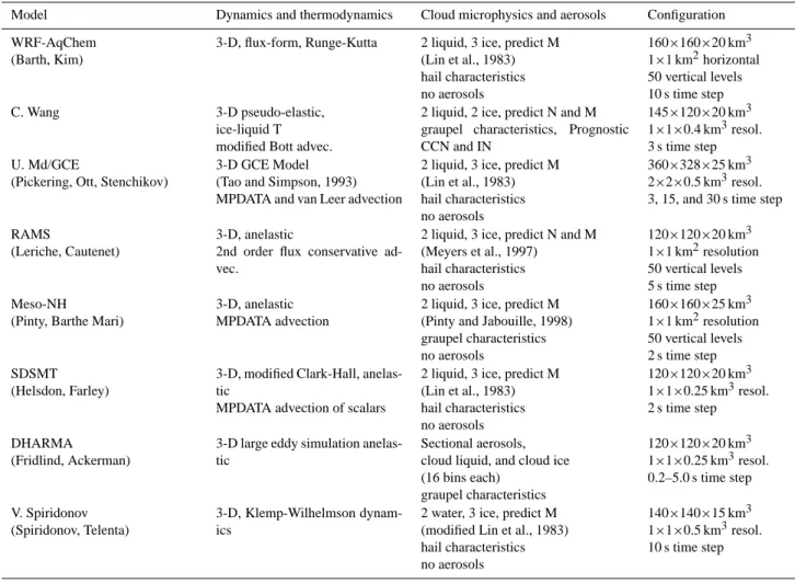
Table 1. Description of the model dynamics, microphysics and configuration used for the simulations.
Model Dynamics and thermodynamics Cloud microphysics and aerosols Configuration WRF-AqChem
(Barth, Kim)
3-D, flux-form, Runge-Kutta 2 liquid, 3 ice, predict M (Lin et al., 1983) hail characteristics no aerosols 160×160×20 km3 1×1 km2horizontal 50 vertical levels 10 s time step C. Wang 3-D pseudo-elastic, ice-liquid T modified Bott advec.
2 liquid, 2 ice, predict N and M graupel characteristics, Prognostic CCN and IN
145×120×20 km3 1×1×0.4 km3resol. 3 s time step U. Md/GCE
(Pickering, Ott, Stenchikov)
3-D GCE Model (Tao and Simpson, 1993) MPDATA and van Leer advection
2 liquid, 3 ice, predict M (Lin et al., 1983) hail characteristics no aerosols
360×328×25 km3 2×2×0.5 km3resol. 3, 15, and 30 s time step RAMS
(Leriche, Cautenet)
3-D, anelastic
2nd order flux conservative ad-vec.
2 liquid, 3 ice, predict N and M (Meyers et al., 1997) hail characteristics no aerosols 120×120×20 km3 1×1 km2resolution 50 vertical levels 5 s time step Meso-NH
(Pinty, Barthe Mari)
3-D, anelastic MPDATA advection
2 liquid, 3 ice, predict M (Pinty and Jabouille, 1998) graupel characteristics no aerosols 160×160×25 km3 1×1 km2resolution 50 vertical levels 2 s time step SDSMT (Helsdon, Farley)
3-D, modified Clark-Hall, anelas-tic
MPDATA advection of scalars
2 liquid, 3 ice, predict M (Lin et al., 1983) hail characteristics no aerosols 120×120×20 km3 1×1×0.25 km3resol. 2 s time step DHARMA (Fridlind, Ackerman)
3-D large eddy simulation anelas-tic
Sectional aerosols, cloud liquid, and cloud ice (16 bins each) graupel characteristics 120×120×20 km3 1×1×0.25 km3resol. 0.2–5.0 s time step V. Spiridonov (Spiridonov, Telenta) 3-D, Klemp-Wilhelmson dynam-ics
2 water, 3 ice, predict M (modified Lin et al., 1983) hail characteristics no aerosols
140×140×15 km3 1×1×0.5 km3resol. 10 s time step
NO2, NO, HNO3, H2O2, methyl hydrogen peroxide
(CH3OOH), CH2O, formic acid (HCOOH), sulfur
diox-ide (SO2), aerosol sulfate (SO4), and ammonia (NH3).
Diurnally-varying, clear-sky photolysis rates are derived from the Troposphere Ultraviolet and Visible (TUV) radia-tion code (Madronich and Flocke, 1999). Dissoluradia-tion of sol-uble species is assumed to be in Henry’s Law equilibrium for low solubility species (e.g. CO) or is treated as diffusion-limited mass transfer for high solubility species (Barth et al., 2001). When cloud water or rain freezes, the dissolved species is retained in the frozen hydrometeor. Adsorption of gases onto ice or snow was not included in the simulation. The acidity of the cloud water and rain drops are calculated separately based on a charge balance. The chemical mecha-nism is solved with an Euler backward iterative approxima-tion using a Gauss-Seidel method with variable iteraapproxima-tions. A convergence criterion of 0.01% is used for all the species.
The production of NOxfrom lightning is the same as that
in the UMd/GCE model (see Sect. 3.3) which follows De-Caria et al. (2005). The parameterization uses observed Na-tional Lightning Detection Network (NLDN) and lightning interferometer data to determine when a lightning flash oc-curs and whether that flash is a cloud-to-ground (CG) stroke or an intracloud (IC) stroke. Lightning NO is distributed ver-tically either as a Gaussian distribution peaking in the mid-troposphere (CG flashes) or as a bimodal distribution peaking in the upper troposphere and mid-troposphere (IC flashes). The production of NO is 390 and 195 moles NO/flash for CG and IC flashes, respectively. At each model level, NO is di-vided equally among all grid cells within the 20 dBZ region of the storm.
The model is configured to a 160×160×20 km3domain
with 161 grid points in each horizontal direction (1 km res-olution) and 51 grid points in the vertical direction with a variable resolution beginning at 50 m at the surface and stretching to 1200 m at the top of the domain. At the top of the model a rigid lid (w=0) is used; a damping layer at
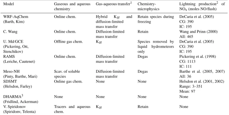
Table 2. Description of chemistry-related processes used by each model.
Model Gaseous and aqueous chemistry
Gas-aqueous transfer1 Chemistry-microphysics
Lightning production2 of NOx(moles NO/flash)
WRF-AqChem (Barth, Kim)
Online chem. Hybrid KH and
diffusion-limited mass transfer
Retain species during freezing
DeCaria et al. (2005) CG: 390
IC: 195 C. Wang Online chem. Diffusion-limited
mass transfer
Retain Wang and Prinn (2000) All: 465
U. Md/GCE (Pickering, Ott, Stenchikov)
Offline gas chem. KH Species removed by
liquid hydrometeors only DeCaria et al. (2005) CG: 390 IC: 195 RAMS (Leriche, Cautenet)
Online chem. Diffusion-limited mass transfer
Degas Pickering et al. (1998) CG: 1113
IC: 111 Meso-NH
(Pinty, Barthe, Mari)
Scav. of soluble species
Diffusion-limited mass transfer
Degas Barthe et al. (2005, 2007) All: 36
SDSMT (Helsdon, Farley)
Online gas chem. None None Helsdon et al. (2001, 2002) Range: 3–351
Mean: 97 DHARMA3
(Fridlind, Ackerman)
None None None None
V. Spiridonov (Spiridonv, Telenta)
Tracers and aqueous chem.
KH Retain None
1K
H indicates that Henry’s law equilibrium is used to partition between gaseous and aqueous phases.
2CG is cloud-to-ground flashes; IC is intracloud flashes; All is both CG and IC flashes.
3Tracers without chemical reactions are included in DHARMA so that comparisons are made with observed species such as CO and O 3,
which are less reactive for the integration time frame.
the top of the domain was not included. The simulation was integrated at a 10 s time step for all the described processes. To keep the convection near the center of the model domain, the grid is moved at 1.5 m s−1eastward and 5.5 m s−1 south-ward.
3.2 C. Wang’s convective cloud model with chemistry
(C. Wang)
The convective cloud model of Wang and Chang (1993a) coupled with chemistry solves the 3-D pseudo-elastic form of the continuity equation. The thermodynamic equations use an ice-liquid potential temperature as a conserved vari-able (Tripoli and Cotton, 1981). A δ four-stream radiation
code Fu and Liou (1993), with predicted O3, water vapor,
and liquid and ice phase hydrometeors, is used to compute the radiation transfer at both short and long waves (Wang and Prinn, 2000). We expect the effects of the radiation scheme on the storm simulation to be small for the 3 h integration. The advection of the chemical species including aerosols is calculated by using a revised Bott scheme (Bott, 1989, 1993) by Wang and Chang (1993a).
The cloud microphysics module predicts both number concentration and mass mixing ratios of cloud particles (e.g.
a 2-moment scheme; Wang and Chang, 1993a). Two liq-uid and two ice phase hydrometeors are represented in the model version for this intercomparison. The precipitating ice hydrometeor has graupel-like characteristics. The aerosol module used for the current simulations has a prognostic CCN (hygroscopic) and IN (insoluble) calculation (Wang and Prinn, 2000). The CCN and IN calculations include transport, nucleation, and precipitation scavenging. The ini-tial surface number concentration of CCN and IN is set to
be 500 cm−3 and 100 L−1, respectively, and is assumed to
be constant from the surface to the top of the model domain. Note that the actual cloud drop activation rate is determined by both the availability of aerosols and temperature as well as the supersaturation at the grid point (Wang, 2005a).
The chemistry sub-model predicts atmospheric concentra-tions of 25 gaseous and 8 aqueous chemical species (in both cloud droplets and raindrops and thus 16 prognostic
vari-ables), undergoing more than 100 reactions of NOx-HOx
-O3-CO-CH4-Sulfur chemistry as well as transport and
mi-crophysical conversions (Wang and Chang, 1993a; Wang et al., 1998a; Wang and Prinn, 2000). Photolysis rates are calculated based on the solar flux determined by the radia-tion module. Dissoluradia-tion of soluble species is parameterized via diffusion-limited mass transfer. When freezing of liquid
hydrometeors occurs, the dissolved gases are assumed to be retained in the frozen hydrometeors. The chemistry mech-anism is solved with the Livermore solver for ordinary dif-ferential equations (LSODE) (Hindmarsh, 1983; Wang et al., 1998a). A module of heterogeneous uptake by ice particles of several key chemical species including O3, H2O2, HNO3,
CH2O, CH3OOH, SO2, and H2SO4based on the first-order
reaction approximation is also included (Wang, 2005b).
The production of NOx from lightning follows the disk
model of Wang and Prinn (2000). The lightning rate is de-rived as a parameterization of actually predicted collision rate between ice crystals and graupel as well as dynamic variables by the model. A prescribed CG/IC ratio (not pre-dicted by the parameterization) of 5% is adopted based on the observation. NO production is set to be 465 moles NO per flash for both IC and CG flash. The freshly-produced NO molecules are distributed vertically based on either two (IC) normal distributions centered respectively at ice crystal and graupel concentrated layers or one (CG) such distribu-tion centered at the latter layer, generally following DeCaria et al. (2000).
The model domain is 145×120 km2 horizontally with a
1 km spatial resolution. The model domain extends from the surface to 20 km with a uniform grid spacing of 400 m. At the top of the model a rigid lid (i.e. w=0) is imposed with a 2.4 km sponge layer to absorb the reflection of gravity waves. The time step for the 3 h integration is 3 s for all the described processes.
3.3 UMd/GCE (K. Pickering, L. Ott and G. Stenchikov)
The UMd/GCE modeling system consists of the 3-D God-dard Cumulus Ensemble (GCE) model (Tao and Simpson, 1993; Tao et al., 2001) and the University of Maryland offline cloud-scale chemical transport model (CSCTM; DeCaria et al., 2005). The output of the GCE model is used to drive the CSCTM.
The GCE model hydrodynamics is based on a complete set of compressible, nonhydrostatic equations in a
Carte-sian coordinate system. A second order finite difference
scheme in the vertical direction and the positive definite non-oscillatory horizontal advection scheme with small im-plicit diffusion (Smolarkiewicz, 1984; Smolarkiewicz and Grabowski, 1990) are employed. Newtonian damping is ap-plied to the potential temperature and components of hor-izontal velocity at the top of the domain at about 25 km. A parameterization of sub-grid turbulent mixing is based on the prognostic equation for turbulent kinetic energy (Deardorf, 1975; Klemp and Wilhelmson, 1978a, b; Soong and Ogura, 1980). Turbulent mixing is handled in the cloud model using a turbulent diffusion approximation.
To parameterize cloud microphysics a Kessler-type scheme (Kessler, 1969; Houze, 1993) for liquid hydromete-ors (cloud water and rain) and the three-category scheme of Lin et al. (1983) for solid hydrometeors (ice, snow, and hail)
are employed. The hydrometeors are assumed to be spheri-cal with exponential size distributions except for cloud water and cloud ice, which are monodisperse. Hail characteristics are used for the simulation.
Output from the 3-D GCE model simulation is used to drive a 3-D Cloud-Scale Chemical Transport Model
(CSCTM, DeCaria et al., 2005). Temperature, density,
wind, hydrometeor (rain, snow, graupel/hail, cloud water, and cloud ice), and diffusion coefficient fields from the GCE model simulation are read into the CSCTM every ten min-utes, and these fields are then interpolated to the model time step of 15 s. The transport of chemical species is calcu-lated using a van Leer advection scheme (Allen et al., 1991). Aerosols are not included in the simulation.
The CSCTM combines transport and lightning produc-tion with a chemical solver (SMVGEAR-II, Jacobson, 1995) and photochemical mechanism to simulate the chemical en-vironment within the storm. The reaction scheme focuses on ozone photochemistry, containing the nonmethane hydro-carbons ethane, ethene, propane, and butane as described in DeCaria et al. (2000, 2005). The chemical scheme involves 35 active chemical species, 76 gas phase chemical reactions, and 18 photolytic reactions. Soluble species are removed from the gas phase by cloud and rain water with a depen-dence on Henry’s Law coefficients. Uptake by ice is not in-cluded. Aqueous and multiphase reactions are not inin-cluded. Photolysis rates are calculated as a function of time and are perturbed by the cloud, using typical summertime estimates from Madronich (1987) and cloud thickness taken from the GCE model output. Initial condition profiles of PAN, ethane, ethene, propane, and butane are from profiles constructed us-ing observations from the 12 July STERAO storm by De-Caria et al. (2005). The single column “spin-up” version of the CSCTM is run for 15 min to allow the chemical concen-trations to come into equilibrium before starting the simula-tion of the storm.
The lightning NO scheme in the CSCTM, described fully in DeCaria et al. (2005), is based on observed flash rate data. CG flash rates are calculated from NLDN observations and IC flash rates are determined by subtracting CG flash rates from total lightning flash rates obtained from interferometer observations. NO from CG flashes is distributed according to a Gaussian distribution peaking in the mid-troposphere while NO from IC flashes is distributed bimodally based on the typical vertical distributions of the VHF sources of IC and CG flashes from MacGorman and Rust (1998). NO from both types of flashes is also distributed vertically pro-portional to pressure. In each model layer, lightning NO is horizontally distributed uniformly to all grid cells with com-puted radar reflectivity greater than 20 dBZ. Production per CG flash (PCG), estimated to be 390 moles NO per flash, is based on the mean peak current of CG flashes observed by the NLDN and a relationship between peak current and en-ergy dissipated (Price et al., 1997). An estimate of NO pro-duction per IC flash (PIC) is obtained by assuming various
PIC/PCG ratios and comparing the results with anvil aircraft measurements. Assuming a PIC/PCG ratio of 0.5 produced
a favorable comparison with observed in-cloud NOxmixing
ratios and as a result, PIC is set to 195 moles NO per flash. The UMd/GCE modeling system was integrated in a
do-main of 360×328×25 km3 in the x, y and z directions,
re-spectively. The horizontal grid spacing was 2 km in both hor-izontal directions, and 0.5 km in the vertical. The GCE mete-orology model was integrated using a 3 s time step to main-tain numerically stability. The chemistry transport model is updated with a 30 s time step (though SMVGEAR-II itself uses a smaller time step based on stiffness).
3.4 RAMS (M. Leriche and S. Cautenet)
Gas and aqueous chemistry have been incorporated into the Regional Atmospheric Modeling System (RAMS) ver-sion 4.3 (Cotton et al., 2003). The basic equations in RAMS for solving the dynamical and thermodynamical variables are non-hydrostatic time-split compressible. The predicted vari-ables are advanced in time via a hybrid leapfrog (on long time step) forward-backward (on short time step), 2nd order flux conservative form (Tripoli and Cotton, 1982). Trans-ported scalars include hydrometeors and chemical species. Aerosols are not simulated for this case.
The cloud microphysics module predicts both number concentration and mass mixing ratios of cloud particles, i.e. a two-moment bulk scheme (Meyers et al., 1997), using gamma distributions to represent the hydrometeor size dis-tributions. For the simulation performed here, the water cat-egories include cloud and rain drops and three ice condensate species: pristine ice, snow, and hail.
The chemistry module includes both gas and aqueous phase chemistry. For gas-phase chemistry, the mechanism includes 29 species with 65 reactions that represent the
reac-tivity of ozone, NOyand VOC including isoprene chemistry
(Arteta et al., 2006; Taghavi et al., 2004). For aqueous-phase chemistry, the mechanism includes 10 species with 18
re-actions that represent the HOxchemistry and the formation
of nitrate, sulfate and formic acid (Audiffren et al., 1998). For the exchange of chemical species between gas phase and liquid hydrometeors, the mass transfer kinetic formulation of Schwartz (1986) is used taking into account the possible deviation from Henry’s law equilibrium. The Quasi-Steady State Approximation (QSSA) is used as the chemical solver. The redistribution of chemical species by microphysical pro-cesses is only considered for liquid hydrometeors. Therefore, when freezing of liquid water occurs, the dissolved species are degassed. The interactions of chemical species with ice phase are not yet implemented in the model.
The lightning-NOxparameterization is based on Pickering
et al. (1998). The parameterization consists of four parts: flash rate, flash type, flash location and NO production rate. The flash rate is computed from the maximum vertical veloc-ity using a power law. The fractions of intracloud (IC) and
cloud to ground (CG) flash are computed by estimating the
depth of the layer from the freezing level (the 0◦C isotherm
in the cloud) to the cloud top. For this storm, the calculation gives ∼4% CG fraction, which is consistent with observa-tions. The CG flashes are placed within the 20 dBZ region
from the surface to the model-calculated −15◦C isotherm
and the IC flashes within the 20 dBZ region of the cloud
above the −15◦C isotherm. The NO production rate is 1113
and 111 moles NO per each CG and IC flash, respectively. For the simulation of the STERAO storm, two
nest-ing grids are used, the large one of 240×240×20 km3
with a horizontal resolution of 3 km and the small one of
120×120×20 km3with a horizontal resolution of 1 km. The
domain has 50 vertical levels with resolution stretching from 50 m at the surface to 1000 m at the top of the domain. A rigid lid (w=0) upper boundary condition is used. The small grid moves into the large one with a constant velocity of
1.5 m s−1 towards the east and 5.5 m s−1southward. A 5 s
time step is used.
3.5 Meso-NH (J.-P. Pinty, C. Barthe and C. Mari)
The Meso-NH model (Lafore et al., 1998) is a complete me-teorological model that contains a flexible chemical scheme, an aerosol scheme, a 1- or 2-moment microphysical scheme and an electrical scheme. The model integrates an anelastic system of equations. The Multidimensional Positive Definite Advection Transport Algorithm (MPDATA; Smolarkiewicz and Grobowski, 1990) is used for the advection scheme, and turbulence is parameterized with a 3-D scheme. Transported scalars include hydrometeors, chemical species and electri-cal charge. Aerosols are not included in this simulation.
The cloud microphysics is described by a mixed-phase scheme (Pinty and Jabouille, 1998) that takes into account 6 water variables (water vapor, cloud droplets, raindrops, pristine ice, snow and graupel). For this study, graupel-like characteristics are used. Only mass mixing ratios of these microphysical species are predicted.
For these simulations, no chemical reactions are consid-ered in the gas and aqueous phases. The partitioning be-tween gas and liquid phases is calculated for the soluble
gases, CH2O, H2O2, and HNO3, following the mass
trans-fer kinetic formalism of Schwartz (1986). The scavenged gases are tracked in the cloud droplets and in the rain drops only, but not in the ice phase. Note that the liquid drops do get transported to the glaciated regions of the modeled storm.
CO and O3are insoluble. NOxis represented by 2 variables:
the first one corresponds to the background NOxand the
sec-ond one includes both background and the NOx produced
from lightning.
Meso-NH also contains an explicit electrification and lightning flash scheme (Barthe et al., 2005). The electric charges are carried by each of the hydrometeor categories and are separated via non-inductive processes (i.e., ice-graupel collisions). Lightning flashes are triggered when the
ambient electric field exceeds a threshold (167ρ(z) kV m−1).
The lightning flashes produce both bi-directional leaders and branch streamers (Barthe et al., 2005). Nitrogen oxides are added along the lightning flash path as a function of the pressure and the channel length as suggested by Wang et al. (1998b) from laboratory experiments (Barthe et al., 2007). The production of NO is 36 moles NO per flash for both CG and IC flashes.
The simulation is configured to that described by
Ska-marock et al. (2000). The computational domain is
160×160×50 grid points with a horizontal resolution of 1 km and a vertical spacing ranging from 75 m at the ground to 700 m in the stratosphere. A gravity wave damping layer is placed between the model top and 15 km height. The time step (2 s) is used for all the described processes.
3.6 SDMST (J. Helsdon and R. Farley)
The 3-D SEM (Storm Electrification Model) has fully cou-pled microphysical, electrical and chemical processes. The model is a modified form of the 3-D nested grid model de-veloped by Terry Clark and associates (Clark, 1977, 1979; Clark and Farley, 1984; Clark and Hall, 1991). The model is nonhydrostatic and uses the anelastic approximation to elim-inate sound waves. For the dynamics, the model employs the flux form of the second-order operators of Arakawa (1966) for the spatial derivatives, and treats time derivatives using a second-order leapfrog scheme. This formulation allows the model to conserve kinetic energy. Advection of scalar quan-tities uses the multidimensional positive-definite advection transport algorithm (MPDATA) developed by Smolarkiewicz (1984) and Smolarkiewicz and Clark (1986). Subgrid-scale turbulence is parameterized according to first-order theory.
The model employs the single moment (mixing ratio) mi-crophysical parameterization scheme of Lin et al. (1983) which allows five hydrometeor classes; cloud water, rain, cloud ice, snow, and graupel/hail. For the simulation reported here, the model uses parameters characteristic of hail to rep-resent the graupel/hail field.
Gas phase chemical processes are included in the model as described in Zhang et al. (2003). This formulation has 18 reactions involving nine tracked chemical species including
NO, NO2, O3, CH4, CO, OH and HO2, with HNO3as a sink.
The chemistry solver is a modified QSSA solver. The re-sulting equation set is solved using a 2nd order Runge-Kutta scheme with the time step controlled by the stiffness of the chemistry equations.
The treatment of electrical processes follows Helsdon and Farley (1987) and Helsdon et al. (2001). Each hydrome-teor class has an associated charge density in addition to the positive and negative small ion concentrations that com-bine to form the total charge density, which is related to the electrical potential through Poisson’s equation. The simu-lation includes an explicit prediction of intracloud lightning discharges as described in Helsdon et al. (1992) and
Hels-don et al. (2002). A lightning channel is initiated when and
where a threshold electric field is attained (225 kV m−1 in
this case) and propagates bi-directionally away from the ini-tiation point following the electric field vector. The channel terminates when the electric field at the ends of the
propagat-ing channel drops below a preset value (75 kV m−1). Once
the channel is formed, its linear charge density is calculated from theory and converted into an equivalent small ion den-sity. The charged channel modifies the electric field and consequently modifies the electric energy in the domain in a physically consistent manner. By calculating the electri-cal energy just before and immediately after the discharge, the energy dissipation can be determined. NO production
(9×10¹⁶ NO molecules J−1 at sea level) is proportional to
this electrical energy change and pressure, and is limited to the immediate vicinity of the lightning channel. For this sim-ulation, the NO production ranges from 5 to 351 moles NO per flash with a mean of 97.
The simulation is configured to a 120×120×20 km3
do-main using 1 km horizontal grid spacing and 250 m vertical resolution. At the top of the model, a 4-km deep Rayleigh friction upper level absorber for the velocity components and potential temperature is used. The model integrations pro-ceed using a 2 s time step. A Galilean transformation is ap-plied to keep the main convection within the interior regions of the domain. For the 10 July STERAO case the grid trans-lates to the east at 4 m s−1and to the south at 5 m s−1.
3.7 DHARMA (A. Fridlind and A. Ackerman)
The DHARMA (Distributed Hydrodynamic
Aerosol-Radiation-Microphysics Application) model treats atmo-spheric and cloud dynamics with a large-eddy simulation code (Stevens and Bretherton, 1996) that solves an anelastic approximation of the Navier-Stokes equations appropriate for deep convection (Lipps and Hemler, 1986).
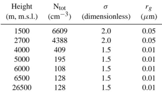
Embedded within the dynamics code, DHARMA treats aerosol and cloud microphysics with the CARMA (Commu-nity Aerosol-Radiation Model for Atmospheres) code (Ack-erman et al., 1995; Jensen et al., 1998). Aerosols, water drops, ice crystals, and solute within the drops and crystals are tracked in a range of sizes (16 size categories each). The aerosols are assumed to be ammonium bisulfate distributed log-normally (dry size). The initial concentration and size distribution parameters of the aerosol are listed in Table 3 and are based on the condensation nuclei measurements on the aircraft. The density of ice is a function of size, roughly representative of conical graupel. Microphysical processes include aerosol activation into drops, condensational growth and evaporation of drops, gravitational collection, sponta-neous and collision-induced drop breakup, homogesponta-neous and heterogeneous freezing of aerosols and drops, deposi-tional growth and sublimation of ice, sedimentation of liquid and ice, melting, and Hallett-Mossop rime splintering. The
microphysics treatment is identical to that used by Fridlind et al. (2004), where further detail is provided.
The DHARMA model transports aerosols, hydrometeors,
and trace gases. Chemistry and production of NOx from
lightning are not included in the model.
Results shown here are for uniform 1 km horizontal
resolu-tion and 250 m vertical resoluresolu-tion over a 120×120×20 km3
domain, which is nudged to the initial profile along each face. The boundary condition at the top of the model is a rigid lid (w=0). Dynamics and gravitational collection are advanced with a 5 s time step; all other microphysical processes are ad-vanced with a time step of 0.2 to 5 s that is chosen based on the processes that are active in each grid cell as the simula-tion progresses.
3.8 V. Spiridonov’s convective cloud model with chemistry
(V. Spiridonov and B. Telenta)
The model (Spiridonov and Curic, 2003, 2005) is a three-dimensional, non-hydrostatic, time-dependant, compressible system using the dynamic and thermodynamics schemes from Klemp and Wilhelmson (1978a) and the bulk cloud mi-crophysics scheme from Lin et al. (1983) that takes into ac-count 6 water variables (water vapor, cloud droplets, ice crys-tals, rain, snow, and graupel). The graupel hydrometeor class is represented as hail with a density of 0.9 g cm−3. While the mass of aerosol sulfate is predicted, the aerosols do not affect the cloud drop activation. The chemistry module includes 4 species (SO2, SO2−4 , NH+4, H2O2) and 3 aqueous-phase
re-actions describing in-cloud sulfate chemistry (Taylor, 1989). The absorption of chemical species from the gas phase into cloud water and rainwater is determined by either Henry’s law equilibrium (Taylor, 1989), or by diffusion-limited mass transfer between gas and liquid phases to include possible non-equilibrium states, (Barth et al., 2001). All equilibrium constants and oxidation reactions are temperature dependent according to the van’t-Hoff relation (Seinfeld, 1986). Cloud water and rainwater pH is calculated using the charge balance equation from Taylor (1989). The model includes a freezing transport mechanism of chemical species based on Rutledge et al. (1986). Thus, when water from one hydrometeor class is transferred to another, the dissolved scalar is transferred to the destination hydrometeor in proportion to the water mass that was transferred. Production of NO from lightning is not parameterized in the Spiridonov model.
For the intercomparison simulation, the model is
config-ured to a domain of 140×140×15 km3with 1 km horizontal
resolution and 500 m vertical resolution. A rigid lid (w=0) is used for the top boundary condition. A 10 s time step is used for all the described processes.
Table 3. Aerosol parameters used for initialization in the DHARMA model. Height Ntot σ rg (m, m.s.l.) (cm−3) (dimensionless) (µm) 1500 6609 2.0 0.05 2700 4388 2.0 0.05 4000 409 1.5 0.01 5000 195 1.5 0.01 6000 108 1.5 0.01 6500 128 1.5 0.01 26500 128 1.5 0.01
Ntotis the total concentration, σ is the geometric standard deviation,
and rgis the geometric mean radius of the aerosol size distribution.
4 Results
Four types of model results are presented. First, the storm intensity and structure are analyzed by intercomparison of peak vertical velocity and radar reflectivity with
observa-tions. Second, the redistribution of CO, O3 and NOx are
presented, and anvil mixing ratios are compared with ana-lyzed UND Citation aircraft measurements. Then the flux of
air, CO and NOxthrough a plane across the anvil is compared
to that determined from the observations. Lastly the mixing
ratios of CH2O, H2O2, and HNO3in the anvil are compared
among models.
4.1 Storm intensity and structure
The maximum vertical velocity in the model domain was recorded at 10-min intervals (Fig. 2). Each model shows a rapid increase in peak updraft velocity at the beginning
of the simulation. Most simulations maintain peak
up-drafts above 24 m s−1 during the remainder of the
simula-tion, while radar observations show peak updrafts to be
be-tween 24 and 38 m s−1. Transitions to updraft velocities
of 35 m s−1 or more are seen by C. Wang’s model,
WRF-Aqchem, DHARMA, and Meso-NH. The height of the peak updraft ranges from 7 km to 14 km m.s.l., which is similar but somewhat higher than observations.
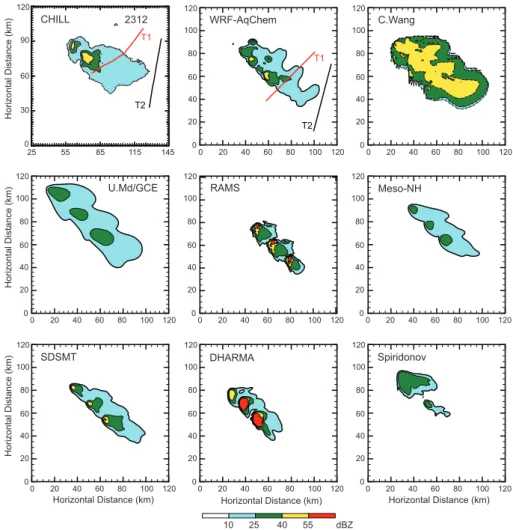
The storm structure can be evaluated by comparing the modeled radar reflectivity to the observed radar reflectivity. Both horizontal and vertical cross-sections of radar reflectiv-ity are examined. At 23:12 UTC 10 July, the CSU CHILL radar reflectivity at z=10.5 km m.s.l. indicates two convec-tive cores oriented in a northwest-southeast line with an anvil spreading to the east-southeast (Fig. 3). However, during the multicell stage of the storm 2 to 4 convective cells were ob-served. After 1 h of simulation, the results from the mod-els have 2–3 convective cores oriented northwest-southeast which is in line with the observations. The magnitude of the reflectivity differs among models due to 1) whether graupel
Fig. 2. (a) Peak updraft speed and (b) height of peak updraft from each of the simulations. Gray shaded regions represent observed values derived from the CHILL radar (W. Deierling, personal communication).
characteristics (C. Wang, Meso-NH, DHARMA models) or hail characteristics are modeled, 2) model resolution, and 3) single-moment versus multi-moment (C. Wang, DHARMA, RAMS models) microphysics parameterizations. The width of the anvil varies among models. The observed reflectivity has an anvil width of 32–40 km at 23:12 UTC, while model results range from 12.5 km to 45 km. Seifert and Weisman (2005) noted that double-moment microphysics parameteri-zations tend to produce broader anvils than single-moment microphysics parameterizations. The results from our study do not distinctly show this correlation. While C. Wang’s model with double-moment microphysics has a widespread anvil, DHARMA and RAMS have anvils similar in width to the models with single-moment microphysics. Other factors contributing to the anvil width are the graupel or hail charac-teristics used (which influences the particle’s fall speed), the dynamics formulation, the vertical or horizontal resolution, and the number of bubbles used to initiate the convection. For example, a sensitivity simulation with a 2-bubble initi-ation performed by WRF-Aqchem found that the anvil was less extensive in both the length and width than the 3-bubble initiation used in the intercomparison exercise.
The vertical cross section of observed reflectivity along the storm axis (Fig. 4) shows that the northwest core (left side of figure) is decaying while the southeast core is reaching its mature stage. During the multicell stage of the storm, radar reflectivity plots show 2 to 4 convective cores being active at any given time. All of the models show 3 convective cores, with all cores of approximately the same reflectivity magni-tude except for the Meso-NH model. The Meso-NH model has weaker reflectivity most likely because of the graupel (rather than hail) characteristics used in their microphysics parameterization. While the reflectivity in the observed anvil
is weak (5–20 dBZ) and somewhat extensive (>35 km from the southeast core to the anvil edge), the simulated anvils are stronger (5–35 dBZ) and less extensive (15–25 km from the southeast core to the anvil edge). The maximum height of the modeled reflectivity varies among models. The reflectivity simulated by Spiridonov only reaches 11.5 km, m.s.l., while the reflectivity simulated by the C. Wang and RAMS models reach 16.5 km, m.s.l. Observations show the reflectivity top to be 14.5 to 16.5 km, m.s.l.
In summary, the discrepancies among models for radar re-flectivity, which are mainly due to the differences between the treatments of cloud microphysics, highlight the response of different cloud models to the same initiation protocol and the challenge of modeling the realistic structure of clouds even using cloud resolving models. Nevertheless, the mod-eled cloud structures are all reasonably simulated. Thus, it is possible to use these models to simulate trace gas transport as part of the intercomparison.
4.2 Distributions of CO, O3, and NOx
Mixing ratios of gas-phase CO, O3, and NOxare compared to
observations using two approaches. First, model results are evaluated with aircraft measurements which were obtained from the University of North Dakota (UND) Citation aircraft as it flew across the anvil. Second, cross-sections of the gas-phase mixing ratios are compared to a derived cross-section obtained from several transects of the anvil by the aircraft.
The UND Citation aircraft sampled the outflow region of the storm by performing across-anvil transects at different levels in the anvil (transects indicated in Fig. 3). Two tran-sects are used to compare model results with observations. The first transect is 10 km downwind of the southeastern-most convective cell at 23:10 UTC (which corresponds to
25 55 85 115 145 0 30 60 90 120 2312
CHILL WRF-AqChem C.Wang
U.Md/GCE RAMS Meso-NH
SDSMT DHARMA Spiridonov 0 20 60 80 120 40 100 0 20 60 80 120 40 100 0 20 40 60 80 100 120 0 20 40 60 80 100 120 0 20 60 80 120 40 100 0 20 60 80 120 40 100 0 20 40 60 80 100 120 0 20 40 60 80 100 120 0 20 60 80 120 40 100 0 20 60 80 120 40 100 0 20 40 60 80 100 120 0 20 40 60 80 100 120 0 20 60 80 120 40 100 0 20 40 60 80 100 120 0 20 60 80 120 40 100 0 20 40 60 80 100 120 10 25 40 55 dBZ
Horizontal Distance (km) Horizontal Distance (km) Horizontal Distance (km) Horizontal Distance (km) Horizontal Distance (km) Horizontal Distance (km) T1 T2 T1 T2
Fig. 3. Radar reflectivity (dBZ) at z=10.5 km m.s.l. Observations (upper left panel) from CSU CHILL radar at 23:12 UTC. Model results at
t =1 h from WRF-AqChem, C. Wang, UMd/GCE, RAMS, Meso-NH, SDSMT, DHARMA, and Spiridonov models. T1 and T2 lines in the
CHILL panel represent the actual flight track for the two transects shown in subsequent figures. T1 and T2 lines in the WRF-AqChem panel represent the location of the modeled transects shown in the same subsequent figures.
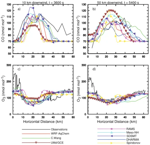
t =1 h in the simulations) at 11.6 km m.s.l. The second tran-sect is ∼50 km downwind of the southeastern-most convec-tive cell at 2335 UTC (corresponding to t=1 h 30 min in the simulations) at 11.2 km m.s.l. One would expect that the model results discussed below are dependent on the chosen location of transect. The horizontal variability of a species in the anvil can be fairly large (Barth et al., 2007) as the storm dynamics and entrainment can vary with time. The choice of the location for the across-anvil transect in each model is that which is most appropriate at the ∼10 km and ∼50 km downwind location to compare to the available observations. Mixing ratios of gas-phase CO in the anvil are observed to be enhanced compared to the background upper tropo-sphere (Fig. 5) because convective transport moves high mix-ing ratios from the boundary layer to the upper troposphere.
Conversely, gas-phase O3 mixing ratios are lower in the
anvil than in the upper troposphere because relatively-low
O3 mixing ratios are transported from the boundary layer.
The model simulations predict these enhancements and
de-pletions of CO and O3 mixing ratios, which agree with the
observations (Fig. 5), especially in the core of the anvil. All
models underpredict the O3 mixing ratio on the southwest
edge of the anvil, a feature that may be attributed to mix-ing of stratospheric air. The results from the models can be sensitive to the time and location of the transect. For exam-ple, the horizontal distribution of CO at z=11.5 km shown in Barth et al. (2007) illustrates heterogeneity as CO is en-trained/detrained during transport from the boundary layer to the anvil. Keeping these sensitivities in mind, the model results are within 10–15% of the observations in the anvil.
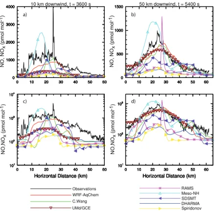
Observed gas-phase NO mixing ratios (Fig. 6) are strongly enhanced within the anvil compared to the background up-per troposphere primarily due to lightning production of NO.
Modeled gas-phase NOxmixing ratios show the importance
of the lightning source. The DHARMA and Spiridonov
Observations 16.5 11.5 6.5 1.5 16.5 11.5 6.5 1.5 16.5 11.5 6.5 1.5 0 20 40 60 80 100 0 20 40 60 80 100 0 20 40 60 80 100 WRF-AqChem C.Wang
U.Md/GCE RAMS Meso-NH
SDSMT DHARMA Spiridonov
Horizontal Distance (km) Horizontal Distance (km)
Horizontal Distance (km) Height (km, m.s.l.) Height (km, m.s.l.) Height (km, m.s.l.) 5 20 35 50 dBZ 2312 UTC
Fig. 4. Radar reflectivity (dBZ) along the NW-SE vertical cross-section. Observations (upper left panel) from CSU CHILL radar at 23:12 UTC. Model results at t =1 h from WRF-AqChem, C. Wang, UMd./GCE, RAMS, Meso-NH, SDSMT, DHARMA and Spiridonov models.
and therefore substantially underpredict the NOxmixing
ra-tios. The increase in NOx seen within the anvil region
for the DHARMA and Spiridonov models is a result of
transport of boundary layer NOx to the upper troposphere.
The other models, which include lightning-produced NOx,
generally show NOxmixing ratios elevated compared to the
DHARMA and Spiridonov models within the anvil. For
the first transect, WRF-AqChem, C. Wang, Meso-NH, and
SDSMT NOx mixing ratios are similar to the observations,
but for shorter across-anvil distances. Only the Meso-NH model has a similar area under the curve as the observations,
indicating the total amount of NOxplaced into the 11.6 km
m.s.l. height is realistic (note that mass fluxes of NOx
inte-grated over the across-anvil area and over time are discussed in the next section). For the second transect, all of the models
that include NOx production by lightning agree reasonably
well with observations. The results from the RAMS model are generally lower than the other models with a
lightning-NOxproduction scheme. The details of the RAMS
lightning-NOx parameterization (Pickering et al., 1998) indicate that
small amounts of NO (111 moles NO/IC flash) are produced
and placed in a large volume (above −15◦C isotherm for
cloud regions >20 dBZ (Fig. 4)) leading to a reduced NOx
mixing ratio. The UMd/GCE model produces more NO per IC flash (195 moles/flash) but concentrations are reduced be-cause of the large volume of cloud >20 dBZ (Fig. 4). In addition, variations from the models can be a result of the location and time of the model transect as is discussed above with the CO transect. This is the first time simulated
light-ning NOxproduction from a specific model transect has been
directly compared with observations from the corresponding
specific aircraft transect of a storm anvil. To obtain NOx
mixing ratios similar in magnitude to observations is encour-aging. These results highlight that several key parameters (lightning flash rate which depends on the storm kinematic and microphysical characteristics, lightning type, NO source location, NO production per lightning flash) need to be
incor-porated in lightning-NOx parameterizations, and that these
same parameters play an important role in contributing to
un-certainties in NOxmixing ratios in convective outflow.
Skamarock et al. (2003) analyzed the UND Citation air-craft data taken across the anvil of the storm. The Citation aircraft mapped out the anvil structure during ∼1 h 30 min time period by traversing the anvil in horizontal passes, ap-proximately perpendicular to the long axis of the anvil, at elevations starting at approximately 11.8 km m.s.l. (close to the anvil top) and ending at approximately 6.8 km m.s.l. Skamarock et al. (2003) projected the cloud particle
concen-tration, CO, O3, and NO observations onto a vertical plane
using an objective analysis procedure. Uncertainties related to this methodology are associated with the temporal evo-lution of the storm while the measurements were taken and with the background state of each constituent measured. Ska-marock et al. (2003) conclude that these uncertainties are fairly small resulting in a reasonable flux analysis. Model predictions of these variables taken along a similar plane (similar to the T2 cross-section shown for WRF-AqChem in Fig. 3) can then be compared to the analyzed observations.
Vertical cross-sections across the anvil of ice particle con-centration are shown in Fig. 7. The analyzed observations are
for ice >25 µm diameter (Dice) based on the measurements
d) a) b) c) CO (nmol mol -1) O3 (nmol mol -1)
Horizontal Distance (km) Horizontal Distance (km)
CO (nmol mol
-1)
O3
(nmol mol
-1)
Fig. 5. CO and O3 measurements (black lines) from the UND-Citation aircraft for across-anvil transects at 10 km downwind of the south-easternmost convective cell and 11.6 km m.s.l. (left panels) and at 50 km downwind of the south-easternmost convective cell and 11.2 km m.s.l. (right panels). Results from model calculations are plotted along these transects.
2000). The results from the models tend to match or over-predict the observations. The results from the C. Wang and
RAMS models are only for Dice>25 µm giving good
agree-ment with observations. While the DHARMA results are
also only for ice with Dice>25 µm, the results overpredict
the ice particle number, suggesting other factors contribute to increased predicted ice particle number. Using graupel char-acteristics instead of hail can also increase ice concentrations in the anvil region because graupel has a smaller fall speed and therefore is carried further into the anvil. The models that predicted only the mass of the cloud particles (WRF-AqChem, UMd/GCE, Meso-NH, SDSMT, Spiridonov) as-sumed a diameter for the ice hydrometeor category (for
ex-ample, WRF-AqChem set Dice=45 µm) for the purposes of
estimating the number concentration. The calculation of
number concentration is very dependent on the assumed ice diameter since the anvil is primarily composed of small ice particles.
Gas-phase CO analyzed from the observations (Fig. 8)
reach 110 nmol mol−1or so in the anvil. Simulated CO
mix-ing ratios also reach those values in the anvil. There is a slight
underprediction of CO seen in the WRF-AqChem model. In general, the models reasonably simulate CO mixing ratios in the anvil.
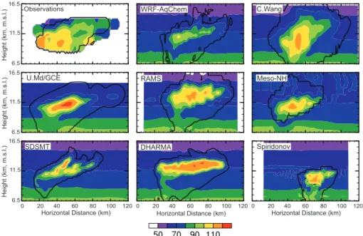
Vertical cross-sections of observed O3 (Fig. 9) show
O3 being depleted in the anvil to values of about
80–100 nmol mol−1, but also show a small region of
downward-intruding, high (>300 nmol mol−1) O3at the top
of the anvil on the SSW edge (upper left part of figure).
Simulated O3mixing ratios range from 60–100 nmol mol−1
within the anvil, similar to observations. Only the C. Wang
and RAMS models show some downward intrusion of O3on
the SSW upper edge of the anvil (note the change in verti-cal gradient of O3at z=13.5 km, m.s.l. on the left side of the
anvil). Because of the lack of additional observations (par-ticularly above the anvil), it is difficult to conclude what
pro-cesses contribute to the observed high levels of O3at the top
of the SSW edge of the anvil.
The analyzed gas-phase NO mixing ratios from
observa-tions have peaks of NO of over 500 pmol mol−1 (Fig. 10)
within a broad region of NO>200 pmol mol−1. Note that
d) a) b) c) NO, NO x (pmol mol -1) NO,NO x (pmol mol -1) NO, NO x (pmol mol -1) NO,NO x (pmol mol -1)
Fig. 6. NO measurements (black lines) from the UND-Citation aircraft for across-anvil transects at 10 km downwind of the south-easternmost convective cell and 11.6 km m.s.l. (left panels) and at 50 km downwind of the south-easternmost convective cell and 11.2 km m.s.l. (right panels). Results from model calculations of NOxare plotted along these transects. NOxis plotted on a linear scale in the upper panels, and
on a logarithmic scale in the lower panels.
Observations 16.5 11.5 6.5 16.5 11.5 6.5 16.5 11.5 6.5 0 20 40 60 80 100 120 0 20 40 60 80 100 120 0 20 40 60 80 100 120 WRF-AqChem C.Wang
U.Md/GCE RAMS Meso-NH
SDSMT DHARMA Spiridonov
Horizontal Distance (km) Horizontal Distance (km)
Horizontal Distance (km)
Height (km, m.s.l.)
Height (km, m.s.l.)
Height (km, m.s.l.)
Fig. 7. Cloud particle concentration (per liter) across the anvil at t=23:16 to t=00:36 UTC for the observations and t =6000 s for the model results. The location of the cross-section is similar to transect 2 (T2) shown in Fig. 3. The solid black line is cloud particle concentration equal to 0.1 per liter. Objective analysis of the aircraft measurements (upper left panel) are from Skamarock et al. (2003). Model results are for the WRF-AqChem, C. Wang, UMd/GCE, RAMS, Meso-NH, SDSMT, DHARMA, and Spiridonov models.
Observations 16.5 11.5 6.5 16.5 11.5 6.5 16.5 11.5 6.5 0 20 40 60 80 100 120 0 20 40 60 80 100 120 0 20 40 60 80 100 120 WRF-AqChem C.Wang
U.Md/GCE RAMS Meso-NH
SDSMT DHARMA Spiridonov
Horizontal Distance (km) Horizontal Distance (km)
Horizontal Distance (km)
Height (km, m.s.l.)
Height (km, m.s.l.)
Height (km, m.s.l.)
Fig. 8. Same as Fig. 7 except for CO (nmol mol−1). The solid black line is cloud particle concentration equal to 0.1 per liter.
Observations 16.5 11.5 6.5 16.5 11.5 6.5 16.5 11.5 6.5 0 20 40 60 80 100 120 0 20 40 60 80 100 120 0 20 40 60 80 100 120 WRF-AqChem C.Wang
U.Md/GCE RAMS Meso-NH
SDSMT DHARMA Spiridonov
Horizontal Distance (km) Horizontal Distance (km)
Horizontal Distance (km)
Height (km, m.s.l.)
Height (km, m.s.l.)
Height (km, m.s.l.)
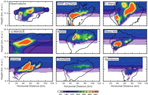
Fig. 9. Same as Fig. 7 except for O3(nmol mol−1). The solid black line is cloud particle concentration equal to 0.1 per liter.
NOx. By assuming photochemical equilibrium between NO
and NO2, NOxmixing ratios are 1.1 to 1.6 times greater than
NO mixing ratios (Skamarock et al., 2003). Thus, modeled
gas-phase NOx should be ∼30% greater than the observed
NO in the middle of the anvil. Results from models that did
not include production of NOxfrom lightning (DHARMA,
Spiridonov) do not predict the NOx>500 pmol mol−1peaks,
but instead show NOx∼200 pmol mol−1 in the anvil; much
less than that observed. The models with production of
NOx from lightning (WRF-AqChem, C. Wang, UMd/GCE,
RAMS, Meso-NH and SDSMT) do predict peaks of NOxon
the same order of magnitude as the observations. These
mod-els also have a broad region of NOxmixing ratios between
150 and 250 pmol mol−1, similar to those seen in the
obser-vations. To obtain the observed peak values of the NOx,
pro-duction from lightning must be modeled.
4.3 Mass fluxes in the anvil outflow
Utilizing the modeled mixing ratio (C) in the anvil cross-sections (shown in Figs. 8–10) and the horizontal velocity
Observations 16.5 11.5 6.5 16.5 11.5 6.5 16.5 11.5 6.5 0 20 40 60 80 100 120 0 20 40 60 80 100 120 0 20 40 60 80 100 120 WRF-AqChem C.Wang
U.Md/GCE RAMS Meso-NH
SDSMT DHARMA Spiridonov
Horizontal Distance (km) Horizontal Distance (km)
Horizontal Distance (km)
Height (km, m.s.l.)
Height (km, m.s.l.)
Height (km, m.s.l.)
Fig. 10. Same as Fig. 7 except for NO, NOx. Observations show NO mixing ratios (pmol mol−1) and models show NOx. The solid black
line is cloud particle concentration equal to 0.1 per liter.
mass fluxes can be made. Corresponding mass fluxes of air,
CO, and NOx are derived from the aircraft measurements
(Skamarock et al., 2003) for comparison to the model results. The calculation of the modeled mass flux density is
flux = P anvil cells ρ U⊥C 1ℓ 1z P anvil cells 1ℓ 1z
where 1ℓ and 1z are the horizontal and vertical grid cell spacing within the anvil. The flux density is determined only in the region where cloud particles exist in the anvil.
Table 4 lists the anvil area as well as the fluxes of air mass,
CO, and NOxaveraged over a 1 h time period, which is
com-parable to the time period of the aircraft measurements. Each model’s average mass flux can be compared to the mass flux derived from observations, which was determined by Ska-marock et al. (2003) from the analyzed cross section.
While the analyzed anvil area taken from the observations
is 315 km2, the modeled anvil area ranges from 109 km2
to 590 km2, which are within −65 and 90% of the
ana-lyzed observed area. The air mass flux determined from the observations is 5.9 kg m−2s−1, while those predicted by
the models range from 6.6 to 9.1 kg m−2s−1. Note that
there is also some uncertainty in the observed anvil area and flux densities (Skamarock et al., 2003) associated with uncertainties in the in situ measurements and in temporal changes in these measured species and in the anvil cross-section area as the measurements were taken. All of the models overpredict the air mass flux, suggesting that the modeled wind speeds in the anvil are too strong. The CO flux density calculation from the observational analysis is
1.9×10⁻⁵moles m−2s−1, while the modeled CO flux
den-sities range from 1.93 to 2.8×10⁻⁵moles m−2s−1. We find that 4 models are within 5% of the analyzed CO flux
den-sity and a total of 7 models are within 33%. However,
because the air mass flux is over-predicted by all mod-els, a correction to the air mass flux density would re-sult in CO flux densities for all models being smaller than
the analysis of the measurements. The NOx flux
den-sity derived from the observations includes NOx produced
from lightning and has a value of 5.8×10⁻⁸moles m−2s−1.
The NOx flux densities determined from models
with-out lightning-NOxproduction (DHARMA, Spiridonov) are
4.3×10⁻⁸ and 2.7×10⁻⁸moles m−2s−1, while the models
that do include lightning-NOx production are between 3.9
and 13.0×10⁻⁸moles m−2s−1. We find that the variability
among the modeled NOxflux densities is clearly higher than
that for the air mass or CO flux densities.
One of the unique features of this intercomparison exercise is that of the 6 models that simulated lightning production
of NOx there are 5 different schemes used. Two schemes
(Meso-NH and SDSMT) explicitly predict the charge coin-cident with the hydrometeors, locate the NO source along the lightning channel using a fairly small NO production value (36 and 97 moles NO/flash for Meso-NH and SDSMT, respectively). The WRF-AqChem and UMd/GCE models
use the same lightning-NOx parameterization in which
ob-served lightning flash rates are used as input and catego-rized as CG or IC flashes. The NO produced from lightning is uniformly placed in the >20 dBZ region with Gaussian (CG) or bimodal (IC) vertical distributions. Fairly high pro-duction of NO (395 moles NO/CG flash; 195 moles NO/IC