HAL Id: tel-00010384
https://tel.archives-ouvertes.fr/tel-00010384
Submitted on 4 Oct 2005
HAL is a multi-disciplinary open access archive for the deposit and dissemination of sci-entific research documents, whether they are pub-lished or not. The documents may come from teaching and research institutions in France or abroad, or from public or private research centers.
L’archive ouverte pluridisciplinaire HAL, est destinée au dépôt et à la diffusion de documents scientifiques de niveau recherche, publiés ou non, émanant des établissements d’enseignement et de recherche français ou étrangers, des laboratoires publics ou privés.
Application of Mach-Zehnder interferometer for
co-phasing extremely large telescopes
Luzma Montoya-Martinez
To cite this version:
Luzma Montoya-Martinez. Application of Mach-Zehnder interferometer for co-phasing extremely large telescopes. Astrophysics [astro-ph]. Université de Provence - Aix-Marseille I, 2004. English. �tel-00010384�
ÉCOLE DOCTORALE « Physique et sciences de la matière »
Application de l’interféromètre de Mach-Zehnder
au co-phasage des grands télescopes segmentés
THÈSE
pour obtenir le grade de Docteur de l’Université de Provence Discipline: rayonnement et plasmas-optique
Présentée et soutenue publiquement le 20 septembre 2004 par
LUZ MARÍA MONTOYA-MARTÍNEZ
Directeurs de thèse : GÉRARD LEMAITRE et KJETIL DOHLEN
JURY
M. Claude Aime président
M. Salvador Cuevas Cardona rapporteur
M. Nicholas Devaney rapporteur
M. Gérard Rousset examinateur
M. Kjetil Dohlen co-directeur de thèse
A mis padres,
a Cris y Marian,
a Jorge
.I would like first to thank the RTN Program, “Adaptive Optics for ELts”, the financial support of this work and for the opportunity of meeting other members of the Network.
Je veux remercier mon directeur de thèse, Gérard Lemaitre, pour son accueil et son soutien tout au long de la thèse.
A Kjetil je lui dois plus qu'un remerciement. Sans lui je ne serais jamais arrivée jusqu'au bout. Lui, il m'a appris à réfléchir et à ressortir l'esprit critique, très important pour la recherche. Même s'il avait toujours plein de choses à faire, il trouvait le temps pour se consacrer à moi. Merci aussi pour la patiente qu'il a montrée même dans les moments ou je sortais les plus grandes bêtises. Je ne peux dire que ¡BRAVO!.
A tout le personnel du Labo. A Marc pour le soutien moral qui a été très important pour moi. A Fred pour sa disponibilité inconditionnelle. A Patrick parce que sans lui le chapitre 4 n'existerai pas. Il m'a montré comme il faut travailler au banc optique sans désespérer. A Silvio et Valerie pour l’aide informatique. A Arnaud pour être mon Born & Wolf et pour son aide précieuse avec la présentation oral de cette thèse. A Léo María parce qu'il m'a beaucoup aidée avec le super résumé en français. Au début il a été mon IDL guideline mais finalement il est devenu un très bon ami. A Christine pour son soutien quotidien. A Olivia et sa famille pour les soirées à La Ciotat et sa joie.
I would like to thanks all the RTN members. Specially Marcel for his support with CAOS, Rodolph for this useful experience with turbulence, Natalia for her warm help in Fourier Optics, Markus for the great support in IDL, Nicholas and GTC staff for the nice welcome at La Laguna and all I learnt with them, Dolo because she is an excellent reference for my work, Achim because it is a pleasure to work with him and he is always available to resolve my questions.
Pero si en una tesis el trabajo intelectual es importante, desde luego el moral no es menos. En este sentido doy las gracias a todos los que me han apoyado y han soportado mis quejas desde lejos.
Así que gracias a Cami, Inés, Lauri, La Rubia, Nuria, Maribel y Gaspi porque nunca dudaron que yo lo conseguiría y me han mimado y animado siempre que estaba triste. Porque me ha hecho reir y ha sido mi fiel compañera de “perjudicamiento”, le doy las gracias a Elena. Menos mal que Lorenzo y Maria del Mar estaban en Barcelona para hacer el retorno de vacaciones a Marsella mucho mas llevadero.
Un agradecimiento muy cariñoso para Ángeles, Ruth, Carlos, Jesús, Luis y todos los demás que hicieron mi estancia en Canarias tan agradable.
No me olvido de las chelas y las “soires en l’Intermédiaire” con los pinches mejicanos, Jorge y Leo y el canijo de Marc. A pesar de que se fueron muy lejos, Iqui y Marcela se quedaron muy cerca y forman parte de los momentos mas intensos vividos en Marsella. Y que decir de Juanjo “el gato”, el primer español que conocí en Marsella y que me cuido como un padre hasta que llego Jorge.
A mis compis del Calar Alto, Jesus, Santos, Manolo, Felipe, Ulli y Alberto les doy las gracias porque a pesar de estos cuatro años fuera siguen queriendo que vuelva... bueno unos mas que otros.
A Begoña, porque aunque nunca vino a verme siempre estuvo conmigo.
A los “cousins”, Jeremy, Ricki, Ludo, Leo et Julie porque mereció la pena venir a Marsella solo por conocerles.
A los Strehle por las comidas tan ricas que nos hicieron con la famosa “canicule” y porque junto con Christian y Barbara lo pasamos muy bien de fiesta en fiesta. Y por supuesto
todo este lío no habría empezado sin la generosa ayuda de mi familia alemana, Los Gutjahr, que un día cambiaron mi destino.
A mis queridos vecinos, Sabine, Stephane, Galawesh y Tanguy que hicieron que mi estancia en Marsella fuera mucho mas agradable de lo que yo siempre les dije.
Para terminar quiero acordarme de Yann, porque fue mi compañero de despacho preferido, porque fue mi primer amigo francés, porque me enseño el francés que hablo y porque sin el todo habría sido todavía mas difícil.
A mis padres quiero dedicarles este trabajo por aguantar tantos llantos, lamentos y quejas con tanto cariño. A mi abuela por su velas milagrosas. A mi hermana Cris le agradezco todo el trabajo de traducción de esta tesis y sus palabras tiernas de animo y a mi hermana Marian su manera tan peculiar de animarme, “pues neno acaba ya”.
Y a ti Garbancito, mas gracias que a nadie, porque lo has hecho muy bien, porque hiciste la integral circulo, porque te leíste mil veces la tesis, porque escuchaste siete veces la presentación, porque me aguantaste mas que nadie y porque sin ti desde luego nunca la hubiera terminado.
Résume
La segmentation des miroirs semble être l’unique solution envisageable pour les très grands télescopes. Pour obtenir la qualité d’image nécessaire aux programmes scientifiques astronomiques, les erreurs d’alignement des segments doivent être réduites à la dizaine de nanomètres.
Cette thèse présente une nouvelle technique pour le co-phasage des miroirs segmentés basée sur un interféromètre de Mach-Zehnder comportant un filtre spatial dans un des bras. Les perturbations atmosphériques sont éliminées si la taille de filtre est de l’ordre de la tache de seeing. L’étude a été divisée en trois niveaux: étude analytique, simulation numérique et approche expérimentale. La performance de cette technique a été étudiée pour des cas réalistes en considérant les effets de bords, le bruit de photon et les caractéristiques du détecteur.
Une comparaison de trois nouvelles techniques de co-phasage est aussi présentée. Cette technique semble être un des candidats les plus prometteurs pour des grands télescopes segmentes.
Abstract
Segmentation seems to be the unique solution for Extremely Large Telescopes (ELTs). In order to achieve the high performance required for the astronomical science programs, the errors due to segment misalignment must be reduced to tens of nm. Therefore the development of new co-phasing techniques in highly segmented mirror is of critical importance.
In this thesis we developed a new technique for co-phasing segmented mirrors based on a Mach-Zehnder interferometer with spatial filter in one arm. Atmospheric turbulence is tolerated in this setup if the spatial filter has similar size to that of the seeing disk. The study has been split in three levels, analytical, simulation and experimental. The performance of this technique has been analysed for realistic cases including the edge defects, gaps, photon noise and detection parameters.
A comparison of three co-phasing techniques is also presented. This technique seems to be one of the strongest candidates for co-phasing of ELTs.
Contents
Chapter 1 ELTs: Motivation and Description ... 7
1.1. The role of ELTs in Astronomy ... 8
1.2. ELT Projects... 11
1.3. Image quality of a highly segmented mirror ... 16
1.3.1. Effect of segmentation on the image quality... 16
1.3.2. Influence of atmospheric turbulence on the image quality ... 20
Chapter 2 Review of co-phasing Techniques ... 27
2.1. Diffraction co-phasing techniques ... 28
2.2. Co-phasing techniques based on Curvature sensors ... 30
2.3. Other alternatives for co-phasing ... 33
2.4. Pyramid sensor for measuring dephased errors... 34
2.5. Interferometric techniques for co-phasing segmented mirrors ... 35
Chapter 3 Mach-Zehnder co-phasing technique ... 41
3.1. General Description... 42
3.2. Analytical study of a Mach-Zehnder Interferometer... 44
3.2.1. Analytical expression of 1-D interferograms: the piston error case... 45
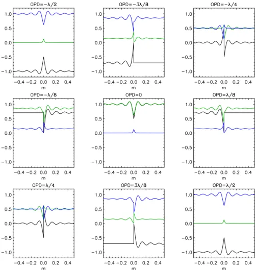
3.2.2. Behaviour of the MZ signal when introducing an OPD... 50
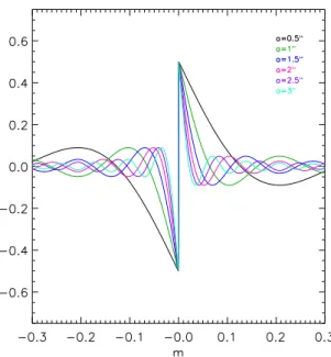
3.2.3. Behaviour of the MZ signal with pinhole size ... 52
3.3. Coronograph: a simplified approach to the Mach-Zehnder interferometer ... 54
3.4. Numerical Simulations... 57
3.4.1. Simulation of 1-D MZ signal ... 60
3.4.2. Aliasing effect ... 60
3.4.3. Influence of Turbulence on the MZ signal... 62
3.4.4. Influence of Gaps on the MZ signal... 66
3.4.5. Influence of the edge defects on the MZ signal ... 67
Contents
3.4.7. Multi-wavelength measurement... 76
3.4.8. Tip-Tilt considerations ... 78
3.5. Performance of a Mach-Zehnder co-phasing sensor... 81
3.5.1. MZ co-phasing sensor performance as a function of atmospheric turbulence. 83 3.5.2. MZ co-phasing sensor performance as a function of gaps... 86
3.5.3. MZ co-phasing sensor performance as a function of edge defects ... 88
3.5.4. MZ co-phasing sensor performance as a function of photon noise... 91
3.6. Summary ... 96
Chapter 4 Laboratory test of the Mach-Zehnder co-phasing technique... 99
4.1. Optical design for testing the MZ co-phasing technique ... 100
4.1.1. Segment Simulator ... 103
4.1.2. Turbulence Simulator... 105
4.1.3. Mach-Zehnder interferometer layout ... 107
4.2. Analysis of the experimental results ... 109
4.2.1. Performance without atmosphere... 112
4.2.2. Performance with atmosphere... 115
4.3. Summary ... 118
Chapter 5 Comparison of co-phasing techniques ... 121
5.1. Signal Characterisation ... 122
5.1.1. Sensibility to atmosphere, gaps and edge defects ... 123
5.2. Piston Retrieval ... 125
5.2.1. Precision, Capture Range and limiting magnitude... 125
5.2.2. APE the Active Phase Experiment... 127
5.3. Practical and Manufacturing considerations ... 128
5.4. Summary ... 131
Chapter 6 Conclusions and Perspectives... 137
ANNEX ... 139
Bibliography ... 143
List of Figures and Tables... 151
List of Acronyms
AO Adaptive Optics
APE Active Phase Experiment CIR Central Intensity Ratio
CMBR Cosmic Microwave Background Radiation CMOS Complementary Metal Oxide Semiconductor DFS Dispersed Fringe Sensor
ELT Extremely Large Telescope ESO European Southern Observatory FFT Fast Fourier Transform
FOV Field of View
FWHM Full Width Half Maximum
GF Grid Function
INAF Instituto Nazionale di Astrofisica
LAM Laboratoire d’Astrophysique de Marseille MCAO Multi Conjugated Adaptive Optics
MZ Mach-Zehnder
OPD Optical Path Difference
OPTICON Optical Infrared Coordination Network OTF Optical Transfer Function
PSF Point Spread Function
PtV Peak to Valley
RMS Root Mean Square
SNR Signal to Noise Ratio
List of Telescope Abbreviations
List of Telescope Abbreviations
CELT California Extremely Large Telescope
CFGT Chinese Future Giant Telescope
GTC Gran Telescopio de Canarias GMT Giant Magellan Telescope
GSMT Giant Segmented Mirror Telescope HDRT High Dynamic Range Telescope HET Hobby-Eberly Telescope JWST James Webb Space Telescope
LAMOST Large Aperture Multi-Object Spectroscopic Telescope LBT Large Binocular Telescope
LPT Large Petal Telescope
SALT Southern African Large Telescope TIM Mexican Infrared-Optical Telescope TMT Thirty Meter Telescope
VLT Very Large Telescope VLOT Very Large Optical Telescope OWL Overwhelmingly Large Telescope
Chapitre 1-Resumé
Les télescopes de prochaine génération repousseront les frontières des connaissances astrophysiques et seront la clef pour répondre à de nombreuses questions astrophysiques non résolues. Par exemple, la combinaison de la sensibilité et du champ fournis par les futurs ELTs permettra d’étudier l’évolution des grandes structures de l’univers, tandis que la combinaison de la haute résolution angulaire et de la très grande qualité optique devrait permettre de trouver des exoplanètes du type tellurique.
Bien que de grands miroirs monolithiques puissent être construits, la complexité de fabrication et le coût augmentent avec la taille. L’approche la plus réaliste pour les ELTs semble donc être l’utilisation de la segmentation.
Au cours des vingt dernières années, de gros efforts ont été faits dans le but d’améliorer la qualité des images des télescopes. Ces efforts se sont focalisés sur la correction des erreurs de front d’onde par l’amélioration de la qualité optique des télescopes ainsi que par l’introduction de l’optique adaptative corrigeant les perturbations atmosphériques. La qualité de l’image sera également affectée par la segmentation. L’espace entre les segments, les aberrations intrinsèques des segments, les erreurs de bords rabattus et les erreurs de piston et basculement (tip-tilt) provoquent de nouveaux effets de diffraction qui sont qualitativement et quantitativement différents selon la taille et le nombre de segments.
Nous décrivons brièvement les effets des erreurs de front d’onde sur la qualité des images, en portant une attention particulière à ceux causés par le mauvais alignement des segments.
Chapter 1
ELTs: Motivation and Description
In the next decades, astronomy will profit from a diverse set of observing capabilities, covering a broad range of wavelengths, on the ground and in the space. Two main reasons make the development of large ground based telescopes critical to expand astrophysical knowledge. First, the possibility of observing in a range covering from the optical to the infrared. Second, ground based facilities can deploy much more complex instrumentation than spaced-based missions.
Three broad topics are proposed by the Astrophysical Community: Cosmology, Galaxies, and Planetary Systems and Stars. Scientific cases will benefit from the wide capabilities of large telescopes, including sensitivity, wavelength coverage, field of view (FOV), spectral resolution, photometric and astrometric accuracy, high image quality and stability. We briefly describe some scientific cases including the required capabilities and instrumentation to carry out those programs.
A number of Extremely Large Telescopes (ELT) projects are currently in phase of design study. They differ mainly in the primary mirror selection, although segmentation is the common solution adopted in every case. We describe the different approaches proposed by the most important ELT projects.
The image quality is affected by segmentation. This chapter includes a brief description of the effects induced by wavefront errors on the image quality, with special attention to the effect of segmentation misalignment.
The role of ELTs in Astronomy
1.1. The role of ELTs in Astronomy
The enormous capabilities of the next generation of telescopes will expand the frontiers of astrophysical knowledge and will be the key to answer many unresolved questions. As a consequence, a large number of scientific cases have been proposed for ELTs, covering different astrophysical contexts ranging from our own Solar System to the very early epochs of the Universe. The European Astrophysical community, under the auspices of the OPTICON (Optical Infrared Coordination Network), has classified these different scientific cases into three main categories: Cosmology, Stars and Galaxies, and Planetary Systems and
Stars. We briefly present some of these science highlights that motivate and encourage the
development of ELTs.
In the coming decades, one of the most important challenges of observational cosmology will be to measure the evolution of the spatial distribution and properties of the baryonic content of the Universe in its different phases: galaxies and intergalactic gas. Establishing the statistical evolution of galaxies from their epoch of formation (more than 13 Giga-light-years away) to the present day, requires taking hundreds of high-resolution spectra (R>5000) of very faint objects (typically >25 AB mag) over a wide area (FOV ~ 5').
At the same time, mapping the 3-dimensional distribution of the cosmic gas in the Universe requires the acquisition of high quality spectra of faint objects in the distant universe, numerous enough to finely sample the large observed areas (FOV ~ 5'). These observations are necessary to discriminate among the competing theories at stake today. Their requirements call for ELTs, which have high enough sensitivity and FOVs. The Figure 1.1.1 shows an example of simulated distribution of cosmic gas at z=2.
Stars are one of the main components of galaxies, therefore it is of critical importance to understand how they form and evolve. With ELTs, stars of mass comparable to the Sun may be resolved in the outskirts of galaxies as far as the Virgo cluster (the closest cluster to the Milky Way). Reaching the Virgo cluster is important since it hosts a significant population of elliptical galaxies at the same distance and spanning a large range of magnitudes. With a very high spatial resolution (~10mas), required to diminish the effect of crowding, and a collecting power capable to reach typical magnitudes of ~35 in the optical band, we will be able to define the turn-off point of the color-magnitude diagrams of the studied stellar populations.
Figure 1.1.2 shows three color-magnitude diagrams for M32. As can be seen, the increases of the telescope aperture will result in better quality results for this kind of studies.
Figure 1.1.1 Projected neutral hydrogen in a simulation for z=2, from Katz et al (1996). The simulation box is
22.22 co-moving Mpc across, which corresponds to 7.4 physical Mpc at this redshift. For the CDM cosmology used, this translates into 15.1 arcmin.
Figure 1.1.2 Stellar populations at the center of M32. Left: Color-magnitude diagram of the central 30" of M32,
as observed with Gemini+Hokupa'a (Davidge et al. 2000). Middle: JWST color-magnitude diagram from a simulation assuming physical conditions similar to those of the center of M32. Right: GMST simulated color-magnitude diagram of the center of M32.
The discovery of extra-solar planets has placed our solar system in a new context and has revived the theoretical investigations of the formation and evolution of planetary system. These theories can be tested directly by measuring the gas phase dynamics and the chemical structure of protoplanetary disks. For this program high spatial (<80mas) and spectral (R~105) resolutions at thermal infrared wavelengths are required.
The role of ELTs in Astronomy
According to the scientific programs, the required capabilities can be gathered in four different operation modes:
i) Wide Field Mode: In this mode the angular resolution is limited by atmospheric conditions. It provides high sensitivity over a large FOV (~5’-10’).
ii) Classical Adaptive Optics Mode: This mode will provide diffraction-limited FOV around 10” in the infrared.
iii) Multi Conjugate Adaptive Optics (MCAO) Mode: MCAO (Beckers 1988) permits the extension of the diffraction-limited FOV beyond the limits of the isoplanatic patch. Moderate image quality can be reached over FOV of 30” in the visible and 2’ in the infrared.
iv) Extreme Adaptive Optic Mode: This mode provides diffraction limited images with very high quality but in small FOV (~1”-10”). The high spatial resolution and IR sensitivity of an ELT enables one of the most attractive and high priority targets of ELTs: to find the Earth like extra-solar planets around nearby bright stars.
1.2. ELT Projects
The technology developed for 10-m class telescopes serves as starting point for the design study of ELTs. In the current generation of large telescopes, two concepts primary mirrors have been pursued: monolithic mirrors and segmented mirrors.
Two technologies have been developed for current monolithic mirrors. The first one is the construction of a single large mirror made from borosilicate glass, but having large hollowed out regions to keep the weight down. This borosilicate honeycomb design has been pioneered by Angel & Hill (1982) and it has been successfully cast in the two 8.4-m primary mirrors of the Large Binocular Telescope (Hill & Salinari 2003). The second design is the thin mirror approach, primarily built by two companies, Corning (USA) and Schott (Germany). They used materials with good thermal properties, ULE (Corning) and Zerodur (Schott). Thin mirrors are being used for the four 8-m Very Large Telescope (VLT White Book, 1998). Although somewhat larger monolithic mirrors could be made, manufacturing complexity and relative cost increase with size. Therefore, the most realistic approach that can be extended to the ELTs involves the use of segmentation.
The feasibility of making segmented mirrors was first demonstrated by the Multiple Mirror Telescope (MMT) (Beckers et al, 1981) and TEMOS (Lemaître&Wang, 1993). The MMT was composed of six identical 1.8-meter telescopes in a single altitude-azimut mount. By contrast the TEMOS concept uses a primary mirror composed of large circular segments and a monolithic active secondary (Baranne&Lemaitre, 1987).
Three large segmented-mirror telescopes already exist: Keck I, Keck II (Nelson et al 1985)— which are two 10-m class telescopes composed by 36 hexagonal segments of 0.9m side— and the Hobby-Eberly Telescope (HET, Krabbendam et al 1998)- which is a 9-m telescope composed of 91 segments, each of 0.6 m side. Several others are being developed or have been proposed, including: Gran Telescopio de Canarias (GTC, Castro et al 2000) which has a similar configuration to Keck and the Southern African Large Telescope (SALT, Meiring et al 2003), whose design is based on HET. The Mexican Infrared-Optical Telescope (TIM, Cruz-Gonzalez, 2003), is a 8-m segmented telescope with 19 hexagonal segments with a maximum diameter of 1.8m. A very interesting project is the Large Aperture Multi-Object Spectroscopic Telescope (LAMOST, Wang et al 1996), which is a Schmidt telescope with a 5 degree FOV and active optics. The 6-m spherical primary mirror consists of 37 hexagonal
ELT Projects
spherical mirrors, each of them having a diagonal of 1.1m and a thickness of 75mm. The reflecting corrector of 4.5-m is located at the center of curvature of the primary mirror, it consists of 24 hexagonal plane submirrors, each of them having a diagonal of 1.1m and a thickness of 25mm. The available large focal plane of 1.75 meters in diameter may accommodate up to 4000 fibers, by which the collected light of distant and faint celestial objects down to 20.5 magnitude is fed into the spectrographs, which promises a very high spectrum acquiring rate of several ten-thousands of spectra per night.
ELT projects are currently in the concept study stage. The main discussions concerning the optical design turn on the choice of the primary mirror, which concerns the shape of the pupil, the size and shape of the segments and the density of the pupil, taken as the percentage of pupil filled with reflective surface.
The great advantage of spherical mirrors is their segment fabrication as all segments are identical. This option has been adopted for the 100-m project Overwhelmingly Large Telescope (OWL) due to the large number of segments to be fabricated, ~3000, with the consequent disadvantage of considerably increasing the complexity of the optical design in order to correct spherical aberrations.
Although the development of segmented mirrors dates from the last decade, there is still no agreement on the choice of the segment parameters. The Thirty Meter Telescope (TMT) proposed by an American-Canadian consortium opts for hexagonal segments of 0.5 to 1m side following the example of Keck. The uses of small segments reduce cost factors related to the fabrication equipment, transportation and coating chambers. It simplifies the support mechanism and it allows higher optical quality of the individual segment. On the other hand, the choice of large segments reduces the number of actuators and edge sensors required to control the shape of the mirror. At the same time it simplifies the telescope structure and reduces the edge sensor noise propagation. This alternative has been adopted for the 25-m Giant Magellan Telescope (GMT) and the 20-m Large Petal Telescope (LPT). The GMT used 6 circular segments while LPT employs 8 irregular hexagonal segments to fill a circular shape with a minimum of edges. The shape and size of the segments plays an important role on the diffraction effects observed in the focal plane. This aspect is of relevant importance since the diffraction effects can lead to confusion in the study of faint pointlike sources.
Table 1.2.1 Optical design for ELT projects.
Projects Optical Design M1
Diameter Number/size of segments F primary M2 Diameter LPT (Burgarella et al 2002) Ritchey-Chrètien /TMA1 20m 8 Petals 8m long F/1 5m HDRT (Kuhn et al 2001) Gregorian-TMA 22m 6 Circles 6.5m Diameter F/1 6m GMT (Angel et al 2004) Gregorian 25.3m 6 Circles 8.4m Diameter F/0.7 3.5m CFGT (Su et al 2004) Ritchey-Chrètien 30m 1122 Partial annular 0.8 m side F/1.2 2.1m VLOT (Roberts et al 2003) Ritchey-Chrètien 20m 150 Hexagons 0.9m side F/1 2.4m CELT (Nelson 2000) Ritchey-Chrétien 30m 1080 Hexagons 0.5m side F/1.5 3.96m TMT GSMT (Strom et al 2003) Cassegrian 30m 618 Hexagons 0.67m side F/1 2m Euro50 (Ardeberg et al 2000) Gregorian 50m 618 Hexagons 1.15m side F/0.85 4m OWL (Dierickx & Gilmozzi 2000) M1 Spherical M2 Flat 100m 3048 Hexagons 0.9m side F/1.25 34m
ELT Projects
Another parameter to be considered is the pupil density. The High Dynamic Range Telescope (HDRT) is a 22-m telescope formed by 6 off-axis, 6.5 m diameter, with a pupil density of 60%. By contrast, the Euro 50 —the 50-m telescope proposed by a consortium of European institutes— is a highly density pupil as the pupil is filled except for the obscuration due to the secondary.
In Table 1.2.1 we resume the main characteristics of the proposed ELTs. In most cases the secondary is monolithic except for OWL, where the huge size of the secondary implies its segmentation.
We remark the fast focal ratio of the primary to allow a compact telescope structure. This will make mirror manufacture harder.
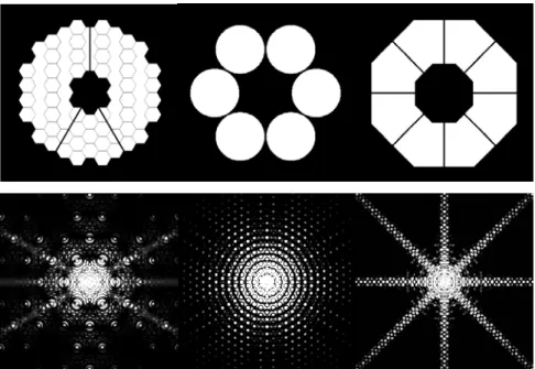
The primary mirror choice will play a fundamental role in the performance of diffraction images of point sources. Several simulation studies have been carried out in order to analyse the effect of segment size and shape on the image quality (Kuhn et al 2001, Marchis & Cuevas 1999). Zamkotsian et al (2003-2004) performed the comparison of the point-spread-function (PSF) for three different mirror approaches, as seen in Figure 1.2.1. They found particularly interesting the case of polygonal petals, because the number of diffraction spikes in the PSF is minimised leading to large areas of low levels of scattered light close to the core. This is important for high dynamic range imaging.
Figure 1.2.1 Three different segmentation concepts with hexagonal, circular and polygonal segments (upper
For certain scientific cases diffraction effects due to segment misalignment are not negligible. Diffraction effects from highly segmented mirrors have been studied in detail elsewhere (Zeider & Montgomery 1998, Troy & Chanan 2003, Yaitskova et al 2003, Bello et al, 2000), and we will briefly present them here.
Image quality of a highly segmented mirror
1.3. Image quality of a highly segmented mirror
In the last twenty years hard efforts have been concentrated in order to improve the image quality of telescopes. Those efforts are focused in the correction of wavefront errors introduced by the atmosphere, by the use of Adaptive Optic (AO) Systems, as well as the reduction of wavefront errors related to the telescope optic quality, by the use of Active Optic Systems. Image quality will also be affected by segmentation. Gaps, individual segment aberrations, edge miss-figure errors and piston and tip-tilt misalignments result in new diffraction effects which are qualitative and quantitatively different according to the size and segment number.
In this section we briefly describe the effect of segmentation on the image quality paying special attention to the effect of segmentation misalignments. We also describe the most important properties of atmosphere turbulence and its influence on the image quality.
1.3.1. Effect of segmentation on the image quality
Generally segments have six degrees of freedom: translation along two axes in the plane of the segment, rotation about a vertical axis, rotation about two horizontal axes (tip and tilt), and translation along the vertical axis (piston). Misalignments of the three first degrees of freedom are not critical for the image quality (Mast 1982). However, movement of pistons or tip-tilts produce wavefront discontinuities which damage the image quality.
In order to quantify the quality of the image, several criteria are used. Yaitskova et al (2003), employ peak intensity and mean halo intensity of the PSF. Diericks (1992) proposed the Central Intensity Ratio (CIR), defined as the ratio between the central intensity given by the telescope divided by the central intensity given by an equivalent perfect telescope without aberrations but under the same seeing conditions. We limit this discussion to the Strehl ratio, a criteria frequently employed in astronomy. It is equal to the ratio between the central intensity of the aberrated PSF and the central intensity of the diffraction-limited PSF.
The PSF of a segmented telescope can be represented by (Yaitskova et al 2003),
2 s PSF( ) AN GF( )PSF ( ) z λ = w w w (1.1)
where A is the segment area, N is the number of segments, λ is the wavelength and z is the focal distance. GF(w) and PSFs(w) are two functions which depend on the geometry of the
telescope segments. The function GF(w) is the Fourier Transform of the segmentation grid, usually a periodic array of peaks of width inversely proportional to the diameter of the full aperture. The PSFs(w) is the PSF of an individual segment, whose width is inversely
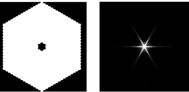
proportional to the segment size. In Figure 1.3.1 we have plotted the PSF of a 50m telescope with 714 segments, supposing that the telescope is completely phased with perfect segments and no gaps between them. In this case, zeros of the segment PSF coincide with the peaks of the GF term, so that only the central peak is observed. The six diffraction arms are the result of the hexagonal shape of the telescope pupil.
Figure 1.3.1 Pupil of a 50m class segmented telescope with 714 segments without any error (left) and its
corresponding PSF(right).
The presence of piston will not influence the segment PSF. However, it will modify the grid term introducing a noisy speckle background. In Figure 1.3.2, we represent a segmented pupil with piston RMS error equal to 120nm and its corresponding PSF over a field of 0.5”. The size of the speckle field is equal to the size of the segment PSF, and does not depend on the value of the piston error.
Assuming piston errors with Gaussian distribution and zero mean, the Strehl ratio of the PSF is given by; 2 1 1 ( 1) S N e N σ − = + − (1.2)
Image quality of a highly segmented mirror
where N is the number of segments and σ is the standard deviation of the phase error. For highly segmented mirrors and small errors, this result is consistent with the Marechal approximation; S~1-σ². For a 100m class telescope with around 3000 segments, the global piston RMS error at the wavefront should be less than λ/20 (25nm@500nm) in order to get a Strehl ratio of 90%. This implies that the co-phasing technique should be able to measure discontinuities of the order of λ/40 (12nm@500nm) in the mirror surface.
For high contrast imaging, it is very important to quantify the intensity lost from the central peak. This is mainly transmitted into a diffuse halo of speckles of width λ/d and can be
expressed as, 2 2 2 d I D πσ λ = (1.3)
For a 100-m telescope, using a wavelength of 500nm, the RMS error should be less than 1nm in order to reduce the halo intensity to 10-10. This implies an extreme co-phasing precision for high contrast imaging applications.
Figure 1.3.2 Segmented pupil with RMS piston error of 120nm (left) and its corresponding PSF (right).
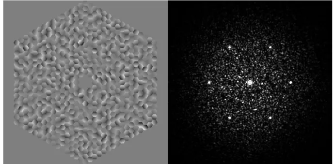
The effect of tip-tilt errors will modify the PSFs term of (1.1). For a small number of
segments and large tip-tilt errors the PSF is the composition of the shifted individual PSFs of segments. If tip-tilt error decreases; the peaks overlap each other forming an interference
pattern, which, in the limit of zero tip-tilt error, is the PSF of the whole mirror. By increasing the number of segments, the PSF is composed by a regular grid of spots of the same size of the telescope Airy disk, in addition to the appearance of a speckle background (see Figure 1.3.3). This regular structure coincides with the interference pattern from a random blazed two-dimensional (2-D) grating (Yaitskova & Dohlen 2002). The period of the regular grid of spots is inversely proportional to the separation between segments. The Strehl ratio for small tip-tilt error can be expressed as,
+ + − ≈ N S 2.34 2 4 1 σ2 σ4 (1.4)
Unlike the piston case, this expression is not strongly dependent on the number of segments. Once more, for a large number of segment and small errors the Marechal approximation is valid. To achieve a Strehl ratio of 90%, the global tip-tilt error in the wavefront should be less than λ/20 (25nm@500nm).
Figure 1.3.3 Segmented pupil with RMS tip-tilt error of 100nm (left) and its corresponding PSF (right).
Other error sources related to the quality of the individual segment will have similar effects on the PSF as tip-tilt errors. For example, edge defects lead to the appearance of secondary peaks and a background speckle field. Image quality performance in terms of Strehl ratio is
Image quality of a highly segmented mirror
not significantly reduced, 0.95 Strehl ratio is achieved for typical values of edge miss-figure of the order of 5 to 10 mm width and 200nm amplitude.
1.3.2. Influence of atmospheric turbulence on the image quality
Atmospheric turbulence is caused by spatially and temporally random fluctuation of the refraction index. Fluctuations in the refraction index, mainly on account of temperature variations, result in random spatial and temporal variations of the optical path length.
Kolmogorov (1961) developed a model in which the kinetic energy was transmitted successively from the largest scale motions to the smallest ones. He assumed that the motion of the small turbulent scale is homogeneous and isotropic, i.e. the statistical characteristic of the turbulent flow depends only on the distance between any two points on the structure. The statistical distribution and number of turbulent eddies with uniform diffraction index is characterized by the power spectrum of the refractive index fluctuation, Φn(k), being k the
spatial wavenumber related to the isotropic scale size l, as k=2π/l. Three different regimes are considered. The outer scale regime, when k< 2π/L0, being L0 the largest scale for the turbulent
motions of the order of tens of meters, in which Φn(k) depends on geographical and
meteorological conditions. The inner scale regime when k>2π/l0, being l0 the smallest size of
turbulent eddies of the order of millimetres.
The Kolmogorov spectrum in the regime between the outer and inner scale, can be expressed mathematically as (Noll 1976),
11/ 3 5/ 3 0 ( ) 0.023 k k r− k− Φ = (1.5)
where r0 is the Fried (Fried 1966) parameter given by,
3/ 5 2 0 2 0 cos 0.185 ( )d L n r C z z λ γ =
∫
(1.6)where γ is the angle of observation and 2( )
n
C z is the structure constant of the index of
refraction fluctuation which is a function of altitude, z. Experimental measurements have demonstrated that the structure function varies from site to site and also with time. The Fried parameter r0, it is the aperture over which there is approximately one radian RMS phase
aberration, and hence it is the maximum aperture bellow which diffraction limited resolution is possible. For example, a 10m telescope observing under turbulence conditions with
r0=10cm in the visible, will not obtain a better resolution than a 10cm telescope.
The Full Width Half Maximum (FWHM) of the atmospheric PSF is called Seeing (β). It is
the parameter most commonly used in astronomy to characterise atmospheric conditions and it is given by, 0 0.98 r λ β = (1.7)
To avoid the singularity of the Kolmogorov model for wavenumber close to zero an alternative model is proposed. It is known as von Karman model (Roggeman 1996), and the spectrum of the index fluctuation is given by,
5/ 3 2 0 2 2 11/ 6 2 0 0.0229 ( ) exp ( ) V n m r k k k k k − Φ = + (1.8)
where k0=2π/L0 and km=5.92/l0. Both models are coincident in the regime between outer and
inner scale.
Locally fluctuations of the refraction index cause phase variations on the wavefront, and propagation of a plane wave trough the turbulence introduces phase and amplitude variations. The temporal behaviour of the atmosphere is characterized by a correlation time, τ0,
0 0 0.31
r V
τ = (1.9)
where V is the mean wind speed.
Short exposure imaging refers to the situation in which exposure time is less than correlation time, τ0. This exposure time is short enough to freeze the speckle effects of
atmosphere, see Figure 1.3.4.
When the exposure time is much longer than the correlation time of atmosphere, the image is called long exposure image. In this case, atmosphere is averaged over a large number of independent realizations, given a broader and smoother PSF.
The optical transfer function (OTF) for long exposure images can be expressed as (Roggeman & Welsh 1996),
Image quality of a highly segmented mirror 5/ 3 LE 0 H ( ) T( ) exp 3.44 r λ = − f f f (1.10)
where T(f) is the OTF of the telescope. The simulated PSF for long exposures can be obtained from the Fourier transform of (1.10).
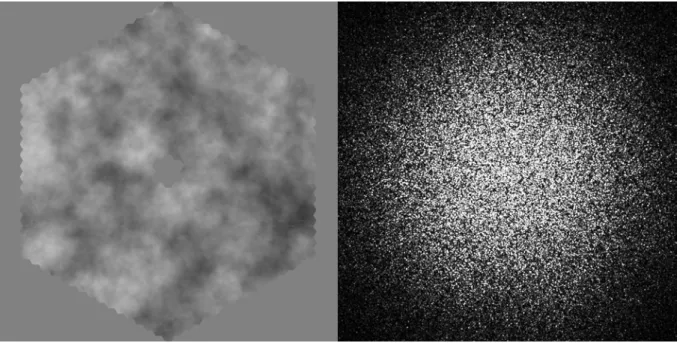
Figure 1.3.4 Simulated phase screen for 50m telescope, with r0=15cm (left), and its corresponding short
exposure PSF.
AO is able to compensate in real time wavefront errors introduced by atmosphere, thus restoring image quality.
As described in section 1.1, ELTs will operate in different modes depending on the scientific target. Therefore, image quality and the degree of correction will vary according to the scientific case.
Image quality will be improved in different stages. The first stage involves correcting misalignment errors between segments to obtain the desired shape of the primary mirror. The
co-phasing procedure should be able to detect piston errors of the order of tens of nm. This is
the aim of developing new co-phasing techniques described in the next section. This procedure must be carried out before scientific observations are made and, in principle, one iteration per night should be sufficient. Other scientific programs require higher image quality. AO systems enable wavefront corrections in real time with Strehl ratios of the order
of 50%. Up to now AO systems have been applied to correct high order aberrations. In the case of ELTs, discussions focus on the development of combined systems that will correct the whole range of frequency at the same time. One of the main difficulties of AO systems for ELTs is in its manufacturing. For example, the internal pupil diameter cannot be reduced below 1m for a 100m primary considering a 10 arcmin FOV (total FOV of OWL) and a maximal beam angle of 10° on the Deformable Mirror.
If the image quality has to be improved up to Strehl ratios higher than 90% with very high contrast —which will be the case of detection of extra-solar planets— Extreme AO corrections are required. Simulation results (Riccardi et al 2003) show that the co-phasing procedure precision should be above 1 nm in order to reduce the halo due to piston. This implies real time correction of segment misalignments. To this regard, Brusa et al (1999) proposed an adaptive primary mirror able to correct the ground layer and segment misalignments simultaneously. However, this question remains unresolved in obtaining the perfect telescope performance.
Chapitre 2-Resumé
Les grands télescopes sont équipés d’optique active dans le but de maintenir automatiquement la forme et la position requise du miroir. En effet, les effets gravitationnels et thermiques génèrent des variations de grandes amplitudes dans les systèmes optiques. D’autre part, ces variations étant quasi statiques (moins d’un Herz), une opération en boucle fermée est moins contraignante que dans le cas de l’optique adaptative.
La boucle de contrôle du co-phasage est schématiquement formée de trois éléments. Les capteurs de position situés derrière ou sur le côté de chaque segment fournissent en permanence les positions relatives entre 2 segments adjacents avec une précision de quelques nanomètres. Les actionneurs situés en dessous de chaque segment compensent les déplacements entre segments. Et finalement le capteur de co-phasage fournit les informations pour la calibration périodique du capteur de position, afin de permettre la mesure absolue du piston de chaque segment.
Nous présentons ici un état de l’art des différentes techniques de co-phasage. Nous incluons la plus connue des techniques, celle proposée par Chanan et al (1998) et déjà implémentée au télescope Keck. Nous décrivons également d’autres analyseurs de co-phasage basés sur la méthode de courbure, le principe à pyramide et l’interféromètre de Mach-Zehnder (MZ), qui sera le sujet de ce travail.
Chapter 2
Review of co-phasing Techniques
Large telescopes are equipped with active optics in order to automatically maintain the required shape and position of the mirror. Most errors in the optical setup are associated to gravity and temperature variations. Given that those variations are quasi static —less than 1 Hertz— the conditions for the close loop operation are relatively relaxed compared with those required for Adaptive Optic.
The co-phasing control loop is formed basically by three elements. The position sensors located at the back or at the edge of each segment permanently provide relative positions of two adjacent segments with a few nanometres accuracy. The actuators situated underneath each segment compensate displacements between segments. Finally, the phasing sensor provides information for periodical calibration of the position sensor to enable measuring absolute piston differences between segments.
Various co-phasing sensors are based on existing wavefront sensors usually employed in AO applications, for example Curvature, Shack-Hartman or Pyramid. Although the wavefront sensor setup does not suffer major changes, the wavefront sensor in the AO application detects continuous variations in the wavefront, either curvatures in the case of Curvature sensor or slopes in the case of Pyramid and Shack-Hartman sensors. However, for co-phasing applications the interest lies on measuring discontinuities on the wavefront. In this case, the recorder signal is the result of the diffraction effect propagation due to segmentation.
In order to achieve the best performance, the co-phasing technique must deal with additional wavefront errors, i.e. segment and edge miss-figure, atmospheric turbulence, gaps, cross-talk between contiguous edge, photon noise, propagation errors, etc. Some of the methods presented here are not suitable for ground based telescopes since they do not include atmospheric errors. This is the case, for example, of the co-phasing technique described for James Webb Space Telescope, JWST (Seery 2003).
Diffraction co-phasing techniques
2.1. Diffraction co-phasing techniques
Diffractive techniques are based on the analysis of images produced by a lenslet array situated in the conjugate plane of the telescope pupil.
The Phasing Camera System described by Chanan et al (1998), currently operating at the Keck telescope, is a diffractive wavefront sensor in which the lenslet array is preceded by a mask at the position of the exit pupil. The mask defines a small circular subaperture of 12cm in diameter (referred to the primary) at the center of each intersegment edge. The size of the subapertures is small in comparison with the Fried parameter —of the order of 20cm— so as to ensure low dependence on atmospheric turbulence. Piston information is contained in the diffraction pattern of each subaperture. Piston is obtained from the correlation of the measured image with a simulated set of templates. In the Narrow–Band regime (Chanan et al 2000) images are cross-correlated with a set of 11 templates in the range of half a wave. The capture range of this technique can be increased by using multiple wavelengths.
In the Broadband regime (Chanan et al 1998), a set of 11 templates are simulated in the range of the coherence length of light. The step is obtained from the “coherence parameter”, defined as the difference between maximum and minimum correlation coefficient.
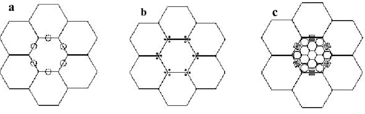
Korhonen & Haarala (1998) proposed a procedure which is similar to Chanan with three subapertures at the corner of the segment mask as shown in Figure 2.1.1.
Figure 2.1.1 Masks for the Shack Hartman sensor proposed by; a: Chanan et al (1998); b: Korhonen & Haraala
(1998), and c: Bello-Figueroa (2001).
Bello-Figueroa (2001) proposed a modification of the Chanan technique for the GTC telescope. The geometry of the mask, proposed for the GTC acquisition camera, allows one to
measure segment discontinuities as well as segment figure errors. They replaced the circular aperture used for Keck with a double slit. This way the effect of edge miss-figure can be avoided, as seen in Figure 2.1.1. The algorithm used to retrieve step errors is based on the properties of the diffracted image. Figure 2.1.2 shows a set of diffraction images and the vertical profile for different piston errors. A calibration curve is obtained from the difference between the two main peaks of the diffraction pattern. For a given diffracted image, the peak ratio is calculated and processed by the calibration data in order to obtain the required piston step.
Schumacher et al (2002) improved and completed the GTC study for the case of ELTs. Firstly, they fitted the diffraction images using a double Gaussian model which allows them to get a more accurate measurement of the peak difference, even under turbulence conditions. Secondly, they used weightings on individual measurement errors when the piston values of all segments were calculated by Single Value Decomposition (SVD), a standard method to find the least-squares solution to an over determined set of linear equations (Press et al 1992).
Figure 2.1.2 Simulated 2-D diffraction pattern (left) and the x-projection (right) of a double slit for 0, upper left
Co-phasing techniques based on Curvature sensors
2.2. Co-phasing techniques based on Curvature sensors
The Curvature sensor introduced by Roddier & Roddier (1993) for AO is presented in Figure 2.2.1. Two detectors placed at equal distance, l, in front and behind the focal plane measure the intensity distribution in both planes. There is a local excess of illumination in one plane and a lack of illumination in the other as a result of the local curvature in the wavefront.Figure 2.2.1 Principle of Curvature wavefront sensor (from Schumacher & Devaney,2004).
Roddier & Roddier define a quantity denominated Curvature Signal, which in the near– field approximation, is equal to,
2 e i c e i I I W CS z P W I I δ − ∂ = = ∆ − ∇ + ∂n (2.1)
where Ie and Ii are the extra and intra focal intensity distribution at the image plane, ∆z is the
defocused term which depends on the focal length f and on the defocused distance l with respect to the focal plane as ±f(f-l)/l; W is the wavefront; P is a function equal to 1 inside the pupil and 0 outside; n is an unitary vector pointing outside the pupil and δc is a linear Dirac
distribution around the pupil edge.
The first term in parentheses is proportional to the variation of the wavefront at the pupil edge and the second term is the wavefront Laplacian across the beam, which is proportional to the curvature of the wavefront.
Roddier assumed continuity of wavefront phase function in his mathematical description of this method. This can not be assumed in a segmented telescope, thus the term “Curvature
sensor” is not strictly appropriated to appoint a group of co-phasing techniques. Nevertheless, it is useful as a reference to a well known instrumental technique.
In the presence of phase discontinuities, the signal can be simulated using Fresnel diffraction theory. The complex amplitude in the output pupil is given by,
2 ( ) ( ) exp ( ) d 2 jk z zF e k u U j jk z z ∞ ∆ −∞ = − ∆
∫ ∫
∆ x x' x x' x' (2.2)where, U(x’) is the complex input amplitude, k is the wave number 2π/λ and ∆z is the defocus
term. The Fresnel approximation is valid when the defocus term ∆z is much larger than the segment size.
The Fresnel integral can be considered as the convolution of the complex input amplitude
with a function containing the defocused term. Since the convolution is a multiplication in the frequency domain, the complex output amplitude is simulated with FFT algorithms as;
(
)
1 2 , exp( ) ( ) ( ') exp ' 2 z F ik z ik u FFT FFT U FFT ik z z − ∆ = ∆ ∆ x x x (2.3)Figure 2.2.2 shows an intra focal image and the Curvature signal for a 50 m segmented telescope with random piston error of 100nm. Piston errors appear as a modulation of intensity at the edge of the segments.
Figure 2.2.2 Intra focal image (left) and curvature signal (right) of a 30m telescope, with a defocused distance of
Co-phasing techniques based on Curvature sensors
The signal changes in the direction perpendicular to the border while it remains constant along the edge direction. The signal width depends on the pupil defocused distance; ∆z, small
pupil defocused distance —thus large l— leads to narrower signal.
Rodriguez-Ramos & Fuensalida (1997) first proposed to use the Curvature sensor to measure piston errors. They proposed an iterative technique which compared the measured curvature with the simulated curvature signal of an array of segments with known piston errors. This technique fails when seeing is included. They also proposed a hybrid sensor, which includes a Shack-Hartman sensor to correct turbulence errors.
Chanan et al (1999) proposed a method which is similar to the previous one. In this method defocused pairs of images of each segment were simulated, and experimental images were correlated with the simulated templates. Measurements were done for λ=3.3µm for two main reasons, i) it decreases influence of atmosphere, and ii) it keeps defocus distance in the Fresnel approximation. For perfect segment shape they achieved a precision of 5nm and a repeatability of 40nm.
Cuevas et al (2000) proposed a generalisation of the Roddier equation including discontinuity errors, based on the distribution theory. They argued that piston step is proportional to the amplitude of the first derivative of the linear Dirac delta distribution, and tip-tilt is proportional to the amplitude of the Dirac delta distribution. This generalisation is only valid if the signal width is close to zero, which is the case of weak defocused pupils. Rodríguez-González & Fuensalida (2003) developed an analytical model based on the diffraction phenomenon of propagation. This model describes curvature signal including wavefront discontinuities. From Fresnel propagation theory they deduced the expressions of the curvature signal for a square aperture with segmentation discontinuities. The signal was characterised as a function of sensor parameters, i.e. focal length, defocus distance, wavelength, etc. They developed a model in order to retrieve piston errors by defining an integrated curvature signal for each segment. This way, it was possible to reduce the number of measurements to the number of segments, and therefore they managed to decrease time consuming and computer memory requirements. From simulations, they obtained a precision of 69nm for λ=600nm, 48nm for λ=1.2µm and 13nm for λ=2.4µm. However, the algorithm needs to be completed with the inclusion of atmospheric errors.
2.3. Other alternatives for co-phasing
Another set of techniques is based in the phase diversity principle proposed by Gonsalves & Chidlaw (1979). The pupil aberrations are calculated from the simultaneous measurements of a focused and a slightly defocused image. Lofdahl et al (1998) performed an experiment at Keck II telescope which involved measuring a large number of pairs of images. The average of the individual result gave the misalignment measurement. However, the results obtained in this experiment were not satisfactory, probably due to the poor seeing conditions in which this experiment was carried out.
Phase diversity has been also proposed by Baron et al (2003) for co-phasing of multi-aperture arrays using extended sources. The performance of the phase diversity algorithm is severally affected by the redundancy and dilution of the sub-apertures. Sorrente et al (2004) experimentally tested the validity of this technique obtaining consistent results with numerical simulations.
Labeyrie et al (2002) proposed an alternative method for co-phasing multi-aperture arrays —particularly applicable to hypertelescopes with a densified pupil (Labeyrie 1996) — based on the dispersed-speckle methods. This technique exploits the chromatic dependence of speckled images. It was demonstrated that the wavelength-dependent three-dimensional (3-D) complex input amplitude is the 3-D Fourier Transform of the cube data formed of speckled images at different wavelengths. The piston step map was reconstructed by a 3-D Fineup algorithm.
The JWST would require a co-phasing procedure with the advantage of avoiding atmospheric effects, unlike ground based telescopes. The phasing protocol combines two co-sensing techniques: i) The Dispersed Fringe Sensor (DFS) provides a robust phasing signal over about 1 µm of piston error. It uses a transmissive grism which spreads the light according to its wavelength, forming a spectrum on the camera. Piston differences are measured from the intensity modulations on the spectrum (Shi et al 2003); ii) White Light Interferometry (WLI) provides more than tens of nanometres of precision. Each segment is pistoned over a range which depends on the filter width. The broadband PSF corresponding to each piston position is recorded. The relation of the intensity of the central pixel of the PSF versus the piston position is the WLI signal for that segment (Shi et al 2003).
Pyramid sensor for measuring dephased errors
2.4. Pyramid sensor for measuring dephased errors
The concept of the Pyramid wavefront sensor is based on the principle of the knife edge test (Foucault 1859) introduced by Ragazzoni (1996) for AO, see Figure 2.4.1. A glass pyramid is placed in the focal plane of the telescope, so that each side of the pyramid acts as a spatial filter, producing four different images of the pupil in the observation plane. The combination of the intensity distribution over the four quadrants is proportional to the local slopes of the wavefront, assuming geometrical approximation. By introducing a modulation on the wavefront tilt, the sensitivity and dynamic range of the sensor can be tuned. Small modulation amplitude provides better sensitivity in order to measure small wavefront aberration, while large modulation leads to larger dynamic range with less precision when measuring large aberrations.
Figure 2.4.1 Scheme of a Pyramid wavefront sensor. Figure taken from Esposito (2000).
Modulation can be introduced either i) dynamically, by moving the pyramid or placing an oscillating tip-tilt mirror in the exit pupil conjugate plate, or ii) statically, by placing a diffusing element in an intermediate image of the pupil (Ragazzoni et al 2002).
Esposito & Devaney (2002) proposed a method for co-phasing segmented mirrors using a Pyramid wavefront sensor. Although in the geometric optics regime the Pyramid Sensor detects local wavefront tilts, diffraction of wavefront discontinuities give rise to a signal in the Pyramid sensor which can be used to measure piston. The optical configuration is the same but the tip-tilt modulation is no longer required. The amplitude of the signal is a sinusoidal function of the piston step. The sensor has the ability to measure misalignment of the segments and wavefront aberrations simultaneously.
2.5. Interferometric techniques for co-phasing segmented
mirrors
Interferometric techniques measure piston errors by analysing the interference pattern produced either in a plane conjugated to the primary mirror or locally, at the intersegment zone. There are many ways of implementing interferometic techniques for co-phasing applications. The interferometric techniques presented here can be classified according to the type of source employed, either artificial or natural. They differ firstly in the interferometric technique they adopt, which can be mainly Michelson, Shearing or Mach-Zehnder (MZ) interferometers, and secondly in the optical configuration in relation to the interferometer location, sometimes in the centre of curvature others in the focal plane. We next expose some examples.
Figure 2.5.1 3-D layout interferometer proposed by Pizarro. Figure taken from Pizarro et al. (2002).
Pizarro et al (2002) proposed to measure piston errors using a Michelson interferometer mounted on a robotic arm which position the interferometer in front of the segment edges, as shown in Figure 2.5.1. There is an internal light source which illuminates the segments, the reference beam reflected from one segment interferes with the beam reflected from intersegment region. Piston errors cause mismatching of the fringes from each side of the edge segment. Relative segment tilt causes the fringe period to change and relative segment tip causes the fringes to deviate from the vertical. The position of zero piston error can be
Interferometric techniques for co-phasing segmented mirrors
narrowband light to give several fringes. The main advantage of this method is that the co-phasing is done during day time. Experimental measurements (Pinto et al 2004) show that a precision of 5nm with a range of 30µm is achieved.
Kishner (1991) proposed measuring absolute distances with an interferometer placed in the centre of curvature of the primary mirror, as seen in Figure 2.5.2. Reflectors components were positioned on the segment surface. Interferences formed between the reference beam and the beam coming from the reflecting points. This method allows them to measure both, misalignment errors and aberrations of the segment surface depending on the number of reflectors placed onto the segment. This method is very sensitive to the fluctuation on the refractive index thus to the atmospheric turbulence.
Figure 2.5.2 Sample point interferometer proposed by Kishner. Figure taken from Kishner (1991).
Voitsekovich et al (2002) proposed an approach based in a shearing interferometer with a simple setup composed of two lenses and a filter between them, which provides not only relative piston information but also information on relative tilt and defocus. Intensity distribution on the image plane is formed by a central interference pattern produced by to adjacent segments, enclosed by the direct field and shifted field of the surroundings segments. They provide a description of the filter design and manufacturing. The reconstruction of the piston map error requires to measure two interferograms using two different filter orientations. This method has a maximum precision of λ/45 at the wavefront, when a significant noise level is considered. When atmospheric errors are considered, the distance
between the interference points (~1m) is much bigger than r0 (~0.25m), therefore the phase
fluctuations are de-correlated and the interferogram is blurred by atmosphere.
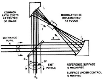
Horton et al (1990) used a radial shearing interferometer as shown in Figure 2.5.3. Two images of the segment pupil with different magnification will interfere producing a fringe pattern in the exit pupil. A rotating tilted transparent plate situated in the focal plane modulates the tilt fringes used for sampling the segment misalignment.
Figure 2.5.3 Shearing interferometer proposed by Horton et al. Figure taken from Horton et al (1990).
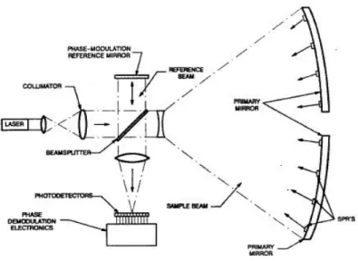
Dohlen & Fresneau (2000) proposed a dual wavelength random phase shift interferometer for phasing segmented mirrors using an artificial source located at the centre of curvature of the primary. They suggested the implementation of this technique for stellar sensors using a MZ interferometer, as proposed by Angel (1994) for high precision AO.
This principle was later elaborated by Montoya et al (2002) and its description is the subject of this work.
Chapitre 3-Resumé
Une nouvelle technique de co-phasage des miroirs segmentés, basée sur l’interféromètre de MZ, est présentée dans ce chapitre. Dans un interféromètre de MZ, une lame séparatrice divise le faisceau provenant du télescope en deux bras. Un trou placé au plan focal d’un des bras agit comme filtre spatial, fournissant une onde de référence cohérente avec l’onde entrante. Si la taille du trou est plus grande que la tache d’Airy, l’onde de référence contient les composantes basse fréquence de l’onde objet.Après réflexion sur les miroirs plans, les faisceaux filtrés et non filtrés sont recombinés par une lame séparatrice, formant deux interférogrammes complémentaires. Ces interférogrammes contiennent seulement les hautes fréquences du front d’onde entrant, éliminant ainsi les perturbations atmosphériques et ne laissant que les erreurs de segmentation.
Nous avons réalisé une étude analytique des interférogrammes de MZ pour le cas mono-dimensionnel avec des erreurs de piston. Des analyses complémentaires de ces interférogrammes utilisant des simulations numériques montrent un bon accord avec les résultats analytiques.
Nous avons décrit plusieurs algorithmes pour retrouver les erreurs de front d’onde causées par la segmentation, et nous avons étudié leurs précisions lorsqu’on inclut non seulement les erreurs de discontinuité mais également la turbulence atmosphérique et les erreurs causées par les bords rabattus. En changeant la taille du trou, les performances en tenant compte des erreurs atmosphériques peuvent être optimisées. Plus critiques sont les effets de bords rabattus produits durant la procédure de polissage. Cependant, une précision de 10nm peut être atteinte dans tous les cas.
La technique du MZ employant la lumière d’une étoile naturelle, il est important de déterminer l’influence du bruit de photon sur les performances de cette méthode. Les conditions requises concernant la magnitude limite de l’étoile ne sont pas très drastiques puisqu’une étoile plus brillante que la magnitude 14 en bande V suffira pour assurer une précision de 10nm.
Chapter 3
Mach-Zehnder co-phasing technique
In this chapter we introduce a novel technique for co-phasing of segmented mirrors based on a MZ interferometer. We present a general description of this method, in which we justify the use of a MZ interferometer for measuring wavefront discontinuities.
We have performed an analytical study of the MZ interferograms for the one-dimensional (1-D) case for pure piston error. Further analysis of the MZ interferograms using numerical simulations shows a good agreement between the results of both, analytical and numerical approaches. We also present a coronograph approach as an alternative instrument based in the same principle as the MZ technique.
Finally, different algorithms to retrieve wavefront errors are described. We report on the precision obtained when including not only discontinuity errors but also atmospheric turbulence and edge defects. The detection parameters and photon noise have been also implemented in the simulation. Our analysis resulted in an optimal configuration achieving the highest performance of the instrument.
General Description
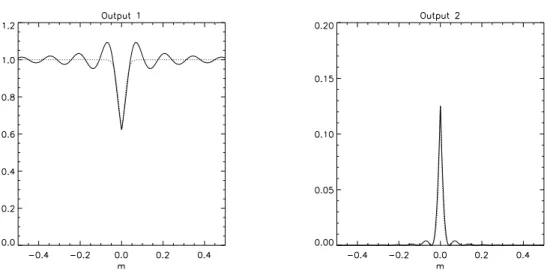
3.1. General Description
The purpose of a MZ wavefront sensor is to measure phase properties of the incoming wavefront by applying the appropriate spatial filtering in one of the interferometer arms. The idea of using this kind of interferometer to measure atmospheric wavefront errors was first introduced by Angel (1994). A scheme of the MZ interferometer is shown in Figure 3.1.1.
Telescope focus Pinhole Interferogram Interferogram Reference channel Beamsplitter Beamsplitter UA UB A1, ϕ1 A2, ϕ2
Figure 3.1.1 Scheme of a MZ interferometer.
In MZ interferometer, a beam splitter divides the incoming beam from the telescope focus. A pinhole placed in the focal plane of one arm acts as a spatial filter, providing the reference wave coherent to the incoming wave. After reflection at plane mirrors, the two beams are recombined by a second beam splitter, forming two complementary interference patterns. If the pinhole size is smaller than the Airy disk, the reference beam is a spherical wave. In this case the difference of intensity between two interferograms directly provides the local phase. On the contrary, if the pinhole size is larger than the Airy disk, the reference wave contains the low frequency components of the object wave. At recombination, as result of the subtraction of the two wavefront arms, the interferograms contain only the high frequencies of the incoming wave.