HAL Id: hal-01270963
https://hal.archives-ouvertes.fr/hal-01270963
Submitted on 8 Feb 2016
HAL is a multi-disciplinary open access
archive for the deposit and dissemination of sci-entific research documents, whether they are pub-lished or not. The documents may come from
L’archive ouverte pluridisciplinaire HAL, est destinée au dépôt et à la diffusion de documents scientifiques de niveau recherche, publiés ou non, émanant des établissements d’enseignement et de
On combining wavelets expansion and sparse linear
models for Regression on metabolomic data and
biomarker selection
Nathalie Vialaneix, Noslen Hernández, Alain Paris, Céline Domange, Nathalie
Priymenko, Philippe Besse
To cite this version:
Nathalie Vialaneix, Noslen Hernández, Alain Paris, Céline Domange, Nathalie Priymenko, et al.. On combining wavelets expansion and sparse linear models for Regression on metabolomic data and biomarker selection. Communications in Statistics - Simulation and Computation, Taylor & Francis, 2016, 45 (1), pp.282-298. �10.1080/03610918.2013.862273�. �hal-01270963�
On combining wavelets expansion and sparse
linear models for regression on metabolomic
data and biomarker selection
Nathalie Villa-Vialaneix
1,2∗, Noslen Hern´andez
3, Alain Paris
4,
C´eline Domange
5,6, Nathalie Priymenko
7, Philippe Besse
81 SAMM, Universit´e Paris 1, 90 rue de Tolbiac, F-75013 Paris - France 2 Universit´e de Perpignan Via Domitia, IUT, Dpt STID, F-66860 Perpignan - France
3 Advanced Technologies Application Center, CENATAV, Havana - Cuba 4 INRA, Unit´e M´et@risk, AgroParisTech, 16 rue Claude Bernard, F-75005 Paris - France
5 AgroParisTech, UMR 0791 Mod´elisation Syst´emique Appliqu´ee aux Ruminants,
F-75005 Paris - France
6INRA, UMR 0791 Mod´elisation Syst´emique Appliqu´ee aux Ruminants, 16 rue Claude
Bernard, F-75005 Paris - France
7 ENVT, INRA, UMR 1089, Universit´e de Toulouse, F-31076 Toulouse - France 8Institut de Math´ematiques de Toulouse, UMR 5219, Universit´e de Toulouse, F-31062
Toulouse - France
Abstract
Wavelet thresholding of spectra has to be handled with care when the spectra are the predictors of a regression problem. Indeed, a blind thresholding of the signal followed by a regression method often leads to deteriorated predictions. The scope of this paper is to show that sparse regression methods, applied in the wavelet domain, perform an automatic thresholding: the most relevant wavelet coefficients are selected to optimize the prediction of a given target of interest. This approach can be seen as a joint thresholding designed for a predictive purpose.
The method is illustrated on a real world problem where metabolomic data is linked to poison ingestion. This example proves the usefulness of wavelet expansion and the good behavior of sparse and regularized methods. A comparison study is performed between the two-steps approach (wavelet thresholding and regression) and the one-step approach (selection of wavelet coefficients with a sparse re-gression). The comparison includes two types of wavelet bases, various thresholding methods and various regression methods and is evaluated by calculating prediction performances. Information about the loca-tion of the most important features on the spectra was also obtained and used to identify the most relevant metabolites involved in the mice poisoning.
1
Introduction
1
The recent development of high-throughput acquisition techniques in biol-2
ogy has brought a large amount of high dimensional data as high-resolution 3
digitized signals. For instance, microarrays record the level of transcription 4
of several thousands genes at the mRNA level and mass spectrometry or 5
nuclear magnetic resonance (NMR) are used at the protein and metabolite 6
levels. Modern biology now faces new issues related to these data: one of 7
them is to deal with data having a high or even an extremely high dimension : 8
typically, after a standard pre-processing, metabolomic profiles coming from 9
NMR techniques have hundreds of variables for less than one hundred obser-10
vations. In particular, the number of available samples is often much smaller 11
than the data dimension and standard regression or classification methods 12
are likely to overfit the data. For that reason, dimension reduction or vari-13
able selection are usually needed to improve the quality of the prediction in 14
predictive models or to understand which features are involved in a given 15
situation. 16
Dimension reduction are based on projections that usually build a 17
small number of combinations of a large number of original features (see 18
[Ramsay and Silverman, 1997] for examples and discussion about these ap-19
proaches). Principal Component Analysis (PCA), Multidimensional scaling 20
(MDS) [Cox and Cox, 2001] and Partial Least Squares (PLS) [Wold, 1975] 21
are the most standard linear projection methods. Dealing with metabolomic 22
data, a commonly used basis for projecting the data is the Wavelet Trans-23
form (WT) [Mallat, 1999]. Wavelet expansion is frequently performed 24
to correct the baseline and to de-noise the data by removing the small-25
est details with a thresholding method. Then, in a second phase, a re-26
gression or a classification method is applied on the thresholded signal 27
[Xia et al., 2007, Alexandrov et al., 2009]. On the other hand, selection 28
methods select a small number of variables among the original ones to ensure 29
an easy interpretation, often at the cost of deteriorated prediction perfor-30
mances: as an example, [Wongravee et al., 2009] used a bootstrap approach 31
and PLS-DA to select variables in a large metabolomic dataset prior a clas-32
sification. Finally, projection and variable selection are sometimes combined 33
as in [Alsberg et al., 1998a, Kim et al., 2008]. 34
The present paper tackles the issue of the best way to apply regression 35
methods to metabolomic spectra. More precisely, a numerical variable of 36
interest, that can be a phenotype or an environmental condition, is predicted 37
from the metabolomic profile. As pointed out in [Rohart et al., 2012], the 38
problem to predict a numerical phenotype from metabolomic data is little 39
addressed in the literature so far, despite its numerous potential applications. 40
Here, the focus is not merely put on achieving a good prediction accuracy but 41
also on extracting the most influential features in the metabolomic spectra. 42
A one phase approach is tested that performs a sparse or a regularized 43
regression method on the wavelet coefficients resulting from the wavelet rep-44
resentation of the spectra. Contrary to thresholding methods, where the 45
coefficients selection is not directly related to the prediction of the target 46
variable, the introduced approach automatically selects the most relevant 47
wavelet coefficients in relation to the target variable. The relevance of the 48
proposal is assessed through a case study. The purpose is to recover the drug 49
dose ingested by a mouse from its metabolomic profile, in order to prevent a 50
possible illness. A comparison study is performed on this real world problem, 51
that leads to several conclusions: first, as was expected, wavelet transform is 52
well adapted to the representation of metabolomic data and leads to better 53
predictive performances. Then, variable selection by a blind thresholding 54
of the wavelet coefficients deteriorates the predictions contrary to a variable 55
selection performed by means of a sparse approach. This last method leads 56
to the most accurate prediction performances. 57
The remaining of the paper is organized as follows: Section 2 presents 58
the case study. Section 3 briefly surveys the state-of-the-art methods used 59
to handle metabolomic data in a regression framework and specifically fo-60
cuses on wavelet preprocessing. In this section, our proposal is described 61
as well as the methodology used for the comparison. Finally, Section 4 dis-62
cusses the results and shows that the obtained regression model is relevant 63
enough to extract interesting biomarkers related to the studied target. Some 64
conclusions are given in Section 5. 65
2
Case study and material
66
2.1
Problem description
67
The data used in this experiment are described in [Domange et al., 2008] and 68
stand in the framework of a toxicology experiment based on metabolomic 69
data. The study is devoted to the metabolomic exploration on the mouse 70
model of the disruptive effect at the metabolic side of a plant, Hypocho-71
eris radicata (L.) (HR), which is toxic for horse species. It may in-72
duce severe neuropathies that bring locomotive incapacitating damages 73
[Domange et al., 2010]. 74
The disruptive effect of HR is studied in male and female mice (2 × 36) 75
for 21 days at most. The mice were given a diet in which HR was introduced 76
in form of a ground dry powder at 3 or 9%; a control group with 12 animals 77
received no HR at all. 397 metabolomic spectra were acquired in urine, at 78
different days of the experiment. In short, the data set is (Xi,HRi, di)i=1,...,397
79
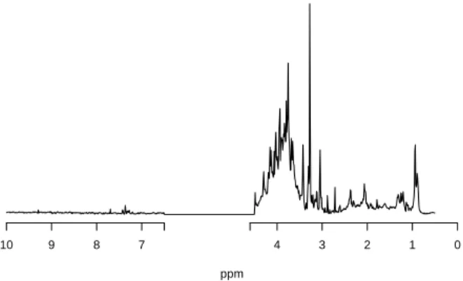
where Xiis a metabolomic profile (hence a curve, as shown in Figure 1), HRi
80
is the daily dose ingested by the corresponding mouse (HRi ∈ {0, 3, 9} and
81
di is the number of days from the beginning of the experiment up to the
82
spectrum acquisition (di ∈ {1, . . . , 21}). More precise information about the
83
data can be found in [Domange et al., 2010]. 84
The issue of interest is to predict the total dose of HR ingested, which is 85
the daily HR dose multiplied by the number of days of ingestion, from the 86
metabolomic data. This problem can be written as a regression problem: 87
yi = Φ(Xi) + ǫi (1)
where yi = HRi× di, Φ is the regression function to be estimated and ǫi is an
88
error term. This problem is motivated by several questions that frequently 89
arise in such an experimental settings: 90
• the first motivation is to know if the metabolomic profile alone is enough 91
to predict the drug dose ingested by an animal, which can be useful to 92
prevent an illness; 93
• conversely, the second motivation is to understand if the influence of 94
the HR dose ingestion is strong enough not to be seen as an artifact: if 95
yi can be accurately estimated from Xi then this is a strong indication
96
that the HR dose and more precisely, its cumulative effect, is really 97
disrupting the mouse metabolomic profile; 98
• finally the last motivation is to use the estimated regression function 99
to corroborate a set of relevant metabolites influenced by the HR in-100
gestion. The chosen approach is to extract the explanatory variables 101
(i.e., the part of the metabolomic profiles) with the strongest predictive 102
power, from the estimated regression function. 103
2.2
Data pre-processing
104
The data, acquired with 1
H NMR technique, are transformed as described 105
in [Domange et al., 2008] to obtain 397 spectra consisting in an intensity 106
distribution with 751 (non zero) variables. This step can be seen as a routine 107
designed to transform the original continuous signal into a discrete one, thus 108
to ease its analysis. An example of a resulting spectrum is given in Figure 1. 109
[Figure 1 about here.] 110
In order to recover the continuity of the signal, discrete wavelet decom-111
position is performed on the pre-processed spectrum: this is one of the most 112
commonly used signal transformation approach and it is particularly well 113
suited for uneven and chaotic signals, such as metabolomic profiles. Addi-114
tionally, the normal growth of the mice influences the metabolomic profile. 115
As this effect could be mixed with the total HR dose ingested by the mice 116
(which also depends on the day of measurement), a correction, based on 117
the control group’s quantiles alignment, is also performed on the wavelet 118
coefficients. This correction is based on the assumption that, other the con-119
trol group, no distribution variation in the metabolomic profiles should be 120
seen: the group’s quantile alignment is a robust method leading to compa-121
rable metabolomic profiles distributions each day, in the control group. This 122
method is quite standard in such cases (see, e.g., what is done for microarray 123
normalization in the R package limma, for instance [Bolstad et al., 2003]). 124
In the remaining, the obtained wavelet coefficients are denoted by 125
(Wi)i=1,...,397 ⊂ RD where D is the number of wavelet coefficients used in
126
the regression method (it depends on the wavelet basis and also on the DWT 127
approach as described in Section 3.3 but in any case D < 751). 128
3
Methodological proposal
129
3.1
State-of-the-art on using DWT in regression
prob-130
lems
131
Wavelet transforms are often applied to signals as a pre-processing step be-132
fore the statistical analysis [Davis et al., 2007, Xia et al., 2007]. A threshold-133
ing approach on the discrete wavelet transform is then generally performed 134
in order to remove the smallest (and most irrelevant) detailed coefficients 135
from the spectra representation. Standard thresholding strategies are the 136
so-called “hard thresholding” that simply removes the smallest coefficients 137
and leaves the others unchanged and the “soft thresholding” that removes 138
the coefficients smaller than a given threshold and reduces the others from 139
the value of this threshold. Of course, the choice of the threshold is very 140
important and several solutions have been proposed: for instance, the SURE 141
and Universal policies are calculated from an estimation of the level of noise 142
and justified by asymptotic properties (see [Donoho and Johnstone, 1994, 143
Donoho, 1995, Donoho and Johnstone, 1995, Donoho et al., 1995]). Also, 144
[Nason, 1996] suggests to use a cross-validation criterion to choose the thresh-145
old and [Johnstone and Silverman, 1997] to rely on a different threshold for 146
each level. More recently, [Gonz`alez et al., 2013] shows that keeping solely 147
the finest details coefficients at the lowest decomposition level produces a 148
representation of the data having the ability to correct a putative baseline 149
default. 150
A natural approach to predict a phenotype from metabolomic profiles 151
expressed in the wavelet domain would then be to perform a threshold-152
ing prior to the application of a well chosen regression method (see, e.g., 153
[Xia et al., 2007]). But this methodology does not link the wavelet coef-154
ficients selection to the prediction purpose. An alternative solution is to 155
perform a variable selection method, that takes into account the target vari-156
able, before learning the regression or the classification function. In this 157
direction, [Alexandrov et al., 2009] uses a multiple testing approach with 158
a Benjamini & Hochberg adjustment to select the relevant wavelet coef-159
ficients in relation to a target factor variable before building a classifica-160
tion model (based on SVM) to predict it. [Saito et al., 2002] proposes to 161
select the wavelet coefficients that maximize the Kullback-Leibler diver-162
gence between estimated densities obtained for the various levels of a fac-163
tor target variable before learning a classification function on the basis of 164
the selected coefficients. Also, [Jouan-Rimbaud et al., 1997] uses a “Rele-165
vant Component Extraction” that thresholds the less informative wavelet 166
coefficients from a PLS between the spectra and a target variable of inter-167
est. These latter approaches explicitly focused on wavelet coefficients se-168
lection but any feature selection method is expendable for such a task (see 169
[Liu and Motoda, 1998, Guyon and Elisseeff, 2003] for reviews about feature 170
selection). Feature selection algorithms can be time consuming and it has 171
also been pointed out in [Raudys, 2006] that they can lead to feature over-172
selection that hinders the prediction performances. 173
Another approach is to simultaneously select the variables and opti-174
mize the prediction error: [Alsberg et al., 1998b] select the wavelet co-175
efficients that minimize the cross validation error of a PLS regression. 176
Model selection methods penalize the prediction error with a quantity de-177
pending on the number of variables involved in the regression (see, i.e., 178
[Biau et al., 2005, Rossi and Villa, 2006] for examples in a similar framework 179
where the signal is projected onto an orthogonal basis for classification pur-180
pose where the data are functions). However, model selection requires the 181
definition of a relevant penalty term that can be hard to choose effectively, 182
as pointed out in [Fromont and Tuleau, 2006]. 183
3.2
A sparse one-phase approach
184
More recently, sparse methods [Tibshirani, 1996] have been intensively de-185
veloped because they allow the selection of the relevant predictors during 186
the learning process in an efficient and elegant way. The prediction error is 187
penalized by the L1
norm of the parameters of a linear model and it can be 188
proved that this leads to nullify some of the parameters in an optimal way. 189
Our proposal is to use penalized regression methods to simultaneously 190
define a regression function and select the most important wavelet coefficients 191
involved in the definition of this regression function. More precisely, the 192
numerical variable of interest (here, the total HR dose ingested by the mice, 193
(yi)i) is predicted from the metabolomic spectra through a penalized linear
194
model where the predictors are all the wavelet coefficients (without prior 195
thresholding). More precisely, the regression function Φ in Equation 1 is 196
estimated by a penalized linear regression on the wavelet coefficients (used 197
instead of Xi as predictor variables): ˆφ(Wi) = WiTβˆwhere
198 ˆ β = arg min β∈RD 1 397 X i kyi− WiTβk 2 RD+ λp(β) where kzk2 RD = PD j=1z 2 j. 199
Depending on the form of the penalization, p(.), the method is likely to 200
perform a rough or less rough variable selection: 201
• if p(β) = kβkL1 = PD
j=1|βj|, the linear regression is a sparse linear
202
regression also named LASSO [Tibshirani, 1996]. It selects wavelet 203
coefficients, in the set of D original coefficients, in a optimal way for 204
prediction purpose; 205
• if p(β) = kβk2RD, the linear regression is a ridge regression which tends 206
to produce β with small norms but does not perform a selection of the 207
wavelet coefficients; 208
• if p(β) = (1 − α)kβk2RD + αkβkL1, α ∈]0, 1[ the linear regression is 209
the so-called “elasticnet” method [Zou and Hastie, 2005], proposed in 210
an attempt to use the advantages of the two previous penalties. As 211
LASSO, it selects a reduced number of wavelet coefficients involved in 212
the regression function but this number is usually larger than the one 213
obtained when using the LASSO method. 214
Using a sparse linear regression method, such as LASSO or elasticnet, 215
then leads to perform a thresholding that is adapted to the regression task. 216
Moreover, the thresholding is made in a joint way, leading to select a common 217
set of wavelet coefficients for all the spectra (contrary to standard threshold-218
ing that nullify a different set of wavelet coefficients for each spectrum). This 219
property is likely to help prevent overfitting. Finally, sparse regressions lead 220
to the selection of a very limited number of coefficients that can, eventually, 221
help the interpretation (see Section 4 for a discussion and a comparison of the 222
different numbers of selected wavelet coefficients according to both methods). 223
3.3
Comparison methodology
224
The comparisons aim at understanding how the different approaches per-225
forms in predicting the total dose of HR ingested by mice. Different wavelet 226
approximations and regression methods are combined. More precisely, 227
• the possible wavelet approximations applied to the pre-processed data 228
(as described in Section 2.2) are raw spectra (no wavelet approxima-229
tion), wavelet coefficients (Haar or D4 bases), thresholded wavelet co-230
efficients (D4), undecimated wavelet detailed coefficients (D4). 231
“thresholded wavelet coefficients” correspond to the wavelet coefficients 232
that remain positive after a soft threshold with SURE policy and “un-233
decimated wavelet detailed coefficients” correspond to the union of the 234
finest details coefficients of the original spectra with the finest de-235
tails coefficients of the shifted spectra (obtained using the approach 236
of [Beylkin, 1992, Gonz`alez et al., 2013]). When using the full wavelet 237
decomposition or the “undecimated wavelet” approach, the dimension-238
ality of the original problem, D = 751 is left unchanged whereas the 239
“thresholded wavelet” approach leads to a dimensionality reduction 240
(D = 71 for D4 DWT), which is a standard way to handle large dimen-241
sion regression tasks. 242
• the possible regression method applied to the wavelet coefficients are 243
sparse or regularized regression methods as described in Section 3.2 244
(LASSO, ridge regression and elasticnet), PLS regression, which is a 245
standard approach when dealing with a large number of variables and 246
random forest [Breiman, 2001], as a basis for a comparison with non-247
linear methods. 248
For a sake of simplicity, only the following combinations are compared: 249
• any wavelet approximation is combined with the elasticnet regression. 250
Our proposal is to use the full wavelet decomposition (without thresh-251
olding) with a sparse regression method. To enlighten the uselessness of 252
the thresholding when using a sparse regression method, thresholding 253
is also combined with elasticnet in the comparison; 254
• the full wavelet decomposition is also combined with any regression 255
method described above. 256
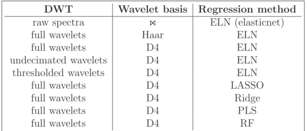
A total of 9 combinations are thus compared, summarized in Table 1. 257
[Table 1 about here.] 258
In order to train and to evaluate each of these combinations, the following 259
methodology is applied: 260
Wavelet transform First, the data are or are not preprocessed by a DWT. 261
The obtained coefficients are also scaled (each coefficient is centered to 262
a zero mean and scaled to a standard deviation equal to 1). 263
Split The observations (i.e., the pairs (Wi, yi)i) are randomly split into a
264
training set ST and a test set SV with balanced sizes (approximatively
265
200 observations each) taking into account the proportion of observa-266
tions in the groups defined by sex, dose (including the control group 267
to train the regression function so that it can predict when the animal 268
is not affected by HR ingestion) and day of measure. To estimate the 269
methods variability, this step is repeated 250 times giving 250 training 270
sets and the corresponding test sets. 271
Train The regression method is then applied to each training set. Several 272
methods involve hyper-parameters that have to be tuned: for random 273
forest, the hyper-parameters are the number of trees, the number of 274
variables selected for a given split, ... They are set to the default val-275
ues, coming from useful heuristics; the stabilization of the out-of-bag 276
error is achieved using that strategy. 277
For sparse and regularized linear regressions, an optimal λ is auto-278
matically selected through a regularization path algorithm (see, e.g., 279
[Efron et al., 2004] for the LARS algorithm in the case of LASSO). 280
Additionally, for elasticnet, the mixing coefficient α is set to 0.5 which 281
was the best choice according to other experiments in which α was 282
varied in {0.1, 0.25, 0.5, 0.75} (not shown in this paper for a sake of 283
simplicity). 284
Finally, for PLS, the number of kept components (between 1 and 40) is 285
tuned by a 10-fold cross-validation strategy performed on the training 286
set. 287
Test The root mean square error (RMSE) is calculated for each approach 288
involved in the comparison and for all the corresponding test sets: 289 RM SEV = s 1 nV X i∈SV (yi− ˆyi) 2
where nV is the number of observations in the test set and ˆyi is the
290
estimation of the total dose of HR ingested. 291
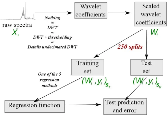
The methodology described above is illustrated in Figure 2. It leads to 292
obtain nine sets of 250 test errors, one for each combination of a wavelet 293
transform and regression algorithm. 294
[Figure 2 about here.] 295
All the simulations are performed using R free software 296
[R Development Core Team, 2012] and the packages wavethresh 297
[Nason and Silverman, 1994] (for wavelet facilities), glmnet 298
[Zou and Hastie, 2005] (for sparse and regularized linear methods), mixOmics 299
[Lˆe Cao et al., 2009] (for PLS) and randomForest [Liaw and Wiener, 2002] 300
(for random forest). 301
4
Results and discussion
302
This section presents the results of the experiments described in Section 3. 303
Section 4.1 is devoted to the comparison of the numerical performances of 304
the various combinations. The differences between the approaches (including 305
the number of wavelet coefficients selected) are discussed. Then, Section 4.2 306
extracts relevant features from the best combination of wavelet preprocessed 307
and regression method and compares it with a previously known list. This 308
provides another point of view on the relevance of the combination of the 309
DWT with sparse and regularized linear models for metabolomic data anal-310
ysis, this time as a feature selection method. The biomarkers that are the 311
most involved in the prediction of the total dose of HR ingested are selected 312
using an importance measure. The overall methodology is general enough to 313
be expandable for any regression method. 314
4.1
Numerical performances comparison
315
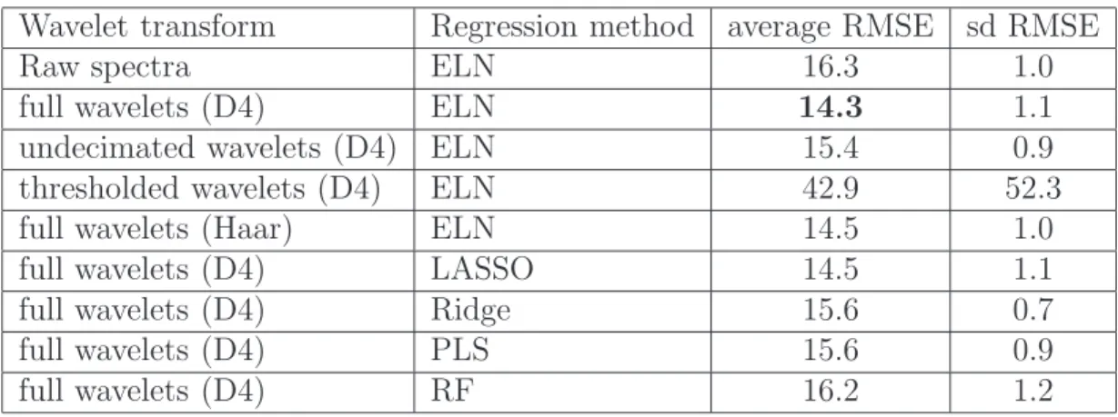
The averaged RMSE over the 250 test sets as well as their standard deviations 316
are reported in Table 2. 317
[Table 2 about here.] 318
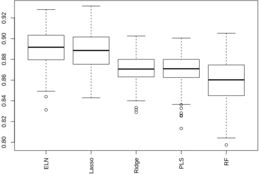
In addition, the boxplot of the R2
over the 250 test sets1
are given in 319
Figure 3 for the case where the data are expanded on the D4 basis and 320
where all wavelet coefficients are kept. 321
[Figure 3 about here.] 322
For the best method (combination of a DWT on a D4 basis with elasticnet), 323
the mean R2
is equal to 89.00% which is quite satisfactory. Thus, the ac-324
curacy of the prediction on the sample test is good enough to be used as 325
a relevant method to estimate the total dose of HR ingested by the animal 326
from the metabolomic profile alone. 327
Conversely, being able to predict the HR ingestion from the metabolomic 328
profile is a proof that the disrupting effect of HR on the metabolism is not an 329
artefact because an accurate relation between both variables is established. 330
Contrary to a test approach, that would have lead to test each part of the 331
metabolomic profile, this approach enlighten the strength of the relation 332
between the whole metabolomic spectrum and the target variable, here the 333
HR dose. Moreover, it does not even require the use of a control group. 334 1R2= 1 − P n Test i=1 (yi− ˆyi)2 PnTest i=1 (yi− ¯y)2 where ¯y= 1 nTest PnTest i=1 yi.
4.1.1 Comparison of the wavelet transforms 335
The first conclusion arising from Table 2 is that the wavelet transform effect 336
is stronger than the choice of the regression method. In particular, using the 337
wavelet coefficients remaining after a soft thresholding results in less accurate 338
predictions than using all the wavelet coefficients or even than the direct use 339
of the raw data. 340
Moreover, using all the wavelet coefficients in combination with a sparse 341
approach (elasticnet or LASSO) is the most accurate method; the impact 342
of the basis choice (D4 or Haar) is almost negligible. Undecimated wavelet 343
transform is the second most accurate wavelet transform approach: this may 344
be the indication that the coefficients with the finest details contain most 345
of the useful information for the prediction task. Maybe, an optimal trade-346
off would be to select wavelet coefficients at several scales, leaving only the 347
coefficients at the crudest scales. 348
To assess the significance of these conclusions, paired t-test were com-349
puted to compare the RMSE of the various wavelet transforms: the differ-350
ences between the use of Haar or D4 wavelets are not significant (at level 351
1%) but the differences between the use of all D4 wavelet coefficients and the 352
use of either the raw spectra, the D4 undecimated wavelet approach or the 353
D4 thresholded coefficients are all significant. Note that, even if the differ-354
ences between the averaged RMSE seem to be small, they are calculated over 355
250 replica which is a large enough number to provide confidence in these 356
conclusions. 357
4.1.2 Comparison of the regression methods 358
Comparing the regression methods, those that are (at least partially) based 359
on a sparse regularization, such as elasticnet and LASSO, obtain the best 360
results. Ridge regression is not as accurate as the methods based on a sparse 361
regularization but its variability is lower. Actually, combining a ridge and a 362
sparse penalty in the elasticnet seems to slightly decrease the variability of 363
the elasticnet results compared to those of the LASSO (except for two outlier 364
samples). Moreover, the influence of the mixing parameter α is not really 365
strong: test errors for elasticnet with α = 0.1, 0.25 or 0.75 are not shown in 366
the paper but would have mostly lead to the same conclusion: α = 0.1 or 367
0.25 has slightly deteriorated (but comparable) test errors, whereas α = 0.75 368
has test errors closer to the LASSO. 369
Finally, PLS, that is probably better suited for explanatory purpose, does 370
not give very satisfactory predictive performances in this case study but also 371
has a low variability. Here, random forest is the method that gives the worst 372
accuracy and also the largest variability of the performances over the 250 373
test sets. 374
Once again, the significance of these conclusions can be assessed by paired 375
t-tests: the differences between RMSE obtained by elasticnet and RMSE 376
obtained by ridge regression are significant. Of course, the same remark holds 377
for the comparison between elasticnet and any method performing worse 378
than ridge regression. This leads to the conclusion that the combination of a 379
DWT and a sparse linear method, such as elasticnet, is indeed a good choice 380
to handle regression problems where the predictors are metabolomic data. 381
4.1.3 Number of selected wavelet coefficients 382
Section 3.2 explains that using a sparse method on all the wavelet coefficients 383
can be seen as a joint thresholding adapted to the target variable. Then, it is 384
interesting to compare the numbers of coefficients selected by sparse methods 385
to the number of coefficients selected by a classical thresholding approach. 386
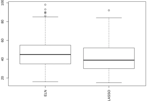
For D4 basis, 71 wavelet coefficients remain after the soft thresholding phase. 387
The numbers of selected coefficients over the 250 regression functions pro-388
vided by elasticnet and lasso are given in igure 4. 389
[Figure 4 about here.] 390
The average number of selected coefficients is often much smaller than the 391
one obtained with the classical thresholding approach. For instance, the best 392
method (elasticnet) selects 46.5 wavelet coefficients on average. Hence, not 393
only are the “one-phase” approaches faster and more accurate, they also 394
select less (but more relevant, according to the increase in accuracy) wavelet 395
coefficients. 396
4.2
Important biomarkers extraction
397
The relevance of the application of elasticnet on all the wavelets coefficients 398
is assessed by using the learned regression function, obtained in the previous 399
section, in order to extract the most important features related to the total 400
dose of HR ingested. A natural approach would be to directly analyze the 401
variables selected by the sparse regression but, because of the wavelet trans-402
form preprocessing, these are not directly linked to the spectra locations that 403
are of interest. 404
Alternatively, a standard approach, for linear models, is to select the 405
most important variables by the p-values of the coefficients associated to 406
the variables; this approach is not reliable in our context, both because it 407
only selects the most important wavelet coefficients (and, once again, not the 408
spectra locations) and also because if the explanatory variables are highly 409
correlated, the results of such tests are strongly related to the variables that 410
are used in the model. A small change in the list of explanatory variables 411
can lead to a very different list of significant variables and thus, the approach 412
is not really reliable in the case of a large number of explanatory variables. 413
To overcome these difficulties and to achieve the study of the influence 414
of the original variables (and not of the wavelet coefficients) in the predic-415
tion, we used a generalization of the importance measure originally designed 416
for random forest [Breiman, 2001]. This approach provides a way to assess 417
the relevance of biomarkers, to quantify their respective implications in the 418
biological phenomenon and thus to corroborate a list of biomarkers already 419
extracted elsewhere. In the following, Section 4.2.1 describes our approach 420
whereas Section 4.2.2 analyzes the results. 421
4.2.1 A measure of the importance of the variables 422
L. Breiman proposes the calculus of an “importance” measure to assess the 423
relevance of each explanatory variable in a random forest [Breiman, 2001]. 424
This measure is based on the observations that are not used to train a given 425
tree (out-of-bag observations): the values of the explanatory variable under 426
study are randomly permuted and the importance is defined as the decrease 427
of the accuracy (in terms of increased mean square error for a regression 428
problem) between the predictions made with the real values and those made 429
with the randomly permuted values. The more the MSE increases, the more 430
important the variable is for prediction. This approach was proven to be suc-431
cessful in variable selection in [Archer and Kimes, 2008, Genuer et al., 2010]. 432
We propose to use a similar approach to describe the way a wrong value for 433
a given variable (here a given value in the spectrum) propagates through the 434
wavelet transform and the regression function and affects the accuracy of the 435
final prediction of the total dose of HR ingested ingested by the mouse. This 436
analysis is focused on the best regression approach, i.e., the use of all wavelet 437
coefficients coming from a D4 basis expansion combined with elasticnet. As in 438
the approach proposed in [Breiman, 2001], the importance is calculated from 439
observations that are not used during the training process. More precisely, 440
the 250 test samples described in Section 3.3 are used to calculate importance 441
measures: the “importance” of a variable is the mean rate (over the test 442
sets) of MSE increase after a random permutation of its values among the 443
individuals (the other variables remaining with their true values). The idea 444
is to assess the prediction power of a variable by means of the prediction 445
accuracy disruption when this variable is given false values. The process is 446
repeated for the 751 variables corresponding to spectra locations, as described 447
in Algorithm 1. It can handle the way a given part of the spectra affects the Algorithm 1 Variables importance calculation
1: for each explanatory variable, v of the data set do {Variable loop}
2: Randomization Randomize the values of v for the 397 observations. The new explanatory variables (spectra) with randomized values for v are denoted by (Xv
i)i;
3: Wavelet expansion Calculate the wavelet coefficients with a D4 ex-pansion for (Xv
i)i. These are denoted by (Wiv)i; 4: for each test set, SV do {Test set loop}
5: Mean square error calculation Calculate the MSE based on the explanatory variables (Wv
i )i∈SV, MSEv,SV;
6: Importance calculation for SV Compare MSEv,SV to the original MSE obtained for the test set SV, MSESV: Iv,SV = 1 −
MSESV MSEv,SV;
7: end for
8: Importance calculation for variable v Average over the T = 250 test samples: Iv = P Test setsIv,SV T . 9: end for 448
quality of the prediction of the total dose of HR ingested. It thus gives an 449
assessment to the most relevant features in metabolomic spectra (i.e., the 450
features that contribute the most to an accurate prediction of the HR dose), 451
despite the series of transformations done. 452
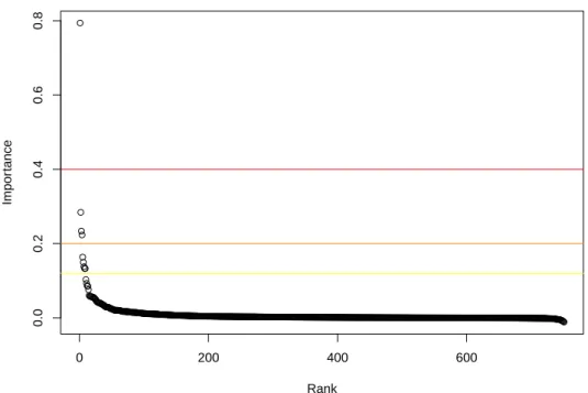
4.2.2 Results of the biomarkers extraction and comments 453
Figure 5 gives the importance of the 751 original variables (spectra locations) 454
ranked by decreasing value. 455
[Figure 5 about here.] 456
One variable is clearly much more important than all the other ones because 457
random permutations of its values cause an increase of almost 80% in MSE. 458
Three other variables seem to be important (with importance greater than 459
20%) and another group of 5 variables are also important to a lesser extent 460
(between the yellow line and the orange line in Figure 5). 461
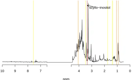
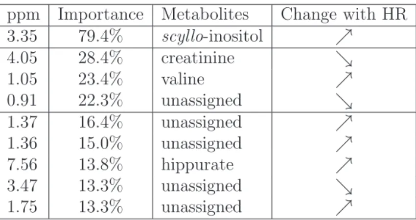
The list of the “most important” spectra locations and the names of the 462
associated metabolites (when it is known) are given in Table 3. Moreover, 463
the location of these metabolites in a1
H NMR spectrum is shown in Figure 6. 464
[Table 3 about here.] 465
[Figure 6 about here.] 466
The most important metabolite is the scyllo-inositol which was also identified 467
as an important metabolite in [Domange et al., 2008]. The other metabolites 468
emphasized by the variable importance (creatinine, hippurate, valine) were 469
also present in the original work: this confirms the reliability of our proposal. 470
Other spectra locations, that do not correspond to known metabolites, are 471
also identified by the variable importance. Noticing the relevance of the 472
most important metabolites found by our approach, these unknown peaks are 473
indications for further biological analysis to find new metabolites involved in 474
the poisoning process. 475
Also, some differences arise when comparing this list with the list 476
of biomarkers identified in [Domange et al., 2008]. Part of these dif-477
ferences may be explained by the fact that the dependent variable in 478
[Domange et al., 2008] is the daily HR dose ingested (i.e., a factor variable 479
with 3 levels) whereas, here, the total ingested dose was used in order to take 480
into account the cumulative effect of the ingestion. But it is also the positive 481
counterpart of not using a test approach and thus avoiding the standard false 482
positive issue that comes with them. As the extracted spectra locations are 483
directly related to the quality of the prediction, they are more reliable, even 484
if not so well theoretically justified. 485
Finally, not only does this approach give a list of important spectra lo-486
cations (corresponding to the total dose of HR ingested) but it also provides 487
a quantification of the influence of the spectra location on the accuracy of 488
the prediction. In our problem, scyllo-inositol therefore appears as the most 489
important metabolite affected by HR ingestion because its randomization 490
causes an 80% increase of the average MSE. 491
5
Conclusion
492
Wavelet transformation is commonly used to deal with spectrometric data in 493
biology, especially for de-noising purposes. Moreover, this paper shows that, 494
associated with a convenient learning method, it improves the understanding 495
of the relation between metabolomic spectrum and a phenomenon of interest 496
(for instance, metabolic disruptions linked to HR ingestion). It is also shown 497
that using a de-noising approach, not related to the variable to be predicted, 498
can lead to a dramatic loss of information. More precisely, some important 499
variables seem to be located in parts of the spectra that could be seen as 500
“minor” details. It is thus important to combine the wavelet transform and 501
de-noising with the purpose of the study. Sparse methods, that combine 502
a regression model and a variable selection seem to be well suited to this 503
task: they perform a kind of joint thresholding of the wavelet coefficients 504
that is directly related to the target variable. In particular, elasticnet gave 505
the best performance in prediction and was also able to provide a relevant 506
list of biomarkers, linked to the target variable, in our case study. 507
In conclusion, the combination of DWT with elasticnet can be used to ac-508
curately predict a numerical variable of interest from the metabolomic profile. 509
It is also useful to identify and confirm the most important features involved 510
in the biological process under study thanks to the importance measure in-511
troduced in this article. 512
6
Acknowledgements
513
The authors are grateful to Matthias De Lozzo and Cindy Hulin for providing 514
help support in programming during their Master project in INSA Toulouse. 515
References
516
[Alexandrov et al., 2009] Alexandrov, T., Decker, J., Mertens, B., Deelder, 517
A., Tollenaar, R., Maass, P., and Thiele, H. (2009). Biomarker discovery 518
in maldi-tof serum protein profiles using discrete wavelet transformation. 519
Bioinformatics, 25(5):643–649. 520
[Alsberg et al., 1998a] Alsberg, B., Kell, D., and Goodacre, R. (1998a). Vari-521
able selection in discriminant partial least-squares analysis. Analytical 522
Chemistry, 70:4126–4133. 523
[Alsberg et al., 1998b] Alsberg, B., Woodward, A., Winson, M., Rowland, 524
J., and Kell, D. (1998b). Variable selection in wavelet regression models. 525
Analytica Chimica Acta, 368:29–44. 526
[Archer and Kimes, 2008] Archer, K. and Kimes, R. (2008). Empirical char-527
acterization of random forest variable importance measures. Computa-528
tional Statistics and Data Analysis, 52:2249–2260. 529
[Beylkin, 1992] Beylkin, G. (1992). On the representation of operators in 530
bases of compactly supported wavelets. SIAM Journal on Numerical Anal-531
ysis, 29:1716–1740. 532
[Biau et al., 2005] Biau, G., Bunea, F., and Wegkamp, M. (2005). Functional 533
classification in Hilbert spaces. IEEE Transactions on Information Theory, 534
51:2163–2172. 535
[Bolstad et al., 2003] Bolstad, B., Irizarry, R., Astrand, M., and Speed, T. 536
(2003). A comparison of normalization methods for high density oligonu-537
cleotide array data based on variance and bias. Bioinformatics, 19(2):185– 538
193. 539
[Breiman, 2001] Breiman, L. (2001). Random forests. Machine Learning, 540
45(1):5–32. 541
[Cox and Cox, 2001] Cox, T. and Cox, M. (2001). Multidimensional Scaling. 542
Chapman and Hall. 543
[Davis et al., 2007] Davis, R., Charlton, A., Godward, J., Jones, S., Harri-544
son, M., and J.C., W. (2007). Adaptive binning: an improved binning 545
method for metabolomics data using the undecimated wavelet transform. 546
Chemometrics and Intelligent Laboratory Systems, 85:144–154. 547
[Domange et al., 2008] Domange, C., Canlet, C., Traor´e, A., Bi´elicki, 548
G. Keller, C., Paris, A., and Priymenko, N. (2008). Orthologous metabo-549
nomic qualification of a rodent model combined with magnetic resonance 550
imaging for an integrated evaluation of the toxicity of hypochoeris radi-551
cata. Chemical Research in Toxicology, 21(11):2082–2096. 552
[Domange et al., 2010] Domange, C., Casteignau, A., Pumarola, M., and 553
Priymenko, N. (2010). Longitudinal study of australian stringhalt cases in 554
France. Journal of Animal Physiology and Animal Nutrition, 94(6):712– 555
720. 556
[Donoho, 1995] Donoho, D. (1995). De-noising by soft-thresholding. IEEE 557
Transactions on Information Theory, 41(3):613–627. 558
[Donoho and Johnstone, 1994] Donoho, D. and Johnstone, I. (1994). Ideal 559
spatial adaptation by wavelet shrinkage. Biometrika, 81(3):425–455. 560
[Donoho and Johnstone, 1995] Donoho, D. and Johnstone, I. (1995). Adapt-561
ing to unknown smoothness via wavelet shrinkage. Journal of the American 562
Statistical Association, 90(432):1200–1224. 563
[Donoho et al., 1995] Donoho, D., Jonhstone, I., Kerkyacharian, G., and Pi-564
card, D. (1995). Wavelet shrinkage: asymptopia? Journal of the Royal 565
Statistical Society. Series B, 57(2):301–369. 566
[Efron et al., 2004] Efron, B., Hastie, T., Johnstone, I., and Tibshirani, R. 567
(2004). Least angle regression. The Annals of Statistics, 32:407–499. 568
[Fromont and Tuleau, 2006] Fromont, M. and Tuleau, C. (2006). Functional 569
classification with margin conditions. In Proceedings of the 19th Annual 570
Conference on Learning Theory, volume 4005 of Lecture Notes in Com-571
puter Science, pages 94–108. 572
[Genuer et al., 2010] Genuer, R., Poggi, J., and Tuleau-Malot, C. (2010). 573
Variable selection using random forests. Pattern Recognition Letters, 574
31:2225–2236. 575
[Gonz`alez et al., 2013] Gonz`alez, I., Eveillard, A., Canlet, A., Paris, T., 576
Pineau, P., Besse, P., Martin, P., and D´ejean, S. (2013). Undeci-577
mated wavelet transform to improve the classification of samples from 578
metabolomic data. JP Journal of Biostatistics. Forthcoming. 579
[Guyon and Elisseeff, 2003] Guyon, I. and Elisseeff, A. (2003). An intro-580
duction to variable and feature selection. Journal of Machine Learning 581
Research, 3:1157–1182. 582
[Johnstone and Silverman, 1997] Johnstone, I. and Silverman, B. (1997). 583
Wavelet threshold estimators for data with correlated noise. Journal of the 584
Royal Statistical Society. Series B. Statistical Methodology, 59:319–351. 585
[Jouan-Rimbaud et al., 1997] Jouan-Rimbaud, D., Walczak, B., Poppi, R., 586
de Noord, O., and Massart, D. (1997). Application of wavelet transform 587
to extract the relevant component from spectral data for multivariate cal-588
ibration. Analytical Chemistry, 69(21):4317–4323. 589
[Kim et al., 2008] Kim, S., Wang, Z., Oraintara, S., Temiyasathit, C., and 590
Wongsawat, Y. (2008). Feature selection and classification of high-591
resolution NMR spectra in the complex wavelet transform domain. Chemo-592
metrics and Intelligent Laboratory Systems, 90(2):161–168. 593
[Lˆe Cao et al., 2009] Lˆe Cao, K., Gonz´alez, I., and D´ejean, S. (2009). 594
*****Omics: an R package to unravel relationships between two omics 595
data sets. Bioinformatics, 25(21):2855–2856. 596
[Liaw and Wiener, 2002] Liaw, A. and Wiener, M. (2002). Classification and 597
regression by randomforest. R News, 2(3):18–22. 598
[Liu and Motoda, 1998] Liu, H. and Motoda, H. (1998). Feature Selection 599
for Knowledge Discovery and Data Mining, volume 454 of The Springer 600
Series in Ingineering and Computer Science. Springer, Nowell, MA, USA. 601
[Mallat, 1999] Mallat, S. (1999). A Wavelet Tour of Signal Processing. Aca-602
demic Press. 603
[Nason, 1996] Nason, G. (1996). Wavelet shrinkage using cross-validation. 604
Journal of the Royal Statistical Society. Series B. Statistical Methodology, 605
58:463–479. 606
[Nason and Silverman, 1994] Nason, G. and Silverman, B. (1994). The dis-607
crete wavelet transform in S. Journal of Computational and Graphical 608
Statistics, 3:163–191. 609
[R Development Core Team, 2012] R Development Core Team (2012). R: A 610
Language and Environment for Statistical Computing. Vienna, Austria. 611
ISBN 3-900051-07-0. 612
[Ramsay and Silverman, 1997] Ramsay, J. and Silverman, B. (1997). Func-613
tional Data Analysis. Springer Verlag, New York. 614
[Raudys, 2006] Raudys, S. (2006). Structural, Syntactic and Statistical 615
Pattern Recognition, volume 4109 of Lecture Notes in Computer Sci-616
ence, chapter Feature over-selection, pages 622–631. Springer-Verlag, 617
Berlin/Heidelberg, Germany. 618
[Rohart et al., 2012] Rohart, F., Paris, A., Laurent, B., Canlet, C., Molina, 619
J., Mercat, M., Tribout, T., Muller, N., Iannuccelli, N., Villa-Vialaneix, 620
N., Liaubet, L., Milan, D., and San Cristobal, M. (2012). Phenotypic 621
prediction based on metabolomic data on the growing pig from three main 622
European breeds. Journal of Animal Science, 90(12). 623
[Rossi and Villa, 2006] Rossi, F. and Villa, N. (2006). Support vector ma-624
chine for functional data classification. Neurocomputing, 69(7-9):730–742. 625
[Saito et al., 2002] Saito, N., Coifman, R., Geshwind, F., and Warner, F. 626
(2002). Discriminant feature extraction using empirical probability density 627
estimation and a local basis library. Pattern Recognition, 35:2841–2852. 628
[Tibshirani, 1996] Tibshirani, R. (1996). Regression shrinkage and selection 629
via the lasso. Journal of the Royal Statistical Society, series B, 58(1):267– 630
288. 631
[Wold, 1975] Wold, H. (1975). Soft modeling by latent variables; the non-632
linear iterative partial least square approach. J. Gani, Academic Press, 633
London. 634
[Wongravee et al., 2009] Wongravee, K., Heinrich, N., Holmboe, M., Schae-635
fer, M., Reed, R., Trevejo, J., and Brereton, R. (2009). Variable selection 636
using iterative reformulation of training set models for discrimination of 637
samples: application to gas chromatography/mass spectrometry of mouse 638
urinary metabolites. Analytical Chemistry, 81(13):5204–5217. 639
[Xia et al., 2007] Xia, J., Wu, X., and Yuan, X. (2007). Integration of 640
wavelet transform with PCA and ANN for metabolomics data-mining. 641
Metabolomics, 3(4):531–537. 642
[Zou and Hastie, 2005] Zou, H. and Hastie, T. (2005). Regularization and 643
variable selection via the elastic net. Journal of the Royal Statistical Soci-644
ety, series B, 67(2):301–320. 645
List of Figures
646
1 An example of metabolomic spectra from data discussed in 647
Section 2 (female mice of the control group at day 0). . . 36 648
2 Illustration of the methodology used to compare various com-649
binations of wavelet transforms and regression methods . . . . 37 650
3 Boxplots of the R2
of the mean square errors over the 250 test 651
sets for the prediction of the total dose of HR ingested with 652
various learning methods and a full representation with D4 653
wavelets. . . 38 654
4 Number of wavelet coefficients selected by elasticnet (ELN) 655
and LASSO over the 250 train sets for D4 wavelet expansion 656
using all the coefficients . . . 39 657
5 Importance of the 751 spectra locations ranked by decreasing 658
value. The horizontal lines separate increasing degrees of im-659
portance from above the red line (very important) to below 660
the yellow line (not important). . . 40 661
6 “Most important” metabolites locations on the1
H NMR spec-662
tra for the prediction of the total dose of HR ingested by the 663
mouse. The colors correspond to those of Figure 5. . . 41 664
ppm
10 9 8 7 4 3 2 1 0
Figure 1: An example of metabolomic spectra from data discussed in Sec-tion 2 (female mice of the control group at day 0).
Figure 2: Illustration of the methodology used to compare various combina-tions of wavelet transforms and regression methods
ELN Lasso Ridge PLS RF 0.80 0.82 0.84 0.86 0.88 0.90 0.92
Figure 3: Boxplots of the R2
of the mean square errors over the 250 test sets for the prediction of the total dose of HR ingested with various learning38
ELN LASSO 20 40 60 80 100
Figure 4: Number of wavelet coefficients selected by elasticnet (ELN) and LASSO over the 250 train sets for D4 wavelet expansion using all the coeffi-39
0 200 400 600 0.0 0.2 0.4 0.6 0.8 Rank Impor tance
Figure 5: Importance of the 751 spectra locations ranked by decreasing value. The horizontal lines separate increasing degrees of importance from above the40
ppm
10 9 8 7 4 3 2 1 0
scyllo−inositol
Figure 6: “Most important” metabolites locations on the 1
H NMR spectra for the prediction of the total dose of HR ingested by the mouse. The colors41
List of Tables
665
1 Approaches (wavelet transform and pre-processing combined 666
with a regression method) compared to predict the total HR 667
ingestion from the metabolomic profiles. . . 43 668
2 Means and standard deviations of root mean squared errors 669
for the prediction of the total dose of HR ingested with vari-670
ous combinations of wavelet transforms and regression meth-671
ods. “ELN” means “elasticnet”; “Ridge” means “ridge regres-672
sion”; “RF” means “random forest”; “D4” means “Daubechies 673
4 wavelet basis” and “Haar” means “Haar wavelet basis”. Bold 674
capitals are used to emphasize to the best method among all 675
experiments. . . 44 676
3 Summary of the “most important” peaks (and, if known, 677
metabolites) for the prediction of the total dose of HR ingested 678
by the mouse. . . 45 679
DWT Wavelet basis Regression method raw spectra ⋊⋉ ELN (elasticnet)
full wavelets Haar ELN
full wavelets D4 ELN
undecimated wavelets D4 ELN
thresholded wavelets D4 ELN
full wavelets D4 LASSO
full wavelets D4 Ridge
full wavelets D4 PLS
full wavelets D4 RF
Table 1: Approaches (wavelet transform and pre-processing combined with a regression method) compared to predict the total HR ingestion from the metabolomic profiles.
Wavelet transform Regression method average RMSE sd RMSE
Raw spectra ELN 16.3 1.0
full wavelets (D4) ELN 14.3 1.1
undecimated wavelets (D4) ELN 15.4 0.9 thresholded wavelets (D4) ELN 42.9 52.3
full wavelets (Haar) ELN 14.5 1.0
full wavelets (D4) LASSO 14.5 1.1
full wavelets (D4) Ridge 15.6 0.7
full wavelets (D4) PLS 15.6 0.9
full wavelets (D4) RF 16.2 1.2
Table 2: Means and standard deviations of root mean squared errors for the prediction of the total dose of HR ingested with various combinations of wavelet transforms and regression methods. “ELN” means “elasticnet”; “Ridge” means “ridge regression”; “RF” means “random forest”; “D4” means “Daubechies 4 wavelet basis” and “Haar” means “Haar wavelet basis”. Bold capitals are used to emphasize to the best method among all experiments.
ppm Importance Metabolites Change with HR 3.35 79.4% scyllo-inositol ր 4.05 28.4% creatinine ց 1.05 23.4% valine ր 0.91 22.3% unassigned ց 1.37 16.4% unassigned ր 1.36 15.0% unassigned ր 7.56 13.8% hippurate ր 3.47 13.3% unassigned ց 1.75 13.3% unassigned ր
Table 3: Summary of the “most important” peaks (and, if known, metabo-lites) for the prediction of the total dose of HR ingested by the mouse.