HAL Id: hal-03007152
https://hal.archives-ouvertes.fr/hal-03007152
Submitted on 9 Dec 2020
HAL is a multi-disciplinary open access
archive for the deposit and dissemination of
sci-entific research documents, whether they are
pub-lished or not. The documents may come from
L’archive ouverte pluridisciplinaire HAL, est
destinée au dépôt et à la diffusion de documents
scientifiques de niveau recherche, publiés ou non,
émanant des établissements d’enseignement et de
Prediction of the dynamics of a backward-facing step
flow using focused time-delay neural networks
Antonios Giannopoulos, Jean-Luc Aider
To cite this version:
Antonios Giannopoulos, Jean-Luc Aider. Prediction of the dynamics of a backward-facing step flow
using focused time-delay neural networks. International Journal of Heat and Fluid Flow, Elsevier,
2020, 82, pp.108533. �10.1016/j.ijheatfluidflow.2019.108533�. �hal-03007152�
Prediction of the dynamics of a backward-facing step
flow using Focused Time-Delay Neural Networks
Antonios Giannopoulosa,b,∗, Jean-Luc Aidera
a Laboratoire de Physique et M´ecanique des Milieux h´et´erog`enes (PMMH), UMR7636
CNRS, ESPCI Paris, PSL Research University, Sorbonne Universit´e, Univ. Paris Diderot, 10 rue Vauquelin, Paris, France .
bPhoton Lines Recherche, Parc Pereire Bat B, 99 rue Pereire, 78100 ,
Saint-Germain-en-Laye, France
Abstract
The full field dynamics of a separated, noise-amplifier flow, the Backward-Facing Step at Reh = 1385, have been identified by probe-like, upstream
measure-ments using an artificial Neural Network. Local visual sensors, coming from time-resolved Particle Image Velocimetry, were used as inputs and the dynamic Proper Orthogonal Decomposition coefficients were defined as goals-outputs for this non-linear mapping. The coefficients time-series were predicted and the instantaneous velocity fields were reconstructed with satisfying accuracy. The choices of inputs-sensors, training data-set size, hidden layer neurons and train-ing hyperparameters are discussed for this experimental fluid system.
Keywords: Backward-facing step flow, Neural Networks, Particle Image Velocimetry, Machine learning, System Identification
1. Introduction
Noise-amplifier flows are fluid systems which are globally stable, but which selectively amplify the upstream perturbations coming from random environ-ment noise by convective instability mechanisms [1, 2]. Typical examples are the flat plate Boundary Layer (BL) and Backward-Facing Step (BFS) flows [3, 4]. Noise-amplifier flows play an important role in many industrial flows, like separated flows around airfoils [5] and the complex 3D wakes of ground vehicles [6, 7]. Understanding and controlling these flows will be crucial for the drag minimisation and reduction of green-house gas emissions, which have to be de-creased in the European Union of at least 40 % by 2030, compared to the levels of 1990 [8]. A large portion of these emissions are due to ground vehicles, and a large portion of the ground vehicle emissions is due to aerodynamic drag [6, 9]. Controlling the shear layers to reduce the wake of a bluff-body or a ground
vehicle has been proved to be an efficient strategy to reduce the aerodynamic drag of ground vehicles [10, 11, 12, 13, 14].
In modern experimental and testing / measuring techniques, data-driven methods are becoming of great interest, since they don’t require a priori knowl-edge of a model and since the data-sets available are becoming larger and larger. This is especially true when studying thoroughly non-stationary flows for differ-ent Reynolds numbers with various sensors such as Particle Image Velocimetry (PIV) or multiple Pitot / multiple hot-wire probes. The increasingly powerful algorithms and computers let us handle and process quickly a large amount of data. Methods like statistical /regression and machine learning algorithms, su-pervised or unsusu-pervised, are becoming efficient and reliable for both academics or industrial applications. Neural networks particularly, are nowadays in the center of attention in this machine learning revolution we experience.
For complex flows, the number of degrees of freedom obtained from a 2D-2C (2-Components in a 2D velocity field) optical-flow Particle Image Velocimetry (PIV) measurement of a few millions pixels image is millions. Such a large system is impossible to control; a reduced-order model has to be identified. A dynamic observer can identify such a model based only on input-output mea-surements from measurable system quantities. As proposed firstly by [15] and verified experimentally for PIV data by [16, 17] it is possible to predict the full dynamics of a transitional flat-plate BL flow, in the form of Proper Orthogo-nal Decomposition (POD) coefficients, from local upstream measurements. The first step in their method was to create a successful reduced-order system using POD. The second step was to identify an optimal state-space model using a statistical learning process (the so-called N4SID algorithm), in order to predict at any moment all the POD coefficients (output) by measuring one or two local variables upstream (sensors or inputs) in the flow. A similar approach was also presented in a paper from Beneddine et al. [18], where the full frequency spec-trum was obtained from local frequency information of the flow. Time-resolved field reconstruction was also successfully obtained for time-resolved PIV data of a round jet flow using a point sensor and the mean field from [19].
In the present study, we explore means of performing this step of local-to-global dynamics system identification (SI) using a Neural Network (NN) archi-tecture. In this machine-learning data-driven identification process, we use a given data-set to learn the relation between local sensors and the global fluc-tuation dynamics of the system (in the form of POD coefficients) and a new data-set to validate the learning-training step. The identified NN coefficients will then allow the reconstruction of the full flow field, which would help design controllers targeting the kinetic energy of the full perturbation field. We will show the importance of the various choices (from sensors, to NN parameters) in a successful SI of an experimental time-resolved separated flow.
The paper is organised as follows. First, we present the various artificial NNs that can be found in the literature, and a brief review on their use in fluid mechanics problems. Then we present the experimental setup used to study the BFS flow. The choice of the NN architecture is then be discussed, together with the choice of the sensors characteristics and the training data size. The efficiency
of the chosen shallow NN architecture for such a SI is then demonstrated through the time-resolved velocity field reconstruction before turning to the conclusions.
2. Artificial Neural Networks
2.1. Definitions
Artificial Neural Networks (NN) are a subset of supervised Machine Learn-ing. They can provide a non-linear mapping between one set of inputs and a set of corresponding outputs. Great progresses have been made lately because of the availability of large data-sets, the increasing availability of multiple op-timised toolboxes and also the progress in Graphics Processing Units (GPU) parallel programming, which improves the computational speed. This is the reason why NNs are becoming more and more popular nowadays.
The fundamental part of a NN is the neuron or ”perceptron”. In general, one defines a weight wi associated to each ithneuron of the previous layer. To
obtain the output of a perceptron from a set on N neurons, one computes the sum of the N inputs multiplied by their corresponding weight and adds a given bias bi. An activation function f is then used to compute the output. A classic
activation function is a step-function, but more refined functions are usually needed. To improve the efficiency of classic NNs, it is possible to add one or many ”hidden layers” between the inputs and the outputs. Each hidden layer represents a non-linear function of linear combinations of its inputs, using a weight and a bias for each input. The inputs are then coming from the previous hidden layer. It is theoretically proven that any continuous function can be approximated with a single hidden layer [20, 21].
The simplest shallow, fully-connected NN architecture consists of the input layer (with n neurons), a single hidden layer (with an arbitrary number of n1
neurons) and a linear layer (with n2 = m neurons) connected to the output,
as shown in Fig. 1. A standard rule for the linear layer is to have the same number of neurons as the output layer. Regarding the choice of the number of neurons in the hidden layer, it can be as high as needed to increase accuracy, but without over-fitting. For a NN with a non-linear activation function f1 in the
hidden layer and a linear activation function f2in the linear layer, the equation
giving the kthneuron output of a single hidden layer network connected to the
jthneuron of the previous layer is:
yk= f1 n2 X j=0 w(2)kjf2( n1 X i=0 (wkj(1)xi+ bi) + bj (1)
where n1is the number of neurons in the first (hidden) non-linear layer and
. . .
Figure 1: An example of a shallow NN non-linear mapping to monitor m outputs Y using the n sensors X in a FTDNN architecture with k steps of delay and n1 neurons in the hidden
layer.
of the non-linear activation function f1, usually the popular tan-sigmoid or
hyperbolic tangent function is used:
f1(x) =
e2x− 1
e2x+ 1 (2)
The correct training process of the network (i.e. finding the optimal weights and biases connecting the neurons of different layers) consists of dividing the data-set into a training data-set and a validation data-set. Starting with the training data-set, the first set of weights connecting the layers is randomly ini-tialised for this first iteration. The error of the real vs the model-generated output is computed and the weights and biases are updated according to dif-ferent back-propagation schemes, in our case the Scaled Conjugate Gradient (SCG) method. In this case, the step size is adjusted at each iteration in order to minimise the performance function. The above process is called an ”epoch”. We continue the process for as many epochs as needed until a satisfactory fit error is achieved (Fig. 2). The second data-set, is the ”validation” data-set and is used to evaluate the performance of the network on new data and verify the achieved error, hence avoiding over-fitting.
2.2. Neural Network types
NNs can be divided into Feedback (or recurrent) and Feed-Forward. They can be discriminated according to their depth, either shallow or deep, depending on the number of hidden layers (one or more). Finally, they can also be divided into static or dynamic, if the output of the current step depends on the previous steps as well, giving it a notion of memory.
Figure 2: Block diagram of the NN System Identification training step.
In the case of a feed-forward NNs the output of any layer only modifies the next layer. System identification using feed-forward NNs have been a common practice since the 90s [22, 23]. Recently, deeper feed-forward NNs have also been implemented in complex SI cases [24].
The network used in the present SI study is a fully-connected Focused Time-Delay Neural Network (FTDNN) and is basically a standard feed-forward archi-tecture along with a tapped time-delay (of time-step size k) in the input. The term ”focused” comes from the fact that the notion of memory is introduced only in the input and not in the output. They were first introduced for speech recognition [25]. They are used to model long-range temporal dependencies by keeping a number of past measurements of the input at each k previous time steps xt−k leading to the following expression for the output of the system [26]:
yt= fw,b(xt, xt−1, ..., xt−k) (3)
where w and b are weight and bias parameters. On the other hand, in a recurrent NN, the system output is calculated from its previous past time-steps along with the input at the current time-step like in equation 4:
yt= fw,b(yt−1, xt) (4)
Recurrent NNs also introduce a notion of memory in the output of the sys-tem. One specific family of recurrent NN is the Non-linear Auto-Regressive eXogenous (NARX) models. They are autoregressive because the outputs of the current time step depends on the output of a number of previous steps. They are exogenous because the output depends also on a number of inputs. The NARX models were first introduced by [27] and used with NN with signifi-cant success by [28] for multiple non-linear SI cases. It is a natural extension of the Autoregressive Exogenous model (ARX), which has been extensively used
for supervised learning both in classification and prediction problems[29]. They were first developed by [30] to solve the vanishing or exploding gradient prob-lem of the back-propagated error. The difference with the FTDNNs, which also introduce an arbitrary long-term time dependence of the input to its pre-vious moments, is that the network is left to learn alone the size of the memory of each neuron during the training process. They do so using a sophisticated gate-neuron, that determines if the input is important enough or if it should be forgotten and when it should output its value. They are more computationally expensive to train than the FTDNNs.
2.3. Neural Networks in Fluid Mechanics
In fluid systems, feed-forward artificial NNs have been used for data-driven reduced-order modelling [31, 32, 33, 34, 35] with many results showing better field reconstruction than traditional POD methods [36, 37]. They were also used by [38] for experimental flow regime identification in multiphase flows. We mention that it has also been proved by [39], that a linear NN can be equivalent to a POD basis structure. Convolutional NNs have also been used for the efficient real-time 2D and 3D inviscid simulations [40] or along with pressure measurements for the velocity field prediction around a cylinder [41].
Furthermore, if there are hints or deeper understanding of the underlying physics, simple shallow NNs can provide very good results in SI [15, 42] as well as for control laws creation [43, 44, 45]. Their potential has been demon-strated early for modelling surface pressure and aerodynamic coefficients of 3-dimensional unsteady cases of aircrafts flows [46]. Finally, deep NNs are in-creasingly more important in the fluid mechanics community, especially for the modelling of complex turbulent flows. Srinivasan et al. [47] compared deep feed-forward and recurrent LSTM networks for turbulent shear flows predic-tion. Recently Deng et al. [48], used LSTM networks to reconstruct the POD coefficient time series using sub-sampled distributed velocity sensors in an in-verted flag flow PIV experiment. A short review of applications of deep NN to fluid mechanics can be found in [49].
3. Experimental setup
3.1. Hydrodynamic channel
Experiments have been carried out in a hydrodynamic channel in which the flow is driven by gravity, with a maximum free-stream velocity U∞ = 22 cm.s−1.
The flow is stabilised by divergent and convergent sections separated by hon-eycombs leading to a turbulence intensity of 0.8 %. A NACA 0020 profile is used to smoothly start the boundary layer. The test section is 80 cm long with a rectangular cross-section w = 15 cm wide and H = 10 cm high (Fig. 3). The step height is h = 1.5 cm. The maximum Reynolds numbers based on the step height is Reh,max = U∞h/ν ≈ 3000. The vertical expansion ratio is
h
w Shear Layer
H
Figure 3: Sketch of the BFS geometry and main flow features (shear layer and recirculation bubble). The PIV window is shown in grey and the visual sensor location shown as a red dot.
3.2. Lucas-Kanade Optical Flow PIV measurements
The flow is seeded with 20 µm neutrally buoyant polyamide particles, which are illuminated by a laser sheet created by a 2 W continuous laser (MX-6185, Coherent, USA) operating at 532 nm. A thin layer of fluorescent paint (FP Rhodamine 6G, Dantec) was applied to the illuminated surface to absorb the laser wavelength and avoid reflections and to allow correct near-wall measure-ments. The Camera used was a 4 Mp PCO DIMAX-cs with an acquisition frequency fac = 150 Hz. An narrow-band optical filter was mounted on the
camera to visualize only the laser light reflected by the particles. The length of the PIV window 11.2 h and its height is 3.7 h.
The time-resolved velocity fields are calculated from the acquisition of suc-cessive snapshots in the vertical symmetry plane at z = w /2, using a home-made Lucas-Kanade Optical Flow (LKOF) algorithm. The first version of the code has been developed at ONERA [50] and later modified, optimised and adapted to the constraints of real-time measurements by Gautier & Aider [51]. Among the advantages of the LKOF algorithm compared to a standard FFT-PIV algorithm is the calculation of a dense velocity field with one vector per pixel. It also allows for high computational speed when implemented on a GPU with CUDA functions [52]. The high spatial resolution is important for near-wall measurements while the high computation speed is important for real-time measurements that can be used as inputs in closed-loop flow control experi-ments [53]. The code has been used many times both for time-resolved PIV measurements with a high spatial resolution [54], as well as for closed-loop flow control experiments [51, 55]. The PIV calculations in the present study were performed on a NVIDIA TESLA K80 GPU.
4. Backward-Facing Step flow
4.1. Characterisation of the BFS flow
The objective of this study is to evaluate the potential of a NN SI method on experimental data of a shear-layer flow. We focus on a BFS flow which is a typ-ical case of noise-amplifiers. Upstream perturbations are amplified in the shear layer leading to significant downstream disturbances. Separation is imposed by a sharp edge creating a strong shear layer where Kelvin-Helmholtz instability leads to vortex shedding (Fig. 3). Another important feature is the creation of a large separation bubble, which is usually associated to pressure drag [56]. Its reduction is then a common objective to most flow control experiments targeting drag reduction. It is also considered as a benchmark case for the study of sep-arated flows. For this reason it has been extensively studied both numerically and experimentally [3, 57, 58]. The Reynolds number in the present experiment is Reh= 1385, corresponding to a free-stream velocity u∞ = 11 cm.s−1. The
incoming boundary layer, downstream from the leading edge, is laminar and follows a Blasius profile. The boundary layer thickness just upstream the step edge is δ0= 7mm = 0.5 h corresponding to a shape factor H = 2.3, typical of
a laminar boundary layer. The vortex shedding frequency is fshed = 1.13Hz,
which corresponds to a Strouhal number Sth=fshedU∞h = 0.15.
As we are interested in the growth and dynamics of coherent structures, one can also choose to monitor the vorticity field. Since vortical structures are embedded into the shear layer, it is better to use more refined criteria, like the Q criterium or the λCicriterium, which are well adapted to the identification of
vortical structures inside a shear layer. The λCicriterium was first introduced
by Chong et al. [59], who analysed the velocity gradient tensor D = −→∇−→u and proposed that the vortex core could be defined as a region where ∇u has complex conjugate eigenvalues. It was subsequently improved by Zhou et al. [60] and by Chakraborty et al. [61]. It was also successfully applied by [62], to visualise the 3D vortices created by a Jet in Cross-Flow measured by Volumetric Velocimetry, and by Gautier et al. [63] in a closed-loop flow control experiment using a similar visual sensor. For 2D data, λCi can be computed quickly and
efficiently using equation (5), when such a quantity is real (else λCi= 0):
λCi=
1 2
p
4 det(∇u) − tr(∇u)2 (5)
4.2. Proper Orthogonal Decomposition
Decomposing a dynamical system in modes of decreasing importance can help reducing the order of the variables of the system. N = 4197 consec-utive velocity fields {U (n) = (u∗x, u∗y)}n=1...N were computed from
consecu-tive flow snapshots ,with a sampling frequency of fac = 150 Hz. The size of
each snapshot-velocity field is 346 × 1010 pixels, with a spatial resolution of 0.166 mm/pixel . By calculating the mean field [Ux, Uy] we were able obtain
the velocity fluctuations u0x(t) = u∗x(t) − Ux and u0y(t) = u∗y(t) − Uy, which
1
3
5
7
9
11
x/h
3
2
1
y/h
5
10
10
-41
3
5
7
9
11
x/h
3
2
1
y/h
0
0.5
1
1
3
5
7
9
11
x/h
3
2
1
y/h
0
0.5
1
(b)
(x,y)=(0,0) x x x y(a)
y y Cisensor
velocity sensor
vortex
shedding
recirculation
<u
x>
t/u
u
x/u
Ci( s
-1)
(c)
Figure 4: Averaged streamwise velocity field (a), example of an instantaneous streamwise velocity field (b) and of an instantaneous swirling strength field (c) together with the position of the tested visual sensors. The flow is going from left to right. Movie online.
2 4 6 8 10 i 0 0.05 0.1 0.15 0.2 0.25 i ) 0.2 0.4 0.6 0.8 1 i )) i) Sum
Figure 5: Energy of each POD modes and cumulative total energy of the POD modes up to 80 % of the total energy.First two POD modes correspond to the vortex shedding due to the Kelvin-Helmholtz instability.
The fluctuation matrices organised in columns for each time-step were used to form the so-called ”snapshot matrix” to be decomposed. The reduced-order sys-tem is obtained using POD, which has been used extensively in fluid mechanics [64, 65]. It allows us to build a ranked and orthonormal basis containing N modes [66, 67]. The first K modes {Φk}k=1...K with K ≤ N containing a
suffi-cient percentage of the total energy is then chosen to compute the approximated velocity field ˜U (n): ˜ U (n) = K X k=1 hΦk, U (n)iΦk= K X k=1 ak(n)Φk (6)
where the scalar product h·, ·i is the energy-based inner product. The system output to be identified is obtained through the reduced state vector containing the K POD coefficients ak(n):
Y (n) = [a1(n) a2(n) ... aK(n)]T (7)
The full-field dynamics are now contained in their POD coefficients ak(t).
The balance between the order and accuracy of the POD reduced-order system is crucial, because it was seen that for a large number of POD modes the SI methods are much more likely to fail.
The energy of the individual POD modes as well as their cumulative energy are shown in Fig. 5. One can see that 50 % of the energy is contained in the three first modes. The system size containing at least 80 % of the total energy was used; that corresponding to K = 10 modes Φk and 10 POD coefficients
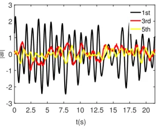
ak. The evolution of the 1st, 3rd and 5thPOD coefficients are shown in Fig. 6.
The characteristic frequency of the 1st POD mode corresponds to the Kelvin-Helmholtz frequency, i.e. the shedding of the vortices in the shear layer.
0 2.5 5 7.5 10 12.5 15 17.5 20 t(s) -3 -2 -1 0 1 2 3 |ai| 1st 3rd 5th
Figure 6: Time-series of 1st, 3rdand 5thdynamic POD coefficients.The evolution of the 1st
coefficient has a peak frequency close to the K-H vortex shedding frequency.
5. System Identification steps
In the present study we explore the potential of Artificial NNs for local-to-global dynamics SI applied to a shear layer flow. A full scheme of the identifica-tion process is summarised in Fig. 7. First, in the full data-set of time-resolved PIV experiment is decomposed to identify the dynamics in the form of POD coefficients. Then, in this data-driven identification process, we just rely on the input (sensors) - output offline measurements for a period of time from the operation of the plant. Once the machine (in our case an artificial NN) has mon-itored a sufficient number of realisations (training data-set), it will identify the relationship between the given input-sensor and the goal-output. If the method is successful, then monitoring the sensor will allow us to predict successfully the full global dynamics (in the form of POD coefficients) of the system in a new, unknown to the machine, data-set (validation), with no further need for a time consuming field decomposition analysis. Then the time-resolved field can be reconstructed from the identified NN-generated POD coefficients, using only the local sensor measurements.
In the following sections we discuss the influence of the main parameters on the SI process. We will especially show the importance of the choice of the physical parameters (nature, number and location of the sensors) in the ability of the SI learning process to find the proper NN weights and biases for each neuron. We will also show how the choice of the NN parameters (number of neurons in the hidden layer, time-delay) plays a crucial role in the efficiency of the SI process.
Figure 7: Sketch summarising the main steps of the identification procedure: from the time resolved PIV experiment to a convincing reconstruction of the velocity fields using local up-stream sensors.
6. Validation Criterion
To evaluate the efficiency of the identification, one has to define a quan-titative criterium to compare the POD coefficient time-series results obtained with the different NN architectures to the ones obtained experimentally. In the following, we compute the mean-squared error (MSE) at each time-step n for each POD coefficient ak(t):
M SEi= 1 N N X n=1 (aexp,i(n) − aN N,i(n)) 2 (8)
Then the averaged MSE for all the coefficients (m = 10) time-series gives the final evaluation error for the specific NN architecture:
M SE = 1 m m X k=1 ak (9)
7. Influence of the sensors definition
7.1. Choice of the sensor(s)
First, it is necessary to choose the physical quantities measured by the sen-sor(s). As the visual sensors are the inputs in the identification process, their choice is a critical step. The sensor(s) are necessarily based on the measurements
of the two components of the instantaneous 2D velocity fields at each time-step. Our challenge is to identify the birth and growth of vortical structures in the reciptivity process of the noise amplifier; in our case inside the shear layer right after separation. For this reason, possible sensors can be one or the two com-ponents of the fluctuation velocity field, the velocity magnitude or other vortex identification criteria, like the the λcicriterion.
7.2. Sensor position
The location of the sensor is critical. It should allow the detection of the perturbations during the initial phase of the reciptivity-amplification process of the shear layer [17, 15]. So in such a noise-amplifier flow the sensor was placed as upstream in the velocity field as possible, right after the separation in the high-shear region, as shown in Fig. 4. The proximity to the wall also is important for the method to be realistically applicable if other measuring devices, like hot-wires, were to be tested in the future. The exact sensor location was finally chosen to be kept slightly away from the wall (x = 0.25 h), in order to avoid possible noisy near-wall measurements. We mention that the flow field may be difficult to measure experimentally because of the large velocity gradients in the sensor region. Nonetheless, the good spatial resolution of the LKOF PIV measurements allows for the computation of gradient-based quantities like the vorticity or the swirling strength criterion.
7.3. Number and size of sensors
Reducing the number of sensors, as well as reducing the number of outputs, generally should make the training of the network simpler (lower order multiple input-multiple output regression). On the other hand, using less sensors may lead to a loss of valuable information about the flow, so a compromise has to be found. Single sensor configurations have been tested, i.e. either only vertical fluctuation velocity uy or λci, as well as combinations of two or three
sensors. The velocity component sensor s1is computed as an average in a five
neighbouring pixels window. The swirling strength vortex identification sensor s2 is defined as the sum of λCi computed over all the pixels in a dx = 15
pixels-wide window: s2= Z y2 y1 Z x2 x1 λCidxdy (10)
The height of the swirling strength window dyhas to be close to the thickness
of the shear, so that the vortex activity can be properly monitored. A good compromise has been obtained with dy = 0.5 h. The width of the swirling strength window also influences the quality of identification results. If it is too large, it creates an unnecessary smooth result, while if too small it can be too noisy, especially for gradient variables computed from experimental data. Finally, a window width of dx= 0.15 h was used.
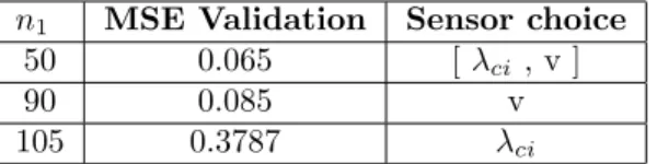
n1 MSE Validation Sensor choice
50 0.065 [ λci , v ]
90 0.085 v
105 0.3787 λci
Table 1: Comparison of the validation data-set fit error obtained with a single velocity sensor, a single swirling strength sensor and their combination. Using both sensors minimises the MSE and the number of neurons.
7.4. Choice of the sensor
The SI error obtained using the different sensors separately or combined can be found in Table 1. One can see that the choice of the sensor(s) is indeed critical. Using a single swirling strength sensor leads to a large MSE (37.87%) together with a large number of neurons (105). Using a single velocity sensor reduces the MSE (8.5%) but still needs a large number of neurons (90). Finally, the best results are obtained with the combination of the two sensors: the MSE is minimum (6.5%) and the number of neurons is strongly reduced (50).
This result can be explained. Indeed, both sensors being placed inside the shear layer just after separation, they contain a lot of information. This region is rich in frequencies coming from the the initial receptivity and amplification process together with the shear layer instability. This is also a region where measurement noise coming from the PIV measurement will be maximum. Using both sensors helps the identification from the NN to be successful in separating the physical from the unwanted frequencies, leading to a strong improvement of the MSE fit (6.5%).
8. Results and discussion
8.1. Optimal NN identification procedure
The goal of the NN identification method is to predict at each time step t the POD coefficients ak(t) of the full field using local upstream sensors sj(t).
The POD coefficients time-series have been calculated based on the PIV velocity fields. The sensors sj(t) were also monitored at the same time steps. The pairs
[ak(n), sj(n)] (n = 1 : 4197) is our identification data-set.
A FTDNN algorithm has been chosen. Our objective was then to identify the optimal sensors sj, the time delay k and the number of neurons in the hidden
layer n1. A basic scheme of the network is shown in Fig. 1. An anti-causal zero
phase low-pass moving average (over four time-steps) filter has been applied to each pixel time-series, to reduce slightly the measurement noise. We mention that the cut-off frequency of the filter is more than 10 times the vortex shedding frequency. For all the NN calculations (training and validation) the MATLAB Deep Learning Toolbox was used [68].
A NN should be as efficient as possible (according to the chosen criteria) and at the same time as simple as possible to easily check robustness and reduce computational time. Simplicity means minimising the number of layers and the
Network layer structure 2-50-10-10 Activation function Hyperbolic Tangent
Loss function MSE
Training method Scaled Conjugate Gradient
Time-delay (s) 2.66
Table 2: Final choice for the optimal NN architecture and its training hyperparameters.
Figure 8: Structure of the optimal FTDNN non-linear mapping, with 2 inputs-sensors (velocity and λCi), k = 400 steps of time-delay in the input, 1 hidden layer with n1= 50 neurons and
m = 10 POD coefficients as outputs.
number of neurons in each layer. The FTDNN networks tested used a tan-sigmoid transfer function and had a single hidden layer. In this case the NN is considered as ”shallow”.
The computational time for the training process, using a scaled conjugate gradient back-propagation algorithm, was of the order of O(1) minute using a Intel Xeon E5-2630 CPU running at 2.2 GHz. The low computational time allowed a full parametric test to find the optimal time delay k for the input and number of neurons n1for the hidden layer.
For each NN architecture, the full data-set [ak(t), sj(t)] (n = 1 : 4197) has
0 200 400 600 800
Epochs
0.1 1 10MSE
Training Validation50 100 150 200 250 300 350 400 k (time-steps) 0 0.2 0.4 0.6 0.8 1 MSE validation
NO IDENTIFICATION TRANSITIONAL IDENTIFIED
Figure 10: Evolution of the MSE as a function of the time-delay k in the sensor. Convergence is achieved for k higher than 300 time-steps.
been divided into training (85% of snapshots), validation (10% of snapshots) and over-fitting check data-set (5% of snapshots). The third data-set is used to monitor if high over-fitting is observed during training. In this case the process is stopped immediately. As a common practice, the data-set is shuffled randomly before the beginning of the training process. It avoids bad models if the data are initially classified. It also makes fitting faster because neighbouring points are not similar. Block consecutive data-set division failed to give good fit results. We also mention, that a data standardisation was applied before the training process to help handling different inputs or outputs with different scales. Lastly, the weights and biases of the network are initialised randomly for the first epoch. No early stopping criterion has been used.
The number of neurons of the hidden layer n1was always changed iteratively,
in order to find the optimal number leading to a minimization of the mean-squared error (MSE).
The same parametric study was carried out for the time-delay k, leading to a double loop parametric study from which the optimal combination of [k, n1]
was found. The optimal number of neurons for the hidden layer was found to be n1= 50 and the best sensor time-delay corresponded to k = 400 time steps
(2.66 s). A more detailed discussion about the time-delay parameter can be found below.
The results of the training performance as a function of the increasing epochs of the optimal architecture are shown in Fig. 9. 900 epochs were proved sufficient for a validation MSE error lower than 10 % for all POD coefficients. The optimal architecture and training parameters are summarised in the Table 2. This simple shallow FTDNN architecture (see Fig. 8) avoids the complexity of deeper architectures which increases the computational time for the training process and the need for a large amounts of training data [69], which are often difficult to obtain experimentally. This result verifies that shallow architectures
Figure 11: Network validation data-set performance as a function of the number of snapshots used for the training and the number of hidden layer neurons (n1) used.
Figure 12: Training and validation MSE for each POD coefficient time series.
can still provide satisfying results in many fluid mechanics applications [47, 37, 70].
8.2. Influence of the Time-Delay
The time-delay k in a FTDNN gives a notion of constant size memory in the sensors-inputs. It is crucial for the identification of downstream dynamics, while our sensors contain only information about the upstream dynamics (in the Kelvin-Helmholtz instability region). A sensitivity parametric study regarding the optimal time-delay in the inputs can be found by looking at the plot of the MSE of the validation data-set, as seen in Fig. 10. Keeping a time delay of k = 400 steps or 2.66 s, we can achieve a validation fit error less than 7%. k = 400 time-steps correspond in roughly 3 oscillations of the 1st mode ( which
This notion of ”memory” of these three events is crucial for the success of the algorithm. It explains why FTDNN with less memory or a standard feed-forward NN with zero time delay (k = 0) failed to identify the dynamics (M SE > 90%). An intermediate transitional region with k = 170 up to k = 300 might actually give good identification results, but it strongly depends on the random weight-bias initialisation and random shuffling of data. Convergence is achieved only for k > 300 time-steps.
8.3. Influence of the size of the training data-set
As expected for any data-driven method, the more informations are given to the machine the better. It will figure out more easily the optimal weights and biases for the mapping we ask it to perform. In Fig. 11 we can see that decreasing the number of snapshots used for the training of the network leads to an increase of the number of neurons in the hidden layer for an equivalent validation error (keeping a constant time-delay of k = 400 time steps). Above a given number of snapshots, increasing the number of neurons does not help, it just introduces over-fitting hence increasing the validation error. The BFS flow PIV experiment for Reh= 1385 is dominated by the vortex shedding frequency
(more than 40% of energy in the first two POD modes). Comparing the number of events (or oscillations) with the accuracy of the identification shows that to obtain a MSE lower than 10% we need to record at least 20 events.
8.4. Reconstruction of the instantaneous velocity fields
In Fig. 12 we present the results obtained for the ten first POD coefficients with the optimal double sensor and optimal time-delay configuration. We can see that the MSE for each POD coefficient is equivalent for all the coefficients at both training and validation, which proves we avoided over-fitting. In Fig. 13, we also present the time-series of three POD coefficients calculated from the experiment compared with the time-series obtained in the training step (a) and in the validation step (b) using the optimal NN architecture. Both training and validation data are in very good agreement with the experimental data and training and validation fit errors are very similar.
Projecting the NN-predicted POD coefficients ai to the POD modes Φi
al-lows the reconstruction of the fluctuation velocity fields of all time steps of the validation data-set. It is then possible to compare the predicted velocity field with the real experimental fields. The instantaneous experimental velocity field is compared to the one reconstructed with the optimal double visual sensor information as shown in Fig. 14 and corresponding video. In general, all the main features from the vortex shedding are apparent with correct amplitudes throughout the velocity field. Some smaller structures in the shear layer have reduced amplitude, due to the 80% energy cut during the time-resolved field decomposition, as well as the NN identification process error itself.
17.5 20 22.5 25 -2 0 2 a1
NN
data
5 7.5 10 12.5 15 -2 0 2 a1NN
data
17.5 20 22.5 25 -2 0 2 a3 5 7.5 10 12.5 15 -2 0 2 a3 17.5 20 22.5 25 t(s) -2 0 2 4 a5 5 7.5 10 12.5 15 t(s) -2 0 2 a5(e)
(d)
(a)
Training
(b)
(c)
(f)
Validation
Figure 13: Comparison of the 1st ,3rd and 5th POD coefficient time-series obtained from
experimental data with the ones obtained with NN for training (a, c, e) and validation (b, d, f) data-sets.
Figure 14: Comparison between experimental instantaneous streamwise fluctuation velocity field (a) and NN-reconstructed fields (b) using the double visual sensor and optimal NN architecture with n1 = 70 neurons in the hidden layer and N = 2728 training snapshots.
Movie online.
9. Conclusions
A successful application of a NN System Identification method to a time-resolved PIV experiment of a typical noise-amplifier flow has been presented. We were able to predict with satisfying precision the global dynamics of the flow (in the form of POD coefficients), using only two upstream visual sensors coming from local velocity measurements. A shallow FTDNN architecture was sufficient to recover the overall dynamics of the flow. There was no need for sophisticated LSTM gates or more than one hidden layers, which would increase the training complexity and the computational time.
It demonstrates the feasibility to reduce the order of such fluid systems from O(106) (for typical LKOF PIV measurements) to only a handful of useful vari-ables, which is crucial for control purposes. The final NN architecture allows us to predict the dynamics of the flow using local, upstream visual probes, without the need for time-consuming full- field decomposition analysis or in-trusive measuring devices like hot-wires or Pitot tubes. It was demonstrated that the combination of the swirling strength and local velocity sensors lead to a satisfying training and validation fit in the predicted POD coefficient time-series, even though these sensors were located in a high-gradient and difficult to measure region of the flow (early in the receptivity-amplification process of the noise-amplifier). The accuracy of the method was also illustrated in the instan-taneous velocity field reconstruction. The NN training process was found to be
very fast on a standard desktop computer (O(1) minutes). The double sensor approach is simple and fast to calculate and is ideal for a model-free closed-loop control scheme, like in [55, 71], with the objective to reduce the turbulent kinetic energy of the flow.
We also mention that, in a future implementation, the Reh number could
also be integrated as an input, while the output could include POD coefficients from the different Reh numbers, making it even more useful for flow control
purposes [36]. Distributed sensors, upstream and/or downstream, could also help achieve this complicated task. A larger number of POD modes could be included for more precise representation of the initial experimental data-set as well. Finally, the same methods can be also applied to other noise-amplifier flows, like the transitional flat plate boundary layer flow under the Tolmien-Schlichting instability.
Acknowledgements
The authors would also like to thank M. Aris Kanellopoulos from Georgia Institute of Technology for his valuable comments and discussions.
References
[1] P. Huerre, P. Monkewitz, Local and global instabilities in spatially devel-oping flows, Annual Review of Fluid Mechanics 22 (1) (1990) 473–537. doi:10.1146/annurev.fl.22.010190.002353.
[2] J. M. Chomaz, Global instabilities in spatially developing flows: non-normality and nonlinearity, Annu. Rev. Fluid Mech. 37 (2005) 357–392.
[3] J.-F. Beaudoin, O. Cadot, J.-L. Aider, J. E. Wesfreid, Three-dimensional stationary flow over a backwards-facing step, Eur. J. Mech. 38 (2004) 147– 155.
[4] G. Dergham, D. Sipp, J. C. Robinet, Stochastic dynamics and model re-duction of amplifier flows: the backward facing step flow, J. Fluid Mech. 719 (2013) 406–430.
[5] A. Darabi, I. Wygnanski, Active management of naturally separated flow over a solid surface. part 2. the separation process, Journal of Fluid Me-chanics 510 (2004) 105–129.
[6] J.-L. Aider, L. Dubuc, G. Hulin, L. Elena, Experimental and numerical investigation of the flow around a simplified vehicle model, in: Proc. Third MIRA International Vehicle Aerodynamics Conference, Rugby, England, 2001.
[7] J. F. Beaudoin, O. Cadot, J. L. Aider, K. Gosse, P. Paranthoen, B. Hamelin, M. Tissier, D. Allano, I. Mutabazi, M. Gonzales, J. E. Wesfreid, Cavitation
[8] E. EU-Council, European council, european council of 23 and 24 october 2014 conclusions.
[9] M. Grandemange, D. Ricot, C. Vartanian, T. Ruiz, O. Cadot, Charac-terisation of the flow past real road vehicles with blunt afterbodies, In-ternational Journal of Aerodynamics 4 (1-2) (2014) 24–42, pMID: 57797. doi:10.1504/IJAD.2014.057797.
[10] J. L. Aider, J. F. Beaudoin, J. E. Wesfreid, Drag and lift reduction of a 3D bluff-body using active vortex generators, Exp.in Fluids (DOI 10.1007/s00348-009-0770-y) (2009) 491–501.
[11] J. L. Aider, P. Joseph, T. Ruiz, P. Gilotte, Y. Eulalie, C. Edouard, X. Amandolese, Active flow control using pulsed micro-jets on a full-scale production car, Int. J. of Flow Control 6 (1) (2014) 1–20.
[12] Y. Eulalie, E. Fournier, P. Gilotte, D. Holst, S. Johnson, C. Nayeri, T. Schutz, D. Wieser, Active flow control analysis at the rear of an suv, International Journal of Numerical Methods for Heat ‘&’ Fluid Flow 28 (2018) 00–00. doi:10.1108/HFF-06-2017-0230.
[13] R. Li, D. Barros, J. Bor´ee, O. Cadot, B. R. Noack, L. Cordier, Feedback control of bimodal wake dynamics, Experiments in Fluids 57 (10) (2016) 158. doi:10.1007/s00348-016-2245-2.
URL https://doi.org/10.1007/s00348-016-2245-2
[14] M. Grandemange, D. Ricot, C. Vartanian, T. Ruiz, O. Cadot, Characteriza-tion of the flow past real road vehicles with blunt afterbodies, InternaCharacteriza-tional Journal of Aerodynamics 24 (1/2) (2014) 24–42.
URL https://hal-ensta.archives-ouvertes.fr/hal-01164775 [15] I. n. J. Guzm´an, D. Sipp, P. J. Schmid, A dynamic observer to capture and
control perturbation energy in noise amplifiers, Journal of Fluid Mechanics 758 (2014) 728–753.
[16] E. Varon, J. Guzman, D. Sipp, P. Schmid, J.-L. Aider, Experimental ap-plication of a dynamic observer to capture and predict the dynamics of a flat-plate boundary layer, in: Proc. of the 15th European Turbulence Conference (ETC15), Delft, The Netherlands, 2015.
[17] E. Varon, Closed-loop control of separated flows using real-time piv, Ph.D. thesis, ESPCI PARIS (2017).
[18] S. Beneddine, D. Sipp, A. Arnault, J. Dandois, L. Lesshafft, Conditions for validity of mean flow stability analysis, J.Fluid Mech. 798 (2016) 485–504. doi:10.1017/jfm.2016.331.
[19] S. Beneddine, R. Yegavian, D. Sipp, B. Leclaire, Unsteady flow dynamics reconstruction from mean flow and point sensors: an experimental study, Journal of Fluid Mechanics 824 (2017) 174201. doi:10.1017/jfm.2017. 333.
[20] G. Cybenko, Approximation by superpositions of a sigmoidal function, Mathematics of Control, Signals and Systems 2 (4) (1989) 303–314.
[21] K.-I. Funahashi, On the approximate realization of continuous mappings by neural networks, Neural Networks 2 (3) (1989) 183–192. doi:10.1016/ 0893-6080(89)90003-8.
[22] K. S. Narendra, K. Parthasarathy, Identification and control of dynamical systems using neural networks, IEEE Transactions on Neural Networks 1 (1) (1990) 4–27. doi:10.1109/72.80202.
[23] S. Reynold Chu, R. Shoureshi, M. Tenorio, Neural networks for system identification, IEEE Control Systems Magazine 10 (3) (1990) 31–35.
[24] O. Olekan, G. Xuejun, J. Steve, N. Gans, Nonlinear systems identification using deep dynamic neural networks, CS.
[25] A. Waibel, T. Hanazawa, G. Hinton, K. Shikano, K. J. Lang, Phoneme recognition using time-delay neural networks, IEEE Transactions on Acous-tics, Speech, and Signal Processing 37 (3) (1989) 328–339. doi:10.1109/ 29.21701.
[26] N. Charaniya, S. Dudul, Focused time delay neural network model for rainfall prediction using indian ocean dipole index, 2012, pp. 851–855. doi: 10.1109/CICN.2012.116.
[27] I. J. Leontaritis, S. A. Billings, Input-output parametric models for non-linear systems part i: deterministic non-non-linear systems, International Jour-nal of Control 41 (2) (1985) 303–328. doi:10.1080/0020718508961129. [28] S. Chen, S. Billings, P. Grant, Non-linear system identification using neural
networks, Neural Networks 51 (6). doi:10.1080/00207179008934126. [29] P. Vlachas, W. Byeon, Z. Yi Wan, T. P. Sapsis, P. Koumoutsakos,
Data-driven forecasting of high-dimensional chaotic systems with long-short term memory networks, Proceedings of the Royal Society A: Mathematical, Physical and Engineering Science 474. doi:10.1098/rspa.2017.0844. [30] S. Hochreiter, J. Schmidhuber, Long short-term memory, Neural
Compu-tation (1997) 1735–1780.
[31] S. M¨uller, M. Milano, P. Koumoutsakos, Application of machine learn-ing algorithms to flow modellearn-ing and optimization, Annual Research Briefs (1999) 169–178.
[32] O. San, R. Maulik, Neural network closures for nonlinear model order re-duction, physics.flu-dyndoi:705.08532v1.
identi-[34] A. Mohan, D. V. Gaitonde, A deep learning based approcah to reduced order modeling for turbulent flow control using lstm neural networks.
[35] S. Pan, K. Duraisamy, Long-time predictive modeling of nonlinear dy-namical systems using neural networks, Complexity 2018 (2018) 1–26. doi:10.1155/2018/4801012.
[36] O. San, R. Maulik, M. Ahmed, An artificial neural network framework for reduced order modeling of transient flows, Communications in Nonlinear Science and Numerical Simulation 77. doi:10.1016/j.cnsns.2019.04. 025.
[37] N. B. Erichson, L. Mathelin, Z. Yao, S. L. Brunton, M. W. Mahoney, J. N. Kutz, Shallow learning for fluid flow reconstruction with limited sensors and limited data, arXiv.
[38] Y. Mi, M. Ishii, L. Tsoukalas, Vertical two-phase flow identification using advanced instrumentation and neural networks, Nuclear Engineering and Design 184 (1998) 409–420.
[39] P. Baldi, K. Hornik, Neural networks and principal component analysis: Learning from examples without local minima, Neural Networks 2 (1) (1989) 53 – 58. doi:https://doi.org/10.1016/0893-6080(89)90014-2. URL http://www.sciencedirect.com/science/article/pii/ 0893608089900142
[40] J. Tompson, K. Schlachter, P. Sprechmann, K. Perlin, Accelerating eulerian fluid simulation with convolutional networks, in: Proceedings of the 34th International Conference on Machine Learning, 2016.
[41] X. Jin, P. Cheng, W.-L. Chen, H. Li, Prediction model of velocity field around circular cylinder over various reynolds numbers by fusion convolu-tional neural networks based on pressure on the cylinder, Physics of Fluids 30 (4) (2018) 047105. doi:10.1063/1.5024595.
URL https://doi.org/10.1063/1.5024595
[42] S.-C. Huang, J. Kim, Control and system identification of a separated flow, Physics of Fluids 20.
[43] C. Lee, J. Kim, D. Babcock, R. Goodman, Application of neural networks to turbulence control for drag reduction, Phys. Fluids 9 (1997) 1740–1747. doi:1070-6631.
[44] T. Herbert, X. Fan, J. Haritonidis, Laminar flow control with neural net-works 242 (1996) 87–91.
[45] J.Rabault, M. Kuchta, A. Jensen, U. Reglade, N. Cerardi, Artificial neu-ral networks trained through deep reinforcement learning discover control strategies for active flow control, physics.flu-dyndoi:arXiv:1808.07664v5.
[46] W. E. Faller, S. J. Schreck, Neural networks: Applications and oppor-tunities in aeronautics, Prog. Aerospace Sci. 32 (1996) 433–456. doi: 0396-0421(95)00011-9.
[47] P. A. Srinivasan, L. Guastoni, H. Azizpour, P. Schlatter, R. Vinuesa, Pre-dictions of turbulent shear flows using deep neural networks, Phys. Rev. Fluids 4 (2019) 054603. doi:10.1103/PhysRevFluids.4.054603.
URL https://link.aps.org/doi/10.1103/PhysRevFluids.4.054603 [48] Z. Deng, Y. Chen, Y. Liu, K. C. Kim, Time-resolved turbulent velocity
field reconstruction using a long short-term memory (lstm)-based artificial intelligence framework, Physics of Fluids 31 (7) (2019) 075108. arXiv: https://doi.org/10.1063/1.5111558, doi:10.1063/1.5111558. URL https://doi.org/10.1063/1.5111558
[49] J. Nathan Kutz, Deep learning in fluid dynamics, Journal of Fluid Mechan-ics 814 (2017) 1–4. doi:10.1017/jfm.2016.803.
[50] F. Champagnat, A. Plyer, G. Le Besnerais, B. Leclaire, S. Davoust, Y. Le Saint, Fast and accurate PIV computation using highly parallel iterative correlation maximization, Experiments in Fluids 50 (2011) 1169–1182. doi: 10.1007/s00348-011-1054-x.
[51] N. Gautier, J.-L. Aider, Control of the separated flow downstream of a backward-facing step using visual feedback, Proceedings of the Royal Soci-ety A: Mathematical, Physical and Engineering Sciences 469 (2160) (2013) 20130404. doi:10.1098/rspa.2013.0404.
[52] C.Pan, X.Dong, X.Yang, W.Jinjun, W.Runjie, Evaluating the accuracy performance of lucas-kanade algorithm in the circumstance of piv applica-tion, Sci China-Phys Mech Astron 58. doi:10.1007/s11433-015-5719-y. [53] N. Gautier, J.-L. Aider, Real-time planar flow velocity measurements using an optical flow algorithm implemented on gpu, Journal of Visualization 18 (2) (2015) 277–286. doi:10.1007/s12650-014-0222-5.
[54] E. Varon, Y. Eulalie, S. Edwige, P. Gilotte, J.-L. Aider, Chaotic dynamics of large-scale structures in a turbulent wake, Phys. Rev. Fluids 2 (2017) 034604. doi:10.1103/PhysRevFluids.2.034604.
URL https://link.aps.org/doi/10.1103/PhysRevFluids.2.034604 [55] N. Gautier, J.-L. Aider, T. Duriez, B. Noack, M.Segond, M.Agel,
Closed-loop separation control using machine learning, J.Fluid.Mech 770 (2015) 442–457.
[56] J. A. Dahan, A. S. Morgans, S. Lardeau, Feedback control for form-drag reduction on a bluff body with a blunt trailing edge, Journal of Fluid
[57] L. Hung, M. Parviz, K. John, Direct numerical simulation of turbulent flow over a backward-facing step, J. Fluid Mech. 330 (1997) 349–374.
[58] B. F. Armaly, F. Durst, J. C. F. Pereira, S. B., Experimental and theoretical investigation of backward-facing step flow, J. Fluid Mech. 127 (1983) 473– 496.
[59] M. Chong, A. Perry, B. Cantwell, A general classification of 3-dimensional flow fields, Physics of Fluids 2 (1990) 765–777.
[60] J. Zhou, R. Adrian, S. Balachandar, T. Kendall, Mechanisms for generating coherent packets of hairpin vortices, J Fluid Mech 387 (1999) 535–396.
[61] P. Chakraborty, S. Balachandar, R. J. Adrian, On the relationships between local vortex identification schemes, Journal of Fluid Mechanics 535 (2005) 189–214. doi:10.1017/S0022112005004726.
[62] T. Cambonie, J.-L. Aider, Transition scenario of the round jet in crossflow topology at low velocity ratios, Physics of Fluids 26 (8) (2014) 084101. arXiv:https://doi.org/10.1063/1.4891850, doi:10.1063/1.4891850. URL https://doi.org/10.1063/1.4891850
[63] N. Gautier, J.-L. Aider, Frequency-lock reactive control of a separated flow enabled by visual sensors, Experiments in Fluids 56 (1) (2015) 16. doi: 10.1007/s00348-014-1869-3.
URL https://doi.org/10.1007/s00348-014-1869-3
[64] J. Bor´ee, J., Extended proper orthogonal decomposition: a tool to analyse correlated events in turbulent flows, Experiments in Fluids 35 (2) (2003) 188–192. doi:10.1007/s00348-003-0656-3.
[65] M. Mendez, M. Raiola, A. Masullo, S. Discetti, A. Ianiro, R. Theunis-sen, J.-M. Buchlin, Pod-based background removal for particle image velocimetry, Experimental Thermal and Fluid Science 80 (2017) 181 – 192. doi:https://doi.org/10.1016/j.expthermflusci.2016.08.021. URL http://www.sciencedirect.com/science/article/pii/ S0894177716302266
[66] J. L. Lumley, The structure of inhomogeneous turbulent flows, in: A. M. Yaglom, V. I. Tatarski (Eds.), Atmospheric turbulence and radio propaga-tion, Nauka, Moscow, 1967, pp. 166–178.
[67] L. Sirovich, Turbulence and the dynamics of coherent structures, Quarterly of Applied Mathematics 45 (1987) 561–571.
[68] M. H. Beale, M. T. Hagan, H. B. Demut, Deep learning toolbox user’s guide.
[69] A. Canziani, A. Paszke, E. Culurciello, An analysis of deep neural network models for practical applications.
[70] B. D. Tracey, K. Duraisamy, J. J. Alonso, A Machine Learning Strategy to Assist Turbulence Model Development, 2017. arXiv:https://arc.aiaa. org/doi/pdf/10.2514/6.2015-1287, doi:10.2514/6.2015-1287. URL https://arc.aiaa.org/doi/abs/10.2514/6.2015-1287
[71] R. Li, B. R. Noack, L. Cordier, J. Bor´ee, F. Harambat, Drag reduction of a car model by linear genetic programming control, Experiments in Fluids 58 (8) (2017) 103. doi:10.1007/s00348-017-2382-2.