HAL Id: hal-00297488
https://hal.archives-ouvertes.fr/hal-00297488
Submitted on 5 Feb 2008
HAL is a multi-disciplinary open access
archive for the deposit and dissemination of
sci-entific research documents, whether they are
pub-lished or not. The documents may come from
teaching and research institutions in France or
abroad, or from public or private research centers.
L’archive ouverte pluridisciplinaire HAL, est
destinée au dépôt et à la diffusion de documents
scientifiques de niveau recherche, publiés ou non,
émanant des établissements d’enseignement et de
recherche français ou étrangers, des laboratoires
publics ou privés.
Solar modulation during the Holocene
F. Steinhilber, J. A. Abreu, J. Beer
To cite this version:
F. Steinhilber, J. A. Abreu, J. Beer. Solar modulation during the Holocene. Astrophysics and Space
Sciences Transactions, Copernicus Publications, 2008, 4 (1), pp.1-6. �hal-00297488�
F. Steinhilber, J. A. Abreu, and J. Beer
Eawag, Aquatic Science, Surface Waters – Radioactive Tracers, ¨Uberlandstrasse 133, 8600 D¨ubendorf, Switzerland Received: 22 August 2007 – Revised: 22 November 2007 – Accepted: 22 November 2007 – Published: 5 February 2008
Abstract. We built a composite of three reconstructions of
the solar modulation function over the Holocene. The re-constructions until 1950 are based on data from cosmogenic radionuclides and the present time (1951–2004) on neutron monitor data.
Interpreting our composite as an index of solar activity, we were able to compare the current solar activity with the last 9 300 years. During this time span 25 periods with similar high activity than the current period were found. That corre-sponds to about 15% of the time which lead to the conclusion that currently the Sun is very but not exceptionally active.
Our composite has a large potential for studies dealing with solar activity like the understanding of the solar dynamo and the reconstruction of solar forcing.
1 Introduction
Direct continuous observations of the solar activity have been started in about 1610 with the invention of the telescope. About 200 years later the famous Schwabe cycle was discov-ered. Additionally a long-term trend could be seen in the sunspot record. Soon people noticed a similarity between this long-term trend and temperature records. In particular periods which are characterized by a lack of sunspots such as the Maunder minimum (1645–1715) seem to coincide with cold climate conditions. To study this correlation a large vari-ety of time series of solar parameters have been continuously recorded in more recent times.
Unfortunately those time series do not provide any infor-mation about long-term trends. Hence they can not answer the question whether the Maunder minimum was a very ex-ceptional state or if such periods have been quite frequent, nor if the current solar maximum is very special or quite
Correspondence to: F. Steinhilber
common. However this information is very important for improving the solar dynamo models and estimating the past solar forcing. For this answer accurate solar activity recon-structions going as far back in time as possible are needed. So far only cosmogenic radionuclides can provide this infor-mation on millennial time scales. Such reconstructions were made several times.
Solanki et al. (2004) reconstruct sunspots for the last 11 000 years based on the cosmogenic radionuclide14C from tree rings. Their main result is that the current solar activity is exceptionally high. Their study shows that the last period when the Sun was as active as today was 8 000 years ago and that in 10% of the time the Sun was similar active as today.
Vonmoos et al. (2006) compare the solar modulation func-tions 8 during the Holocene (period 340 − 9 300 BP) us-ing 10Be from the Greenland Ice core Project (GRIP) ice core with14C from tree rings. They find slightly different 8 values for the two radionuclides which points to different non-solar signals in these proxies. But nevertheless both 8 records show similar long-term trends. Unfortunately a com-parison of the Sun during the Holocene with the current time is impossible since their reconstruction does not reach to to-day.
Muscheler et al. (2007) use the radionuclides 10Be and 14C to reconstruct the solar modulation function 8 for the past 1 000 years and come to a somewhat different result than Solanki et al. (2004). Their conclusion is that compared to the last 1 000 years the recent solar activity is high but not exceptionally high.
In order to resolve the discrepancies between the differ-ent long-term trends in the reconstructions we constructed a composite of reconstructions of the solar modulation func-tion bridging the values of Vonmoos et al. (2006) (cosmo-genic radionuclide10Be) with the modern instrumental data (neutron monitor data).
2 F. Steinhilber et al.: Solar modulation during the Holocene
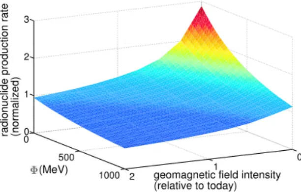
Fig. 1. Radionuclide production rate as a function of geomagnetic
field intensity and solar modulation function 8. In the calcula-tion, described in detail in Masarik and Beer (1999), protons and α-paticles are considered.
2 Theory: Solar modulation
The production of cosmogenic radionuclides depends on the intensity of cosmic ray particles (CRs) penetrating into the Earth’s atmosphere. Before CRs reach the Earth, they have to pass the heliosphere in which they are modulated.
The modulation of CRs is composed of different processes such as diffusion, adiabatic cooling, convection and drifts. These processes are included in the CR transport equation formulated by Parker (1965) which describes the propagation of CRs through the heliosphere and allows for calculating the CR spectrum everywhere within the heliosphere.
Gleeson and Axford (1968) found an approximation of that equation the so-called force-field approximation J (T , 8) = JLIS(T + 8)(T + 8)(T + 8 + 2TT (T + 2T0)
0)
(1) where JLIS is the local interstellar CR spectrum, T the ki-netic energy of the CRs and T0their rest energy. 8 describes the modification of the local interstellar spectrum (LIS) in the heliosphere. It has the unit of energy and is called solar modulation function.
As can be easily seen from Eq. (1) for 8 = 0 the modula-tion effect vanishes. The higher the solar modulamodula-tion the less CRs reach the Earth’s atmosphere and the less cosmogenic radionuclides (like10Be) are produced.
The usefulness of 8 to describe the CR spectra at 1 AU is shown by Caballero-Lopez and Moraal (2004). They compare experimental CR data with the spectrum obtained from Eq. (1) and with the spectrum calculated with the CR transport equation. They come to the conclusion that 8 is a good parameter to describe solar modulation at Earth (1 AU), if the considered CR particles have energies above 0.1 GeV/nucleon. This condition is fulfilled for the produc-tion of10Be as shown by McCracken (2004b).
Fig. 2. CR spectra calculated with Eq. (1) using the local
interstel-lar spectra of Webber and Higbie (2003), Castagnoli and Lal (1980) and Burger et al. (2000) for different values of the solar modula-tion funcmodula-tion 8 = 0 (dashed), 500 MeV (solid line) and 1 000 MeV (dotted). The cosmic ray energies T shown here are responsible for most of the10Be production (McCracken, 2004b).
3 Theory: Cosmogenic radionuclides 10Be and solar modulation
The radionuclide signal from ice cores is composed of three components: (1) solar activity (described by 8), (2) geomag-netic field intensity (mainly dipole moment component) and (3) system effects (geochemical behaviour).
Since we focus here on the solar activity the other two components have to be identified and removed.
The system component is the result of the transport of the radionuclides from the atmosphere to the terrestrial archive. They depend strongly on the geochemical properties of the considered radionuclide and the prevailing climatic condi-tions like the precipitation rate. McCracken (2004b) analyzes different averages of10Be data from Greenland and Antarc-tic and shows that the system effect component contributes less than 10% to the total signal when the data is averaged over 22 or more years.
The geomagnetic field acts as a shield for the charged CRs. Since its intensity varied significantly during the Holocene (shown in the top panel of Fig. 5) it has also a significant ef-fect on the radionuclide production and must be considered. This is done by using reconstructions of the geomagnetic field intensity. The magnetic field intensity is used to work out the so-called cutoff rigidity which says how much energy a CR needs to cross through the Earth’s magnetosphere.
To conclude the production rate of cosmogenic radionu-clides over the Holocene depends on the solar magnetic field described by the solar modulation function 8 and the geo-magnetic field intensity. As can be seen in Fig. 1 this de-pendence is non-linear. Here we used the calculations by Masarik and Beer (1999) based on Monte Carlo techniques.
FAA (O’Brien et al., 1996) NM/Deep River Castagnoli and Lal (1980) 1958 - 2007 monthly/annual 60 (6%)
4 Data
This work is based on three reconstructions of the solar mod-ulation function 8 summarized in Table 1. They were cho-sen because together they cover the period from today back to 9 300 BP.
In all reconstructions the influence of the geomagnetic field is considered. Vonmoos et al. (2006) use the reconstruc-tion of geomagnetic dipole component by Yang et al. (2000) and McCracken (2004b) make use of the geomagnetic field by McElhinny and McFadden (2000) who use in principle the same proxy data as Yang et al. (2000). Usoskin et al. (2005) use different cutoff rigidities depending on the loca-tion of the neutron monitor. Because the geomagnetic field has not changed significantly during their reconstruction pe-riod (1951 – 2004), the cutoff rigidities are kept constant.
The maximal standard deviation SD of the reconstruc-tion by McCracken et al. (2004a) is given to be 40 MeV. Usoskin et al. (2005) give values for the maximal SD which are 40 MeV after 1973 and 60 MeV for the period 1951 to 1973. The maximal SD of Vonmoos et al. (2006) is 80 MeV which takes into account the uncertainties of the10Be AMS (accelerator mass spectrometry) measurement and the geo-magnetic field intensity reconstruction.
Unfortunately the three reconstructions are based on dif-ferent local interstellar spectra (LIS) what leads to slightly different 8 values for the same radionuclide production rate. Hence we have to correct for the different LIS before we can build the composite.
5 Method of LIS-correction
To solve Eq. (1) the CR spectrum at 1 AU and the LIS have to be known. The CR spectrum can be worked out from cosmo-genic radionuclide production rate data (10Be concentrations, neutron monitor count rates), but the LIS, which describes the unmodulated CR spectrum outside the heliosphere, has to be estimated from CR intensity measurements inside the heliosphere. Different LIS are proposed to describe those
measurements. The LIS estimates differ depending on the energy as shown in Fig. 2.
Usoskin et al. (2005) give correction equations to convert 8 calculated with one LIS into 8 using another LIS. Their correction equations are obtained by comparing 8 derived from neutron monitor data. Here we used a more theoretical approach which is based only on Eq. (1) and artificial values of 8. Artificial means that we did not use experimental data but that we varied 8 in the interval of experimental data.
We did the following steps to obtain the LIS-correction equations:
1. Calculate the CR spectrum J0for a reference LIS = LIS0 with a fixed 80with Eq. (1)
2. Calculate the CR spectrum Jxfor a LISxwith a varying 8xwith Eq. (1) and find the CR spectrum Jx,fit which fits best the spectrum obtained with the reference LIS0 calculated in step 1.
3. Save 8x(Jx,fit) as a function of 80 4. Repeat steps 1 to 3 for different 80
5. Obtain the LIS-correction equation by applying a linear fit: 8x(Jx,fit) = m · 80(J0) + b
As reference LIS0 we chose the LIS by Castagnoli and Lal (1980). The index x in LISx and 8x means: x = C80 LIS by Castagnoli and Lal (1980), x = B00 LIS by Burger et al. (2000), x = W03 LIS by Webber and Higbie (2003). 80was varied from 0 to 1000 MeV. Corresponding to the response function of10Be given in McCracken (2004b), only protons with kinetic energies T between 0.5 GeV/nucleon and 5 GeV/nucleon were considered.
In Fig. 3 the solar modulation functions 8xusing the LIS by Burger et al. (2000) and Webber and Higbie (2003) are shown as a function of 80=8C80. It can be seen that the values of 8B00 are higher than the 8C80 values using the reference LIS. In contrast the values of 8W03 are shifted to smaller values.
4 F. Steinhilber et al.: Solar modulation during the Holocene
Fig. 3. Dependence of the solar modulation function 8x using
the LIS by Burger et al. (2000) and Webber and Higbie (2003) on 80=8C80 using the reference LIS by Castagnoli and Lal (1980). In a first order approximation the solar modulation functions 8 cal-culated using different LIS can be converted into each other by lin-ear functions.
As can be seen in a first order approximation the values of 8 using different LIS can be converted into each other by using linear functions which are called here LIS-correction equations. The LIS-correction equations to convert 8x to the reference 8C80 are:
8C80 = 1.04 · 8B00 − 73 MeV (2) 8C80 = 1.05 · 8W03 + 54 MeV (3) By combining these equations one can also find an equation to convert 8B00 into 8W03. Our correction equations com-pare well with Usoskin et al. (2005) (their Eqs. (A4)).
Our LIS-correction Eq. (2) was tested by comparing the reconstruction of Usoskin et al. (2005) with and without us-ing the LIS-correction with a reconstruction of 8 by FAA (US Federal Aviation Administration) also based on neutron monitor data but using our reference LIS. The calculations of the FAA are described in O’Brien et al. (1996) and the data can be found at http://www.faa.gov/education research/ research/med humanfacs/aeromedical/media/cari6exe.zip.
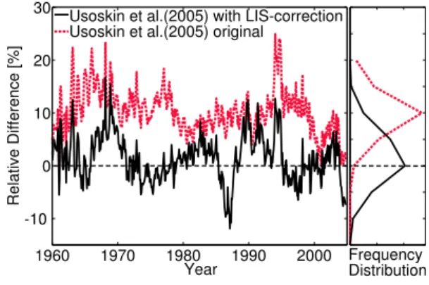
Figure 4 shows the relative differences between the data by FAA and by Usoskin et al. (2005) with and without the cor-rection. The frequency distribution confirms the correction leading to an average relative difference of zero.
The LIS-corrections from Eqs. (2) and (3) were used to correct the reconstructions of 8 in Table 1 for the differ-ent LIS. After all 8 values were corrected to the LIS by Castagnoli and Lal (1980) they were linearly interpolated to annual resolution to obtain a homogeneous time resolution for the whole reconstruction period. Finally a running-mean of 25 years was applied. The whole composite record which covers the past 9 300 years is shown in Fig. 5.
From the histogram in Fig. 6 we found the lowest value of the current solar activity to be 600 MeV. Defining that
Fig. 4. Relative difference of monthly averages of the solar
modula-tion funcmodula-tion 8 by US Federal Aviamodula-tion Administramodula-tion (FAA) and by Usoskin et al. (2005) without (original) and with LIS-correction using Eq. (2). left: in time; right: frequency distribution
Table 2. Periods with 8 values above the lowest value of the
25-year running mean during the period 1951-2004 (8 = 600 MeV), their durations and mean 8 values. Periods in bold lasted as long as the current period.
Period Period Duration Mean 8 no. (year BP) (years) (MeV)
1 8794 - 8745 49 695 2 8665 - 8638 27 624 3 8433 - 8412 21 619 4 5788 - 5760 28 616 5 5506 - 5492 14 617 6 5381 - 5362 19 617 7 5114 - 5101 13 607 8 4073 - 4018 55 699 9 3943 - 3914 29 625 10 3843 - 3816 27 614 11 3554 - 3533 21 613 12 2849 - 2811 38 663 13 2590 - 2534 56 678 14 2471 - 2387 84 712 15 2277 - 2249 28 623 16 2207 - 2143 64 692 17 1992 - 1940 52 647 18 1797 - 1744 53 668 19 1680 - 1599 81 790 20 1459 - 1427 32 628 21 1132 - 1100 32 622 22 1019 - 981 38 654 23 734 - 700 34 637 24 601 - 562 39 681 25 217 - 206 11 617 today (26) 25 - -54 80 650
value as lower limit of high solar activity we found 26 pe-riods of high solar activity in the composite. These pepe-riods are listed in Table 2. When using the given periods one must
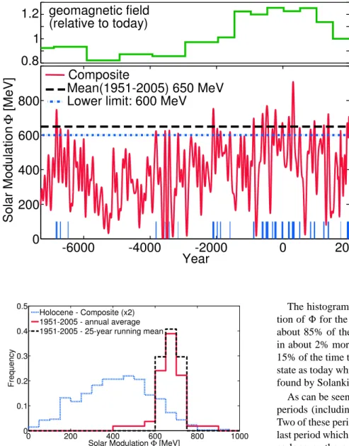
(red). The black dashed line shows the mean value of the 25-year run-ning mean (8 = 650 MeV) of the cur-rent Sun (1951–2004). The blue dot-ted dashed line is the lower limit (8 = 600 MeV) defining periods with high solar activity. The bars in the bot-tom show the periods with high solar activity (8 ≥ 600 MeV).
Fig. 6. Histogram of 8 values: during the Holocene 25-years
run-ning mean (blue) and for the current time 1951–2004, 1-year aver-ages (red) and 25-year averaver-ages (black). For better visualization the frequencies of the Holocene (blue) were multiplied by a factor of two.
be aware of the absolute uncertainties ( ≤ 50 years) of the ap-plied timescale (GRIP timescale ss09, Johnsen et al. (1997)). However the absolute uncertainties have only a minor influ-ence on the duration of the periods.
6 Discussion
Interpreting the solar modulation function as an index of so-lar activity allows for comparing the current soso-lar activity with the last 9 300 years.
The histogram in Fig. 6 compares the frequency distribu-tion of 8 for the whole composite with the last 50 years. In about 85% of the time the Sun was less, in 13% equal and in about 2% more active than today. Thus we found that in 15% of the time the Sun was in a similar or even more active state as today which is a higher percentage compared to 10% found by Solanki et al. (2004).
As can be seen from Table 2 during the last 9 300 years 26 periods (including today) occurred with high solar activity. Two of these periods lasted as long as the current period. The last period which showed similar high activity and also lasted as long as the current one was about 1 700 years ago. We found periods (No. 23–25 in Table 2) of high activity during the last 1 000 years which is in agreement with Muscheler et al. (2007).
7 Conclusions
Solar activity can be reconstructed using cosmogenic ra-dionuclides from terrestrial archives provided that geomag-netic intensity variability and climate effects are removed from the data.
McCracken et al. (2004a), Usoskin et al. (2005) and Von-moos et al. (2006) make use of cosmogenic radionuclides and reconstructed the solar modulation function for different periods. In this study a composite of these three data sets was built over most of the Holocene. Due to the fact that the three reconstructions are based on different local interstellar spec-tra, LIS-correction equations were derived which then were used to build the composite.
6 F. Steinhilber et al.: Solar modulation during the Holocene The LIS-correction equation between the LIS by Burger et
al. (2000) and Castagnoli and Lal (1980) was confirmed by a comparison of the reconstruction by Usoskin et al. (2005) with a reconstruction by the US Federal Aviation Adminis-tration.
The record provides the basis to study the solar activity in the past, to improve solar dynamo models and hopefully to develop a quantitative solar forcing function.
Acknowledgements. The authors would like to thank Horst
Ficht-ner for his helpful comments which improved this paper. This work was financially supported by NCCR Climate - Swiss Climate Research and by the ETH Zurich poly-project: Variability of the Sun and Global Climate.
Edited by: H.-J. Fahr
Reviewed by: H. Fichtner and another anonymous referee
References
Burger, R. A., Potgieter, M. S., and B. Heber: Rigidity de-pendence of cosmic ray proton latitudinal gradients mea-sured by the Ulysses spacecraft: Implications for the diffu-sion tensor, J. Geophys. Res., 105, A12, 27447–27456, doi: 10.1029/2000JA000153, 2000.
Caballero-Lopez, R. A. and Moraal, H.: Limitations of the force field equation to describe cosmic ray modulation, J. Geophys. Res., 109, A01101, doi:10.1029/2003JA010098, 2004.
Castagnoli, G. and Lal, D.: Solar Modulation Effects in Terrestrial Production of Carbon-14, Radiocarbon, 22, 133–158, 1980. Gleeson, L. J. and Axford, W. L.: Solar Modulation of Galactic
Cosmic Rays, Astrophys. J., 154, 1011–1026, 1968.
Johnsen, S. J., Claasen, H. B., Dansgaard, W., Gundestrup, N. S., Hammer, C. U., Andersen, U., Andersen, K. K., Hvidberg, C. S., Dahl-Jensen, D., Steffensen, J. P., Shoji, H., Sveinbj¨ornsd´ottir,
´
A. E., White, J., Jouzel, J., and Fisher, D.: The δ18O record along the Greenland Ice Core Project deep ice core and the problem of possible Eemian climatic instability, J. Geophys. Res., 102, 26 397–26 410, doi:10.1029/97JC00167, 1997.
Masarik, J., and Beer, J.: Simulation of particle fluxes and cosmo-genic nuclide production in the Earth’s atmosphere, J. Geophys. Res., 104, 12 099–12 111, 1999.
McCracken, K. G., McDonald, F. B., Beer, J., Raisbeck, G., and Yiou, F.: A phenomenological study of the long-term cosmic ray modulation, 850–1958 AD, J. Geophys. Res., 109, A12103, doi:10.1029/2004JA010685, 2004a.
McCracken, K. G.: Geomagnetic and atmospheric effects upon the cosmogenic10Be observed in polar ice, J. Geophys. Res., 109, A04101, doi:10.1029/2003JA010060, 2004b.
McElhinny, M. W. and McFadden, P. L.: Paleomagnetism: Conti-nents and Drifts, Academic, San Diego, California, 2000. Muscheler, R., Joos, F., Beer, J., M¨uller, S. A., Vonmoos, M.,
and Snowball, I.: Solar activity during the last 1 000 yr in-ferred from radionuclide records, Qua. Sci. Rev., 26, 82–97, doi:10.1016/j.quascirev.2006.07.012, 2007.
O’Brien, K., Friedberg, W., Sauer, H.H., and Smart, D.F.: Atmo-spheric cosmic rays and solar energetic particles at aircraft alti-tudes, Env. Inter., 22, 9–44, 1996.
Parker, E. N.: The passage of energetic charged particles through interplanetary space, Planet. Space Sci., 13, 9–49 ,1965. Solanki, S. K., Usoskin, I. G., Kromer, B., Sch¨ussler, M., and
Beer, J.: Unusual activity of the Sun during recent decades com-pared to the previous 11 000 years, Nature, 431, 1084–1087, doi:10.1038/nature02995, 2004.
Usoskin, I. G., Alanko-Huotari, K., Kovaltsov, G. A., and Mur-sula, K.: Heliospheric modulation of cosmic rays: Monthly re-construction for 1951–2004, J. Geophys. Res., 110, A12108, doi:10.1029/2005JA011250, 2005.
Vonmoos, M., Beer, J., and Muscheler, R.: Large variations in Holocene solar activity: Constraints from 10Be in the Green-land Ice Core Project ice core, J. Geophys. Res., 111, A10105, doi:10.1029/2005JA011500, 2006.
Webber, W. R., and Higbie, P. R.: Production of cosmogenic Be nu-clei in the Earth’s atmosphere by cosmic rays: Its dependence on solar modulation and the interstellar cosmic ray spectrum, J. Geophys. Res., 108, 1355–1365, doi:10.1029/2003JA009863, 2003.
Yang, S., Odah, H., and Shaw, J.: Variations in the geomagnetic dipole moment over the last 12 000 years, Geophys. J. Int., 140, 158–162, 2000.