Climate Change Vulnerability Assessment with Constrained Design of Experiments, Using a Model-Driven Engineering Approach

HAL Id: hal-02802688

https://hal.inrae.fr/hal-02802688

HAL is a multi-disciplinary open access archive for the deposit and dissemination of sci-entific research documents, whether they are pub-lished or not. The documents may come from teaching and research institutions in France or abroad, or from public or private research centers.

L’archive ouverte pluridisciplinaire HAL, est destinée au dépôt et à la diffusion de documents scientifiques de niveau recherche, publiés ou non, émanant des établissements d’enseignement et de recherche français ou étrangers, des laboratoires publics ou privés.

Climate Change Vulnerability Assessment with

Constrained Design of Experiments, Using a

Model-Driven Engineering Approach

Romain Lardy, Gianni Bellocchi, Bruno Bachelet, David Hill

To cite this version:

Romain Lardy, Gianni Bellocchi, Bruno Bachelet, David Hill. Climate Change Vulnerability Assess-ment with Constrained Design of ExperiAssess-ments, Using a Model-Driven Engineering Approach. 25th European Simulation and Modelling Conference (ESM), Oct 2011, Guimaraes, Portugal. pp.354-362. �hal-02802688�

CLIMATE CHANGE VULNERABILITY ASSESSMENT WITH

CONSTRAINED DESIGN OF EXPERIMENTS, USING A MODEL DRIVEN

ENGINEERING APPROACH

Romain Lardy(1,3,4), Gianni Bellocchi(1), Bruno Bachelet(2,3,4), David R.C. Hill(2,3,4) (1) Grassland Ecosystem Research Unit, French National Institute for Agricultural

Research (INRA), 234 Avenue du Brézet, 63100 Clermont-Ferrand, France (2) Clermont Université, BP 10448, F-63000 CLERMONT-FERRAND

(3) CNRS, UMR 6158, Université Blaise Pascal, LIMOS, F-63173 (4) ISIMA, Computer Science & Modelling Institute, BP 10125, F-63177

KEYWORDS

Climate Change Vulnerability, Experimental Design, Grassland Ecosystems, Model Driven Engineering

ABSTRACT

Vulnerability is the degree to which human and environmental systems are likely to experience harm due to a perturbation or stress. Vulnerability assessment under climate change needs a huge amount of simulations. The set of simulations needed depends on the uncertainties hypothesis. In this study, we propose an approach for vulnerability assessment with different types of design of experiments. We build up model of these designs, to identify a common pattern seen as metamodel, which models can be conformed to. In order to build up dedicated distribution platform for vulnerability analysis, we use a Model Driven Engineering approach.

INTRODUCTION

Vulnerability is the degree to which human and environmental systems are likely to experience harm due to a perturbation or stress (Kasperson et al. 2005). It has become in recent years a central focus of the global change (including climate change) and sustainability science research communities (Füssel 2007).

The purpose of vulnerability assessment is not only to determine which systems are the most vulnerable, but also to understand why they are so (Luers et al. 2003). This information is crucial in the process of determining strategies of adaptation to, or mitigation of the effects of change. In the context of climate change, this remains not enough studied (Easterling et al. 2007).

The literature contains many definitions of vulnerability, going from the notion of sensitivity (Dowing and Patwardhan 2005) to more complex ideas, yet tacking into account the exposure history of the system (Turner et al. 2003) up to residual impacts of climate change after adaptation (IPCC 2001). Due to the great number of sensitive parameters influencing climate change vulnerability, and because of the high level uncertainties in climate change impact studies (e.g. emission scenario, climate modelling, downscaling and initialization, and

modelling of the impacts on a target system), vulnerability assessment (which is partly correlated to sensitivity analysis) will necessary need many simulations. Moreover, taking into account potential adaptations means more assumptions and more simulations. It is clear that a pertinent Design of Experiment (DOE) will be absolutely necessary to reduce the time required for simulations. Such an amount of simulations also needs high performance computing, at least for the distribution of simulations. In this context, our paper presents an approach for climate change vulnerability assessment with constrained DOE, using a model driven engineering approach. This work is meant as a preliminary step towards software framework to deal with the distribution of experimental designs under vulnerability constraint.

In order to present our approach, we use ModVege (Jouven et al. 2006a), a mechanistic model for the dynamics of production, structure and digestibility of managed permanent pastures. This model has been retained to study the feasibility of our approach, because on the one hand, it is complex enough to reproduce climate variability impacts on a pasture (Jouven et al. 2006b) but on the other hand, it requires relatively few inputs and limited computational time. Our approach will then be applied to larger classical biogeochemical models typically used for this kind of studies (e.g. PaSiM, Graux et al. 2011).

This work is the continuity of the model-driven, reverse-engineering applied to design of experiment by Lardy et al. (2011). The remainder of the paper is structured as follows. The next section presents the ModVege model. The three following sections present the methodology used, with special focus on DOE and Model Driven Engineering (MDE). Then, we detail our vulnerability assessment methodology with a special spotlight on DOE and associated models. Our MDE approach is completed by the proposition of a metamodel of agro-ecological models with its associated DOE. This approach aims at proposing abstractions that will enable the distribution of experimental designs on high performance computing platforms.

MODEL DESCRIPTION

ModVege (Jouven et al. 2006a) is a multi-year, mechanistic model simulating the dynamics of production, structure and

digestibility of managed permanent pastures. It is designed to respond to various defoliation regimes, based on five assumptions. Firstly, the average value of the biological attributes of vegetation (functional traits) can explain the functioning of a permanent pasture (Louault et al. 2005). Secondly, sward heterogeneity can be modelled by the relative abundance of the structural plant components (Carrère et al. 2002) (i.e. green leaves and sheath, dead leaves and sheath, green stems and flowers, and dead stems and flowers). Thirdly, like many grassland dynamic models (e.g. HPM, Thornley 1998), senescence, growth and abscission can be modelled by continuous fluxes, calculated on daily-time step. Fourthly, due to reserves storage and mobilization in plant organs, shoot growth, based on a light-utilization efficiency approach, is modulated by a seasonal pattern (e.g. Volenec et al. 1996). The latter is considered as a functional trait. The last assumption is that the quality of green compartment, abscission and senescence are influenced by compartment ageing. The model was evaluated for upland grasslands in the Auvergne region of France (Jouven et al. 2006b).

DESIGN OF EXPERIMENTS

Design of experiments (DOE) has a rich history, with many theoretical developments and practical applications in a variety of fields. Since the beginning of computer simulation, DOE has been an active research field (Kempthorne 1952; Amblard et al. 2003). In the modelling field, DOE is a needed tool for efficiently testing and analysing the behaviour of a model (Kleijnen 1987). Most of model simulations aim at exploring and/or testing the behaviour of the model. A parameter or an input is called a factor in the DOE terminology, it could be either qualitative or quantitative (Kleijnen et al. 2005). Each factor can take two or more values, called levels of factors. An experimental design is a combination of factor levels.

Whatsoever for verification and validation or for the different models’ usage, a huge number of simulation runs

are necessary. In particular, for environmental dynamics modelling, models have become increasingly more complex at the pace of computer power. Due to the high number of parameters required by the model and to the computation time of a single run, the needed time for a full factorial DOE is usually too expensive for a sequential machine. This implies that, first of all we use smart but less complete DOE and, on top of that, we have to use distributed computing. The use of a proper DOE will help to get, firstly, all the information we are looking for. For example, in the case of sensitivity analysis, the DOE is important to get relevant sensitivity to all parameters without neglecting their interactions. The second point is to have the smallest number of simulations for the best quality results, thus implying optimization of the total computation time. Computation time is then considerably reduced thanks to the distribution of processes on parallel architectures.

SIMULATION WITH MODVEGE

The ModVege model, initially developed in Python, has recently been re-implemented in Java for the purpose of integration into a modelling platform. As most field-scale management decisions are taken on daily basis, the model runs on daily-time step.

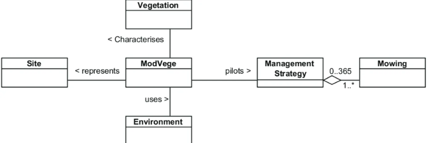
To sum up, model inputs can be grouped into four classes (Figure 1):

- Vegetation data, i.e. average functional traits of vegetation community (characteristics of functioning of the plant) and initial sward status (biomass and age of the four compartments), - Site properties, i.e. soil nutrition index and soil

water-holding capacity,

- Environment data (photosynthetically active radiation, air temperature, precipitations and potential evapotranspiration),

- The management strategy, which is composed of a number of mowing events.

Figure 1. UML metamodel of the ModVege input model

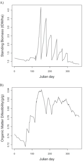
Few outputs generally are used, either for direct use or for coupling with other models (e.g. animal model). The most used are the standing and the digestibility of the grass. Figure 2 provides an example of result on upland grassland in the Auvergne region of France.

MODEL DRIVEN ENGINEERING

Model Driven Engineering (MDE) is part of software engineering that studies, since more than a decade, software development, maintenance and evolution with a unifying modelling approach (Favre et al. 2006). The Model Driven

Architecture (MDA) is a set of industry standard promoted by the Object Management Group (OMG). The separation between the descriptions of the platform independent system part (PIM, Platform Independent Model) and of the platform specific one (PSM Platform Specific Model) characterizes the MDA, whereas the MDE is a global integrative approach (Favre et al. 2006) for various technological spaces. MDE relies on three fundamental concepts: the “model”, the “metamodel” and the “transformation procedure”.

A)

B)

Figure 2. A) Standing biomass and B) digestibility of the grass on intensive permanent grassland at Marcenat, in the Auvergne region of France.

A model is a simplified representation of a system. The system is an entity modelled in order to study it, to understand it, and to predict in a mastered context other than reality. The model could be defined by the relation “is a representation of” between itself and the studied system (Hill 1996; Atkinson and Kuhne 2003; Seidewitz and Technologies, 2003; Bézivin 2004). Nevertheless, in the MDE context, this definition is not sufficient because it does not allow the model to become “productive” (i.e.

interpretable and exploitable by a machine). That is why many authors have preferred the following definition (Kleppe et al. 2003): “A model is a description of (part of) a system written in a well-defined language”, since it is more adapted to transformation procedures that enable models to become productive.

The notion of well-defined language indirectly points to the second MDE principle, i.e. the “metamodel”. Different definitions can be found in the literature: “a metamodel is a model that defines the language for expressing a model” (OMG 2002); “a metamodel is a specification model for a class of SUS (System Under Study) where each SUS in the class is itself a valid model expressed in a certain modelling language” (Kleppe et al. 2003). Unlike to the popular opinion, a metamodel is not a model of model, since it is better defined as a model of modelling language. This definition is based on the following relation: a model “is conform to” a metamodel. For instance, in the context of Object-Oriented Programming, if we consider the object as a model of reality, then the class is a metamodel and the object “is conform to” its class. However, metamodels can have specific forms depending on the technical domain such as:

Ͳ XML technologies: an XML file is conform to a Document Type Definition (DTD) or to an XML schema,

Ͳ language theory and compilation: a source code is conform to its grammar,

Ͳ in cartography, if our system is France, our model could be an IGN (French National Geographic Institute) map and its metamodel its legend: a map is conform to its legend,

Ͳ Standard Template Library (STL): a vector<int> is conform to Vector<T> metamodel.

MDE principles are relevant for all types of models, either object-oriented or not. MDE is not restrained to a technical domain.

Nevertheless, to get a productive model, it is necessary to describe how to transform it. This aspect corresponds to the third MDE concept: “transformation of model”. Unlike the two other notions, there is no consensus for its definition (Rahim and Mansoor 2008; Lano and Clark 2008; Iacob et al. 2008). According to Favre (2004), the relation could be defined as “is transformed in”. As for the metamodel, the transformation can take different forms under the technical domain (Favre et al. 2006), for example:

Ͳ eXtensible Stylesheet Language (XSLT) into XML language,

Ͳ compilation and code generation for language theory

Ͳ Model to Model: Atlas Transformation Language (ATL) 0 100 200 300 1 .0 1 .5 2 .0 2 .5 3 .0 3 .5 4 .0 Julian day S ta n d in g B io m a s s ( tD M /h a ) 0 100 200 300 0 .7 2 0 .7 4 0 .7 6 0 .7 8 0 .8 0 0 .8 2 0 .8 4 Julian day O rg a n ic M a tt e r D if e s ti b ili ty (g /g )

The Model Driven Engineering approach is in our case a good way to tackle the problem of designing a framework dealing with many types of experimental design and different ways to assess vulnerability.

VULNERABILITY ASSESSMENT METHODOLOGY A two-stage approach

Climate change vulnerability literature is rich on definitions. For example, Füssel and Klein (2006) identified three categories of vulnerability definitions:

- The “risk-hazard framework” definition. In this case, vulnerability is defined as response relation between an exogenous stress and its negative effects (Dowing and Patwardhan, 2003). This definition is rather similar to the sensitivity definition in the IPCC (2001).

- The social constructivist model. Here, vulnerability is seen as the set of socio-economic causes explaining the difference between sensitivity and exposure.

- The IPCC 2001 definition: “vulnerability is defined as the extent to which a natural or social system is susceptible to sustaining damage from climate change. Vulnerability is a function of the sensitivity of a system to changes in climate (the degree to which a system will respond to a given change in climate, including beneficial and harmful effects), adaptive capacity”. This definition is only centred on climate change, but could be easily extended: Vulnerability is the degree to which a human or environmental system is likely to experience harm before being damaged (Kasperon et al. 2003; Turner et al. 2003).

A few indicators exist in the literature on vulnerability assessment. In this publication, we will narrow their use to what is proposed by Luers et al. (2003) in their method. This vulnerability evaluation is based on four concepts: the state of the system relatively to a damage threshold, its sensitivity, its exposure history, and its adaptation capacity.

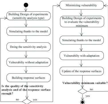
As we wish to evaluate different vulnerability assessments in a comparative fashion, depending on definitions, outputs of interest and tested hypotheses, we will need to be able to deal with vulnerability with or without adaptation. This is why we propose a two-step approach (Figure 3):

1. Firstly, a sensitivity analysis step, whose aim will be to estimate vulnerability without adaptation and to calculate response surfaces. A response surface is a model or approximation of this implicit Input/Output (I/O) function that characterizes the relationship between inputs and outputs in much simpler terms than the full simulation (Kleijnen et al. 2005).

2. In the next step, we will try to minimize vulnerability under constraints of actual adaptation capacity.

In the first stage, the approach will consist in building up a suitable experimental design for sensitivity analysis, then to achieve simulations thanks to the impact model. The analysis of the results will give us an estimation of vulnerability without adaptation (i.e. climate change potential impacts). It will also allow us to build up response surfaces (one per considered output). If the quality of the sensitivity analysis and the response surface is considered good enough, then we go throw the next step, otherwise we complete the experimental design for sensitivity analysis.

Figure 3. Proposed approach for vulnerability assessment

In the second stage, we start by a step of vulnerability minimization thanks to a metaheuristic applied on the previously calculated response surface, while taking into account the real adaptation capacity. Then, we build up an experimental design to evaluate the vulnerability minimum and its robustness. Robustness is defined, here, as the inverse of sensitivity to uncertainties (e.g. climate, management). A local sensitivity analysis, at the vulnerability minimum, should be suitable. Once performed these simulations, we evaluate the results and update the response surfaces thanks to these new simulations. If we consider that the vulnerability minimum found is suitable, then we can stop and we have obtained a vulnerability assessment taking into account adaptation; otherwise, we restart this stage by searching a new vulnerability minimum.

The proposed approach is generic for all kinds of impact model. However, biogeochemical models used for climate change impact projections (for example, PaSim (Graux et al. 2011)) are usually time-consuming and require lots of inputs. That is why we previously explained that we will test and illustrate this approach with a “simpler and faster” model (i.e. the ModVege model (Jouven et al. 2006a,b)).

This model, relatively simple (about 20 equations) and fast (in computing time), is thus suitable for the purpose of assessing our approach.

Vulnerability assessment without adaptation

Different approaches can be chosen, depending on what is taken into account for sensitivity analysis. For instance, we could suppose that all forcing parameters (like vegetation traits) and variables (as climate data) are known with

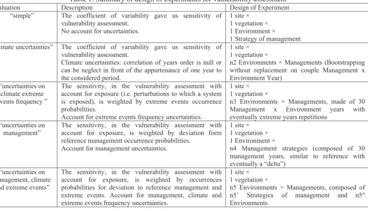
enough accuracy. Otherwise, we could account for uncertainties of one or many model-forcing components. In fact, we could define a whole set of approaches depending on released degrees of freedom. All these approaches are summed up into Table 1. To illustrate the different approaches, we will consider a simple case: a permanent pasture with a well known climate (30 years of weather data) and a known (and similar in time) management. We will only consider possible uncertainties on climate and management.

Table 1. Summary of design of experiments for vulnerability assessment

Evaluation Description Design of Experiment

“simple” The coefficient of variability gave us sensitivity of vulnerability assessment.

No account for uncertainties.

1 site × 1 vegetation × 1 Environment × 1 Strategy of management “climate uncertainties” The coefficient of variability gave us sensitivity of

vulnerability assessment.

Climate uncertainties: correlation of years order is null or can be neglect in front of the appurtenance of one year to the considered period.

1 site × 1 vegetation ×

n2 Environments × Managements (Bootstrapping without replacement on couple Management x Environment Year)

“uncertainties on climate extreme events frequency ”

The sensitivity, in the vulnerability assessment with account for exposure (i.e. perturbations to which a system is exposed), is weighted by extreme events occurrence probabilities.

Account for extreme events frequency uncertainties.

1 site × 1 vegetation ×

n3 Environments × Managements, made of 30 Management x Environment years with eventually extreme years repetitions

“uncertainties on management”

The sensitivity, in the vulnerability assessment with account for exposure, is weighted by deviation form reference management occurrence probabilities.

Account for management uncertainties.

1 site × 1 vegetation × 1 Environment ×

n4 Management strategies (composed of 30 management years, similar to reference with eventually a “delta”)

“uncertainties on management, climate

and extreme events”

The sensitivity, in the vulnerability assessment with account for exposure, is weighted by occurrences probabilities for deviation to reference management and extreme events. Account for management, climate and extreme events frequency uncertainties.

1 site × 1 vegetation ×

n5 Environments × Managements, composed of n5’ Strategies of management and n5" Environments

“Simple” evaluation

The first case consists in simply simulating the system over 30 years. The coefficient of variability (CV) will be taken as measure of sensitivity, needed for vulnerability assessment. As every year is considered as equiprobable, CV will allow us to calculate vulnerability while also accounting for exposure to climate variability. This first approach does not account for any kind of uncertainties. The DOE model is simple (Figure 4), as each factor (element of the ModVege metamodel input) only appears once. This approach allows a “simple” evaluation of the climate change impacts and its associated vulnerability.

Figure 4. Design of experiment model for “simple” evaluation of the vulnerability to climate change

Evaluation with account for climatic uncertainties In this case, we consider that climatic years are representative of a period, and that correlation between realizations at year N and year N-1 are negligible compared to the correlation of theses years and their membership to the period. So, we could consider that the order of occurrence of individual years is random. This is without any consideration for the fact that atmospheric CO2

increases over year. We could generate them by bootstrapping (sampling without replacement, e.g. Efron 1993), thus keeping climate realizations paired with management practices. As before, coefficient of variability can be used to evaluate sensitivity in the vulnerability assessment.

The resulting DOE (Figure 5) is, in this case, composed of fixed factors (Site and Vegetation) and of many Management strategies and Environments, which are composed of 30 realizations (without repetitions) of respectively Management Year and Environment Year. Due to the uniqueness of the constraint defined by the pair Management x Environment year, the latter has only 30 occurrences. The interest of this design is that it only takes into account part of the climate uncertainties.

Figure 5. DOE model for vulnerability assessment under climate change when accounting for climatic uncertainties

Evaluation with climate extreme events frequency uncertainties

Now, we suppose that in the initial climatic set, extreme events (EE) frequency could be higher than observed. So, we will simulate 30-year series, in which we will replace one or more years by an EE year. For the vulnerability assessment, it will be necessary to weigh up the relevance of the occurrence probability of extreme events in the climate series. For example, let’s suppose that the observed series contains one EE year, we could consider that the occurrence probability of the observed series is 50%, that the probability for the set of series with one more EE year (i.e. two EE years on 30 years) is 40%, and 9% and 1% for the series with two and three more EE years (i.e. three and four EE years on 30-year series, respectively).

Figure 6. DOE model for vulnerability assessment under climate change when accounting for uncertainties on extreme climate event frequency

The DOE (Figure 6) is made of two fixed elements: Site and Vegetation. The main differences with the previous DOE (Figure 5) are the cardinalities of yearly realizations.

Indeed, Management strategies and Environments are still composed of 30 years but some years can be repeated. In this DOE, we must differentiate “Normal” years from “Extreme” years, which can replace normal years. The interest of this DOE is that it accounts for uncertainties on EE frequency.

Evaluation with account for management uncertainties Another possibility could be to consider that the management could have been slightly different (for example, mowing dates slightly altered). In this case, we will use an experimental design testing the gap between new and initial dates. Thus, the first cutting date of the first year can be moved one week earlier, whereas the first cutting date of the second year is three days later, and so on. For the vulnerability assessment, we can estimate vulnerability, while accounting for exposure, by considering that the gap of days follows a known distribution (Gaussian for example). The DOE (Figure 7) is this time made of three fixed components (Site, Vegetation, Environment) and a set of Management strategies, which are in turn made of 30 Management years in which we can distinguish years similar to observation (Base) and those with a modification (With delta). This vulnerability assessment DOE allows accounting for management uncertainties.

Figure 7. DOE model for vulnerability assessment under climate change when accounting for management uncertainties

Evaluation with uncertainties on management and climate (including climate extremes)

To take into account all uncertainties and having a sensitivity evaluation, we could combine the three previous approaches. The main issue is the DOE size. A Latin Hypercube Design could be a suitable way to reduce the number of needed simulations

(

priori knowledge for the response surface and for

vulnerability assessment. In this DOE, we find a combination of Management Strategy and Environment. These are made of 30 elements, possibly with repetitions.

Figure 8. UML DOE Model for vulnerability assessment under climate change, accounting for uncertainties on management, climate including extreme events

Evaluation of vulnerability minimum

Once response surfaces will be fitted, a vulnerability minimum will be searched for. But, in fact, what we are really looking for is more a robust solution to reduce vulnerability than an optimal solution by a mathematically-suited fit. Indeed, due to the high environment uncertainties level, an optimal solution could completely fail (Kleijnen et al. 2005). Robust solutions should be in fact satisfactory with respect to vulnerability. For example, a robust solution should provide high grassland yield with low sensitivity to environment (that is, high stability); it should have by the way low vulnerability. An example of robust design, inspired by Taguchi (1987) can be found in Sanchez et al. (1996) and Kleijen and Gaury (2003). The evaluation of the found vulnerability will have two aims: firstly, we have to check that we really found a minimum of vulnerability and, secondly, we need to perform sensitivity analysis to evaluate the robustness of the solution. Finally, the DOE needed for this step will be similar to the DOE previously described (Figure 8).

METAMODEL OF IMPACT MODELS WITH ASSOCIATED DOE FOR VULNERABILITY ASSESSMENT

Figure 9. UML metamodel of agro-ecological model

Considering the DOE models we have previously proposed, we can identify a common pattern (Figure 9 and Figure 10).

Indeed, all Agro-ecological models use a set of Inputs, in which we can distinguish two types. On one hand, the Decision inputs are those who help applying a management strategy impacting results, and which must be optimised in function of the study criteria. On the other hand, the Environment inputs only bring uncertainties.

This distinction between these two types of inputs corresponds to Taguchi’s approach (Taguchi 1987). This classification is helpful to propose a metamodel in the MDE context (Bézivin 2005), which all agro-ecological model inputs would be conform to. We could also notice that there is a relationship linking the Inputs. This information is contained in the Constraint class, and it could also be specified mathematically:

“Let fT : D ĺ D’ be the characteristic function of a type of experimental design T, where D = D1xD2x…xDN is the domain of definition of the N inputs and

D’ = D’₁xD’₂x…xD’_{N the target domain of the function fT.}

D’ _{contains the set of factor level combinations ranged by}

the experimental design T.”

Figure 10. Instance diagram corresponding to a UML metamodel of DOE associated to an agro-ecological model. All DOE are compositions of Input instances, forming itself a set (class Input 1 x 2 x … x N).

Moreover, all DOE are the instance composition of Inputs (element 1, element 2 … element N). Those inputs can be combined (depending on the type of experimental design T) to create a set of inputs (Input 1 x 2 x … x N). All these inputs are constrained by instances of Constraint classes. They could be specified more accurately thanks to the OCL (“Object Constraint Language”, OMG 2010). OCL is a formal language to specify constraints between elements of UML graphs. The resulting cardinality (cardT) of the set of

inputs is a direct function of the DOE type. For example, if the design is a full factorial design then:

∏

Where cardi is the cardinality of input i instance definition

domain; we could notice that, in this special case, fT is in

fact the Identity function. If the design is a “One factor At a Time” (Kleijnen 1987), then:

¦

All DOE are conform to that representation.

All the examples of DOE we have presented are suitable for deterministic models. In the case of stochastic models, the approach will stay almost the same. A slight difference exists to add the replications of simulations in the DoE. It will also be necessary to account for noise into the response surface. Still in the case of stochastic DoE, it is interesting to specify the pseudo-random number generator in use and also to vary this generator among a set of reliable ones (Mersenne Twister series, WELLs and the latest MRGs from L’Ecuyer) (Hill 2010). The initialization and parallelization techniques of the random number generator do also have to be specified in high quality DOE.

DISCUSSION AND POSSIBLE SOLUTIONS

Vulnerability assessment is based on sensitivity analysis. Depending on the chosen definition, it can include the notion of exposure (by, for example, weighting years with extreme events). But it could also account for adaptations (limited by its real capacity). Identification and evaluation of adaptation options need a lot of simulations. In order to reduce this number (and mainly the computation time), we intend to use response surfaces instead of real simulations, for vulnerability minimum searching. Indeed, response surface can be used as model of simulations with a rather good accuracy and a faster computation time. Whatever the chosen definition and method, this requires a large number of simulations. Facing this issue, the choice of pertinent experimental designs appears as much critical as the simulation distribution question. Indeed, a suitable DOE will allow us to reduce the number of experiments as much as possible, whereas distribution to multiple computing platforms (i.e. clusters, grid, cloud computing) will reduce the waiting time to get all the results. We have already tackled the design of such software tools, which provide distributed computation and platform independent DOE (Amblard et al, 2003; Reuillon et al, 2008; Reuillon et al, 2010). However, theses tools do not take into account vulnerability assessments, in their actual state. To adapt them, we will need metamodels of the agro-ecological model and of the associated design of experiment.

CONCLUSION

Many simulations are necessary to perform a vulnerability assessment. We have defined different designs depending on the uncertainty levels that we wish to account for. For each of these designs, we have proposed a model. The study of the obtained models enabled us to go one step further with the proposition of a metamodel of agro-ecological models with their associated DOE. Each of the previously proposed models is conform to this metamodel. This work, following a reverse engineering experience (Lardy et al. 2011), can be seen as preliminary to build up a dedicated software framework for vulnerability assessment under climate change scenarios. This framework will tackle distribution of constrained experimental designs. We consider that a Model Driven Engineering approach will help us in the design and production of our future framework. The different models, according to the released degrees of freedom, and the associated metamodels

presented in this paper enable establishing the first step towards the design of a generic tool for climate change vulnerability assessment.

ACKNOWLEDGEMENTS

This work was jointly supported by the EC FP7 ‘GHG-Europe IP’ and the FP7 EU ‘CARBO-Extreme’ project.

REFERENCES

Amblard, F. Hill, D.R.C. Bernard, S. Truffot, J. Deffuant, G. 2003. “MDA Compliant Design of SimExplorer A Software Tool to Handle Simulation Experimental Frameworks”. Summer Computer Simulation Conference, Montreal, Canada, 279-284.

Atkinson, C. and Kuhne, T. 2003. “Model-driven development: a metamodeling foundation”. IEEE Software, 20, No.5, 36–41.

Bézivin, J. 2004. “In Search of Basic Principle for Model Driven Engineering”. Novatica Journal, Special Issue, March-April, No.2, 21-24

Bezivin, J. 2005. “On the unification power of models”.

Software and Systems Modeling, 4, No.2,171–188.

Carrère, P. Force, C. Soussana, J.-F. Louault, F. Dumont, B. and Baumont, R. 2002. “Design of a spatial model of perennial grassland grazed by a herd of ruminants: the vegetation sub-model”. Grassland Science in Europe, No.7, 282–283.

Downing, T.E. and Patwardhan, A. 2005. ”Assessing Vulnerability for Climate Adaptation”.. Adaptation Policy

Frameworks for Climate Change. Cambridge: Cambridge

University Press, pp. 67-89.

Easterling, W.E., Aggarwal, P.K., Batima, P., Brander, K.M., Erda, L., Howden, S.M., Kirilenko, A., Morton, J., Soussana, J.-F., Schmidhuber, J., Tubiello, F.N., 2007.

Food, fibre and forest products. Climate Change 2007: Impacts, Adaptation and Vulnerability. Contribution of Working Group II to the Fourth Assessment Report of the Intergovernmental Panel on Climate Change. Cambridge

University Press, Cambridge, United Kingdom, 273-313. Efron, B. 1993. An introduction to the bootstrap. Chapman &

Hall/CRC.

Favre, J-M., 2004. “Towards a basic Theory to Model Driven Engineering”. 3rd Workshop in Software Model

Engineering, WiSME 2004, 8p.

Favre, J-M, Estublier, J. Blay-Fornarino, M. 2006.

L’ingénierie dirigée par les modèles : Au delà du mda,

traité ic2, série informatique et systèmes d'information, Lavoisier, 227 p.

Füssel, H.-M., 2007. “Vulnerability: a generally applicable conceptual framework for climate change research”.

Global Environmental Change, No. 17, 155-167.

Füssel, H.M. Klein R. 2006. “Climate change vulnerability assessments: an evolution of conceptual thinking”.

Climatic Change, No.75, 301–329.

Graux, A.-I. Bellocchi G. Lardy R. Soussana J.-F. 2011. “Ensemble modelling of climate change risks and opportunities for managed grasslands in France”.

Agriculture and Forest Meteorology (submitted).

Hill, D.R.C., 1996. Object-oriented Analysis and Simulation. Addisson-Wesley, 291 pages.

Hill D.R.C., 2010, “Practical Distribution of Random Streams for Stochastic High Performance Computing”, Invited Paper in IEEE, International Conference on High

Performance Computing & Simulation (HPCS 2010),

Caen, June 28 – July 2, pp. 1-8.

Iacob, M. Steen, M. Heerink, L. 2008 “Reusable Model Transformation Patterns”. Workshop on Models and

Model-driven Method for Enterprise Computing (3M4EC

2008), pp 1-10.

IPCC (Intergovernmental Panel on Climate Change), 2001.

Impacts, adaptation, and vulnerability climate change 2001. Third Assessment Report of the IPCC.

UniversityPress, Cambridge, UK. 1032 p.

Jouven, M. Carrere, P. Baumont, R. 2006a. “Model predicting dynamics of biomass, structure and digestibility of herbage in managed permanent pastures. 1. Model description”. Grass and Forage Science, No.61, 112-124. Jouven, M. Carrere, P. Baumont, R. 2006b. “Model predicting

dynamics of biomass, structure and digestibility of herbage in managed permanent pastures. 2. Model evaluation”. Grass and Forage Science, No.61, 125-133. Kasperson J.X. Kasperson R.E. Turner II B.L. Schiller A.

Hsieh W.-H. 2005. “Vulnerability to global environmental

change”. The Human Dimensions of Global

Environmental Change. Rosa, E. A., Diekmann, A., Dietz,

T., Jaeger, C.C. (eds.) MIT Press, Cambridge MA. Kempthorne O. 1952. The Design and Analysis of

Experiments. Wiley, Publications in Statistics, 631 p.

Kleijnen, J.P.C. 1987. Statistical tools for simulation

practitioners. New York: Marcel Dekker, 429 p.

Kleijnen, J. P. C. Gaury E. 2003. “Short-term robustness of production management systems: A case study”. European

Journal of Operation Research. No.148, 452–465.

Kleijnen, J.P.C. Sanchez, S.M. Lucas, T.W. and Cioppa, T.M. 2005. “State-of-the-Art Review: A user's guide to the brave new world of designing simulation experiments”.

INFORMS Journal on Computing, 17, No.3, pp. 263-289

Kleppe, A. Warmer, S. Bast, W. 2003. “MDA Explained The Model Driven Architecture: Practice and Promise”, Addison-Wesley. 1992 p.

Lano, K. Clark, D. 2008. “Model Transformation Specification and Verification”. The Eighth International

Conference on Quality Software. QSIC’08. 45-54.

Lardy, R. Graux, A.-I. Gaurut, M. Bellocchi, G, Hill D.R.C. 2011. “Model Driven Reverse Engineering For A Grassland Model With Design Of Experiment In The Context Of Climate Change”, The SummerSim’11 The Hague, 27-29 June, CD proceedings 8 p.

Louault, F. Pillar, V.D. Aufrère, J. Garnier, E. and Soussana, J.-F. 2005. “Plant traits and functional types in response to reduced disturbance in semi-natural grassland”. Journal of Vegetation Science, No.16, 151– 160.

Luers, A.L., Lobell, D.B., Sklar, L.S., Addams, C.L., Matson, P.A., 2003. “A method for quantifying vulnerability, applied to the agricultural system of the Yaqui Valley, Mexico”. Global Environmental Change, No.13, 255-267. McKay, M. D., Beckman, R. J., Conover, W. J., 1979. “A

comparison of three methods for selecting values of input variables in the analysis of output from a computer code”.

Technometrics No.21, 239-245.

OMG, 2002. “Meta Object Facility (MOF) Specification” Version 1.4, April.

OMG (Object Management Group), 2010. "Object Constraint Language, Version 2.2, February 2010", http://www.omg.org/spec/OCL/2.2.

Rahim, L. And Mansoor, S. 2008. “Proposed Design Notation for Model Transformation”. 19th Australian Conference on Software Engineering, ASWEC 2008, 589-598. Reuillon, R., Chuffart, V., Leclaire, M., Faure, T., Dumoulin,

N., and Hill, D.R.C., 2010, “Declarative task delegation in OpenMole”. In proceedings of International Conference

on High Performance Computing and Simulation, Caen,

June 28 – July 2, pp. 55-62.

Reuillon, R., Hill, D.R.C., El Bitar, Z. And Breton, V., 2008. “Rigorous distribution of stochastic simulations using the

DistMe toolkit”, IEEE Transactions On Nuclear Science, Vol. 55, No. 1, February, pp. 595-603.

Sanchez, S. M. Sanchez P. J. Ramberg J. S. Moeeni F. 1996. “Effective engineering design through simulation”. International Transaction in Operational Research No.3,169–185.

Seidewitz, E. And Technologies, I. 2003. “What models mean”. Software, IEEE, 20, No.5, 26-32.

Taguchi, G. 1987. System of experimental designs, volumes 1

and 2. UNIPUB/ Krauss International, White Plains, New

York.

Thornley, J.H.M. 1998. Grassland dynamics. An ecosystem

simulation model, CAB International, Wallingford, United

Kingdom, 256 p.

Turner B.L. II, Kasperson R.E. Matson P.A. Mccarthy J.J. Corell R.W. Christensen L. Eckley N. Kasperson J.X. Luers A. Martello, M.L. Polsky C. Pulsipher, A. Schiller A. 2003. “A framework for vulnerability analysis in sustainability science”. Proceedings of the National

Academy of Sciences of the United States of America

Vol.100, No.14, July, 8074–8079.

Volenec, J.J. Ourry, A. and Joern, B.C. 1996. “A role for nitrogen reserves in forage regrowth and stress tolerance”.

Physiologia Plantarum, No.97, 185–193.

BIOGRAPHIE

ROMAIN LARDY is a PhD student jointly at the LIMOS (ISIMA) - UMR CNRS 6158 of Blaise Pascal University of Clermont Ferrand (France), and at the UREP in the French National Institute for Agricultural Research (INRA). His work is focused on High Performance Vulnerability Assessment with constrained Design of Experiments using a model driven engineering approach, applied to climate change vulnerability of grassland / livestock systems.

GIANNI BELLOCCHI is a senior scientist at the Grassland Ecosystem Research Unit (UREP), of the French National Institute for Agricultural Research (INRA) at Clermont-Ferrand. He has co-authored many scientific papers related to agronomy, plant physiology and climatology. His current research aims at enhancing the use of modelling tools to analyze grassland/livestock systems under climate change.

BRUNO BACHELET is Associate Professor at Blaise Pascal University. He received a Ph.D. degree from Blaise Pascal University in 2003. His current work is focused on software engineering techniques for scientific computing, mainly for operations research applications and simulation models.

DAVID HILL is currently Vice President and Professor at Blaise Pascal University. Since 1990, Professor Hill has authored or co-authored many technical papers and journal papers and he has published various text books including recent free e-books from Blaise Pascal University Press (http://www.isima.fr/~hill)