HAL Id: halshs-00607748
https://halshs.archives-ouvertes.fr/halshs-00607748v2
Preprint submitted on 13 Jul 2011
HAL is a multi-disciplinary open access archive for the deposit and dissemination of sci-entific research documents, whether they are pub-lished or not. The documents may come from teaching and research institutions in France or abroad, or from public or private research centers.
L’archive ouverte pluridisciplinaire HAL, est destinée au dépôt et à la diffusion de documents scientifiques de niveau recherche, publiés ou non, émanant des établissements d’enseignement et de recherche français ou étrangers, des laboratoires publics ou privés.
How Wages and Employment Adjust to Trade
Liberalization: Quasi-Experimental Evidence from
Austria
Marius Brülhart, Céline Carrere, Federico Trionfetti
To cite this version:
Marius Brülhart, Céline Carrere, Federico Trionfetti. How Wages and Employment Adjust to Trade Liberalization: Quasi-Experimental Evidence from Austria. 2011. �halshs-00607748v2�
1
GREQAM
Groupement de Recherche en Economie Quantitative d'Aix-Marseille - UMR-CNRS 6579 Ecole des Hautes études en Sciences Sociales
Universités d'Aix-Marseille II et III
Document de Travail
n°2011-33
How Wages and Employment Adjust to
Trade Liberalization: Quasi-Experimental
Evidence from Austria
Marius Brülhart
Céline Carrère
Federico Trionfetti
How Wages and Employment Adjust to Trade Liberalization:
Quasi-Experimental Evidence from Austria
Marius Brülhartz
University of Lausanne
Céline Carrèrex
University of Geneva
Federico Trionfetti{
GREQAM, Université de la Méditerranée June 2011
Abstract
We study the response of regional employment and nominal wages to trade liberaliza-tion, exploiting the natural experiment provided by the opening of Central and Eastern European markets after the fall of the Iron Curtain in 1990. Using data for Austrian municipalities, we examine di¤erential pre- and post-1990 wage and employment growth rates between regions bordering the formerly communist economies and interior regions. If the ‘border regions’are de…ned narrowly, within a band of less than 50 kilometers, we can identify statistically signi…cant liberalization e¤ects on both employment and wages. While wages responded earlier than employment, the employment e¤ect over the entire adjustment period is estimated to be around three times as large as the wage e¤ect. The implied slope of the regional labor supply curve can be replicated in an economic geog-raphy model that features obstacles to labor migration due to immobile housing and to heterogeneous locational preferences.
JEL Classi…cation: F15, R11, R12
Keywords: trade liberalization, spatial adjustment, regional labor supply, natural ex-periment
<All tables and …gures at end>
We thank Robert Staiger and Daniel Sturm for helpful suggestions; Josef Zweimüller, Rafael Lalive, Oliver Ruf, Eva Ortner and Gudrun Bif‡ for facilitating our access to the data; and seminar participants at the Graduate Institute of International and Development Studies, Geneva, the London School of Economics, the Paris School of Economics, the Universities of Innsbruck, Lausanne, Namur and Utrecht, and at the 2009 conference of the Urban Economics Association, San Francisco, for valuable comments. Nicole Mathys has provided excellent research assistance. We gratefully acknowledge …nancial support from the Swiss National Science Foundation (NCCR Trade Regulation, and grants 100012-1139938 and PDFMP1-123133) and from the EU 6th Framework Programme (“Micro-Dyn” project).
zDepartment of Economics (DEEP), Faculty of Business and Economics, University of Lausanne, 1015
Lau-sanne, Switzerland (Marius.Brulhart@unil.ch). Also a¢ liated with the Centre for Economic Policy Research (CEPR), London.
xEuropean Institute, University of Geneva, 1204 Geneva, Switzerland (celine.carrere@unige.ch).
{GREQAM, Château La Farge, Route des Milles, 13290 Les Milles, France
1
Introduction
We address a fundamental but to date surprisingly underresearched question: how do changes in market access a¤ect factor prices and factor quantities? To put it simply: if a certain region o¤ers advantageous access to markets elsewhere, will this advantage translate into a large number of producers locating in that region, will it translate into higher factor rewards for producers located there, or will we observe some of both e¤ects? As a natural corollary to this question, we also study such e¤ects across di¤erent time horizons, as quantity and price adjustments may well materialize at di¤erent speeds. We focus on the case where changes in market access are due to the liberalization of international trade.
Why should we care about the di¤erence between factor price e¤ects and factor quantity e¤ects of changes in market access? First, this distinction helps us understand adjustment mechanisms of regional economies, by allowing us to trace regional factor supply schedules. For example, large price e¤ects suggest the existence of important barriers to the reallocation of labor and capital across space and/or across sectors. Information on the relative magnitude of price and quantity e¤ects can thereby help us gauge the realism of alternative theoretical models. Second, the policy implications of market-access e¤ects vary considerably depending on whether these e¤ects work through factor prices or through factor quantities. Price e¤ects bring about spatial inequality of (pre-tax) factor rewards, which can potentially be evened out via redistributive policy. Quantity e¤ects may imply problems from congestion in central locations and depopulation in peripheral ones, or from specialization patterns that make regions vulnerable to sector-speci…c shocks.
Almost all research to date has focused on the two polar cases, by looking either at quantity e¤ects or at price e¤ects, thus implicitly assuming regional factor supply schedules to be either horizontal or vertical. Many empirical studies that are formally linked to the theory assume that intersectoral and/or interregional factor supplies are in…nitely elastic, which leaves room for quantity e¤ects only. The sizeable empirical literature on home-market e¤ects, initiated by Davis and Weinstein (1999), belongs to this category. Redding and Sturm (2008) were …rst to explore quantity adjustment using a natural experiment involving changes in market access, by tracking changing populations of cities located along the border between East and West Germany during the country’s division and reuni…cation in the 20th century. Faber (2009) has studied the e¤ects of highway construction in China on industrial production of
rural counties to identify the causal e¤ect of market access on regional output. Conversely, a strand of the literature due mainly to Hanson (1997, 2005) has assumed that factor supplies are inelastic, such that market-access e¤ects manifest themselves solely via factor prices (i.e. wages). Redding and Venables (2004) have used this approach to study the determinants of international di¤erences in per-capita income and found that the geography of access to markets and sources of supply is quantitatively important.
When speci…cally studying intra-national adjustment to international trade liberalization, most researchers have looked at quantity e¤ects, mainly in terms of city populations (e.g. Ades and Glaeser, 1995; Henderson, 2003) and of regional employment (e.g. Hanson, 1998; Brülhart, Crozet and Koenig, 2004; Sanguinetti and Volpe Martincus, 2009). A smaller number of researchers have alternatively considered price e¤ects, in terms of regional wages (e.g. Hanson, 1997; Chiquiar, 2008). The combination of quantity and price e¤ects has not yet, to our knowledge, been studied in this context.
The theoretical distinction between price and quantity e¤ects of market access has been brought into focus by Head and Mayer (2004). Using a economic geography model featuring imperfectly elastic factor supply to the sector that is subject to agglomeration forces, they showed that, depending on the size of this elasticity, quantity e¤ects or price e¤ects may dominate. In a subsequent paper (Head and Mayer, 2006), they have investigated this issue empirically, by estimating how European region-sector wages deviate from a benchmark pat-tern that would be consistent with pure quantity responses to agglomeration forces. They found stronger evidence for price e¤ects than for quantity e¤ects. They acknowledged that, while their strategy for estimating wage responses was fully structural, the estimation of em-ployment changes had to rely on ad hoc regressions, and that their empirical implementation faced considerable challenges in terms of measurement and causal inference.
Our approach is to draw on a natural experiment and to use a di¤erence-in-di¤erence identi…cation strategy. We take the fall of the Iron Curtain in 1990 as an exogenous event that increased overall market access of Austrian regions, but more so for regions close to Austria’s eastern border. Comparing post-1990 wage and employment growth in border regions to that in interior regions, we can control for common shocks and isolate the e¤ects of increased market access with considerable con…dence. This quasi-experimental strategy obviates the need to construct an arti…cial benchmark that would have to be tied to a speci…c variant of
the underlying model and would inevitably be prone to measurement error.
Our central contribution is to consider factor-price e¤ects as well as factor-quantity e¤ects. Speci…cally, we trace the impact of improved market access on both nominal wages and employment levels. We …nd that the employment e¤ect exceeds the wage e¤ect by a factor of around three. Furthermore, we are able to characterize the time pro…le of adjustment along those two margins, observing that wage rises precede the increases in employment.
In addition, we seek to replicate our estimated ratio of employment-to-wage-adjustment in a calibrated three-region economic geography model. A nontradable housing sector acts as a dispersion force against the agglomeration tendencies that arise from the interplay of trade costs, product di¤erentiation and increasing returns. When we add a further dispersion force due to heterogeneous locational preferences, we …nd that the model predicts our central estimate of relative labor-market adjustment margins for realistic parameter values.
The remainder of the paper is organized as follows. In Section 2, we present a theoretical model of regional adjustment to external trade liberalization. Section 3 describes the quasi-experimental empirical setting and the data. Our estimation strategy is described in Section 4, and empirical results are reported in Section 5. In Section 6, we examine the behavior of the theoretical model with a view to reproducing our key estimated parameter. Section 7 concludes.
2
Theory
2.1 A Three-Region Geography Model
Our theoretical starting point is the variant of Krugman’s (1991) “new economic geography” model proposed by Helpman (1998), which o¤ers an attractive framework for the analysis of market-access e¤ects at the region level, as it explicitly considers congestion costs due to a non-tradeable resource H, thought of as housing.1
Details of the model are given in the Appendix. Here, we focus on sketching its main elements.
The model features three regions, indexed by i: two regions in A(ustria) and one region
1Using this model will allow us to compare our results to those obtained by Redding and Sturm (2008).
In Section 6, we shall extend the Helpman model by introducing heterogeneous locational preferences as an additional dispersion force.
R(est of the world). A is composed of an interior region I and a border region B. Labor, L, the sole production factor, is assumed to be fully employed and perfectly mobile within A but immobile between A and R. Workers spend a fraction of their income on varieties of a di¤erentiated traded good, M , with a taste for variety represented by the substitution elasticity . The remaining fraction of income, 1 , is spent on housing H. The market for M is Dixit-Stiglitz monopolistically competitive. Individuals decide where to locate according to the indirect utility they obtain from consumption of M and H.
Our comparative-static exercise will consist of tracking changes in nominal wages and em-ployment within A as trade costs between A and R are lowered. We are interested in the parameter , the border region’s di¤erential change in employment relative to its di¤erential change in the nominal wage, induced by the fall in external trade costs. This elasticity repre-sents the slope of the regional labor supply curve. A high value of means that employment reacts strongly while nominal wages do not, implying a relatively elastic interregional labor supply; and vice-versa for a low value of . As our simulations will show, is not only a highly policy relevant variable but it also turns out to be robust to assumptions on trade costs and country sizes for which it is impossible to determine the “realistic” values.
The non-linearity of the model makes it algebraically unsolvable. We therefore resort to numerical simulations.2
2.2 The Experiment
As we seek to model external trade liberalization of an integrated country, we assume low trade costs within A, and we let trade costs between B and R decline from an almost prohibitive level to the same low level that we assume to exist within A.
Regions are separated by iceberg trade costs, such that for every unit sent from region i to region j only a fraction ij 2 (0; 1) arrives in j. The geographical structure of the three-region
model is represented by the following assumptions on trade costs:
2The Maple …les used for the simulations are available from the authors. The model can in principle imply
multiple and unstable equilibria. We have ascertained that the equilibria obtained for each set of parameter values are unique and stable. The uniqueness and stability condition for equilibria in the Helpman (1998) model
is (1 ) > 1. Some parameter combinations used in our simulations violate this condition. Nonetheless,
the equilibria we obtain turn out to be stable and unique. The reason is that, in our three-region version of the Helpman model, only a fraction of world demand is mobile (regional demand within A). Therefore, forces that favor instability are attenuated compared to the original two-region model. The extended version of this model (Section 6) is more stable still than the baseline model, since it contains an additional dispersion force in the form of taste heterogeneity.
IR = IB BR;
which means that for a unit of the M -good to be transported between I and R it has to transit through B. Thus, the border region is nearer to R than the interior region.
We choose the following parameter values to simulate external trade liberalization:
IB = 0:9;
BR = f0:1; 0:2; 0:3; 0:4; 0:5; 0:6; 0:7; 0:8; 0:9g :
We solve the model for each of the nine levels of BR, and we compute the percentage
change in equilibrium nominal wages, wi, and employment, Li, for each 0.1 increment of trade
cost reduction.3
We can then calculate the ratio between the di¤erence in growth rates of employment and the di¤erence in growth rates of wages:
LB LI
wB wI
:
This ratio is computed for every increment of trade-cost reduction, which yields eight such ratios for each combination of parameters other than ij. As we will show, it turns out that
varies only trivially across pairs of trade costs for which it is calculated. We will therefore report averages of the eight computed ratios.
To calibrate this model, we need to decide on the values of the following parameters: housing stocks (in each region), Hi, population in A and R, the elasticity of substitution
among di¤erentiated goods, , and the expenditure share of housing, 1 . The population distribution within A is, of course, endogenous.
In order to cover the range of recent empirical estimates of substitution elasticities, we experiment with values of in the interval from 3 to 6.4 As we shall see, the value assumed
3
wi and Li are percentage changes between steady states. To be clear, let w BR=0:1 and w BR=0:2
be equilibrium wages in B when BR = 0:1 and when BR = 0:2, respectively. Then wB =
w BR=0:2 w BR=0:1 =w BR=0:1, and analogously for wages in I and for employment. The empirical
coun-terparts are cumulative growth rates over the entire pre- and post-liberalization subperiods, assuming that these subperiods are su¢ ciently long to capture the full transition between steady states.
4
See, e.g., Baier and Bergstrand (2001), Bernard, Eaton, Jensen and Kortum (2003), Hanson (2005), Broda and Weinstein (2006) and Head and Mayer (2006).
for the housing share (1 ) is crucial. We take 0.25 as our best guess but shall explore the implications of alternative values. According to the OECD input-output table for Austria in 1995, housing expenditure amounted to 25 percent of the total wage bill and of 15 percent of the total wage bill plus net pro…ts.5 The distribution of housing stocks within A is obtained by calibrating the model so as to replicate the population distribution observed in our data.6 We exogenously assign a distribution of the total stock of housing between A and R, choosing HR= H3 and LR= L3 and normalizing total stock of housing and labor by setting H = L = 1.
Hence, A is twice the size of R. This is arbitrary, but, as we shall show in Section 6.1, the implied s are almost una¤ected by di¤erent parametrizations of HR and LR as well as to
di¤erent-sized changes in trade costs.
2.3 Simulation Results
Table 1 reports the simulated values of for several combinations of and (1 ). The values of this ratio range from 2.21 to 10.33. For what we consider our most realistic parameter combination, = 4 and (1 ) = 0:25, the predicted equals 7.16. This implies that the magnitude of trade-shock induced employment growth in the border region is some seven times larger than the magnitude of the trade-shock induced increase in nominal wages. At face value, this could be taken to suggest rather elastic interregional labor supply.
As a check on the robustness of this result, we report implied values of , and for di¤erent levels and changes of external trade costs and for di¤erent relative sizes of country A and the rest of the world B in Table 2. Inspection of the table shows that the implied wage and employment e¤ects are sensitive to these assumptions: the larger the cut in external trade costs, and the larger the size of the outside economy, the larger are the simulated values of and . This is why looking at these e¤ects themselves would be of little help in mapping the model to the data. When we focus on their ratio, however, this issue no longer arises, as turns out to be robust to modelling choices on variables other than and (1 ).7 This lack of sensitivity is not surprising. By increasing the size of R, for instance, trade liberalization
5
Davis and Ortalo-Magné (2011) …nd that, between 1980 and 2000, the median US household expenditure share of housing was a stable 0.24, with a standard deviation of 0.02.
6
In our data set, municipalities belonging to our baseline de…nition of the border region (B) accounted for 5.1 percent of Austrian population prior to liberalization. Their implied housing stock in our calibrations ranges from 6 to 9 percent of the total for country A.
7
In addition to the sensitivity analyses reported in Table 2, we have explored the implications of changing
the assumed intra-country trade cost IB:We found the simulated values of to be essentially insensitive to
becomes more important for both I and B, but more so for B. Yet, is not a measure of the locational attractiveness of B relative to I; rather, it captures whether that increased attractiveness manifests itself more in terms of employment growth or in terms of nominal wage growth. This ratio is largely insensitive to the overall attractiveness of B with respect to I.
We now turn to an empirical estimation of .
3
Empirical Setting and Data
3.1 Austria and Eastern Europe Before and After the Fall of the Iron Curtain
The experience of Austria over the last three decades provides a propitious setting, akin to a natural experiment, within which to explore regional responses to changes in trade openness. In 1975, at the beginning of the period covered by our study, Austria lay on the eastern edge of democratic, market-oriented Europe. By 2002, which marks the end of our sample period, it found itself at the geographical heart of a continent-wide market economy. We argue that the fall of the Iron Curtain can be thought of as an exogenous change in market access, that it was unanticipated, that it was large, and that it a¤ected di¤erent Austrian regions di¤erently. We assume that the lifting of the Iron Curtain was exogenous to events in Austria. More-over, during the period covered by our study, this transformation took the form of a trade shock: a large change in cross-border openness of goods markets with little concomitant change in openness to cross-border worker ‡ows.8
The timing of the main “exogenous shock” is also straightforward to pin down. While some economic reforms had started across communist Europe soon after the ascent of Mikhail Gorbachev in 1985, the rapid break-up of the Soviet bloc in 1989-90 took most contemporary
8Free East-West mobility of workers only started to be phased in after EU enlargement in 2004, well after
the end of our sample period. In a review of pre-enlargement migration patterns and policies, the OECD (2001) concluded that “except for Germany, the employment of nationals of the CEECs in OECD member countries did not increase signi…cantly [post-1990]” (p. 35) and that “the current state of integration between the CEECs and the EU is characterized by limited labour ‡ows but strong trade integration and increasing capital market integration”(p. 107). Austria had experienced considerable in‡ows of mainly …xed-term “guest workers”from Yugoslavia already before 1990. Available data from the WIFO’s “SOPEMI Reports”show that the number of Yugoslav and CEEC workers in Austria in fact shrank between 1992 and 2001, from 134,000 to 71,000 and from 42,000 to 38,000 respectively. The treatment we analyze can therefore be considered as a trade shock. For an analysis of a cross-border opening of labor markets, see Buettner and Rincke (2007), who used German reuni…cation as a quasi-experiment to explore the impact of migration on border-region employment and wages.
observers by surprise. In January 1989, the fact that a mere two years later all of Austria’s Comecon neighbors (Czechoslovakia, Hungary and Slovenia) as well as nearby Poland and even the Soviet Union itself would have held democratic elections and jettisoned most aspects of central planning, was unexpected by most.9 Hence, we de…ne 1990 as the watershed year that marked the general recognition of a lasting economic transformation of the Central and Eastern European countries (CEECs) and of their new potential as trade partners. Actual trade barriers, however, only fell gradually post-1990. The main milestones in this respect were the entries into force of free trade areas between the EU and Hungary, the Czech Republic, Slovakia and Poland in 1992, and with Slovenia in 1996.10 Furthermore, the Eastern European
countries all applied for full EU membership in the mid-1990s.11 Austria itself had lodged its membership application in 1989 and joined the EU in 1995. In short, the decade following 1990 was a period of gradual but profound and lasting mutual opening of markets, to an extent that up to the very late 1980s had been largely unanticipated.
The magnitude and time pro…le of the post-1990 transformation can be gleaned from Figure 1, where we report Austrian bilateral trade volumes with its neighboring countries, scaled relative to their 1990 values. The take-o¤ in 1990 of trade between Austria and its formerly communist neighboring countries is evident. While, over the 1990s, the share of Austria’s trade accounted for by its western neighbor countries shrank by between 13 percent (Germany) and 20 percent (Switzerland), it increased by 107 percent with Hungary and by 178 percent with the Czech and Slovak republics. Figure 1 shows that trade with the former constituent parts of Yugoslavia only took o¤ by the middle of the decade, which is unsurprising given the wars in Croatia and Bosnia-Herzegovina that lasted until 1995. Trade with Slovenia has been recorded separately since 1992. It shows a continuous increase as a share of Austrian trade of 78 percent between 1992 and 2002. The data thus con…rm that 1990 marked the start
9Some quotes from The Economist magazine illustrate this point. In its issue of 7 January 1989 (p. 27),
The Economist wrote of Gorbachev’s “chance to relaunch [his] reforms for the start of the next …ve-year plan in 1991” but warned that “real reform [...] may have to wait until the 1996-2000 plan”. The centrally planned economy was evidently expected to last at least for the rest of the decade. In its 11 March edition (p. 14), The Economist speculated about a possible loss of power by Gorbachev and concluded that “if there were a bust-up over reform, the regime that would replace Mr Gorbachev’s would probably be conservative, disciplinarian and much less interested in rejoining the world”. This shows that informed opinion in early 1989 considered a continuation of the gradual Gorbachev reforms as the most likely (or even only) path towards East-West integration - with a considerable risk of a restoration of hardline communist control and the attendant economic isolation. A sudden collapse of the communist system did not feature among the scenarios considered probable until the second half of 1989, in particular after the fall of the Berlin Wall on 9 November of that year.
1 0Formally, these are the starting dates of “Interim Agreements”. The o¢ cial “Europe Agreeements”entered
into force two to three years later. Trade barriers were phased out gradually over up to ten years, but
liberalization already started during the Interim Agreement period.
of a large and sustained eastward reorientation of Austrian trade.12
Austria’s small size implies that access to international markets is important: it was the OECD’s …fth most trade oriented country in 1990.13 Moreover, simple inspection of a map reveals that the transformations in Austria’s eastern neighbors should have a¤ected Austrian regions with di¤erent intensity (see Figure 2). Austria’s east-west elongated shape accentuates the fact that access to the eastern markets becomes relatively less important than access to western markets as one crosses Austria from east to west. Regional trade data would allow us to corroborate this claim explicitly. No such statistics exist for Austria, but there is strong evidence from other countries of gravity-type trade patterns also at the sub-national level.14
Furthermore, we can draw on region-level data on foreign direct investment (FDI) collected by the Austrian central bank. In Figure 2, we report the CEEC share of the stock of outward FDI projects by Austrian …rms. This map shows that …rms in eastern Austria are signi…cantly more oriented towards the eastern European markets than …rms based in western Austria, and that this gradient has remained just as strong in 2002 as it was in 1989. The FDI data corroborate the trade data in showing how strongly the Austrian economy turned eastwards post-1990: the share of Austrian FDI projects hosted by CEECs rose from 14 percent of total Austrian FDI in 1989 to 51 percent in 2002. In 2002, a full 96 percent of FDI from Austria’s most easterly region (Burgenland) was targeted at CEECs, while the corresponding share of Austria’s most westerly region (Vorarlberg) was 23 percent. Austria thus provides us with considerable variation for identifying e¤ects that are speci…cally due to improved access to eastern markets.
As we couch our analysis within a market-based model of spatial wage and employment adjustments, we need to ascertain that such a model is indeed appropriate for our empirical setting. Almost all Austrian …rms are bound by industry-level collective wage agreements. These agreements allow for some regional di¤erentiation. More important, however, is the fact that the agreed rates serve as wage ‡oors that are rarely binding and thus allow for considerable ‡exibility across …rms and regions. In 2001, for example, the average agreed
1 2
The geographic reorientation of Austrian trade occurred against a background of steadily increasing overall trade orientation. Imports and exports corresponded to 58 percent of Austria’s GDP in 1975, to 73 percent in 1989 and to 93 percent in 2002 (OECD data). This was a faster expansion than the OECD average (1975 de…nition): Austrian trade accounted for 1.43 percent of OECD trade in 1975, for 1.59 percent in 1989 and for 1.80 percent in 2002.
1 3Only Luxembourg, Belgium, Ireland and the Netherlands had higher trade-to-GDP ratios.
1 4
See, for example, Combes, Lafourcade and Mayer (2005) and Helble (2007) for Europe, and Hillberry and Hummels (2003, 2008) for the United States.
wage rate in the highest-wage region (Vorarlberg) exceeded that of the lowest-wage region (Burgenland) by 17 percent, and the corresponding di¤erence in average e¤ective wage rates amounted to fully 36 percent.15 Another piece of evidence of relatively ‡exible private-sector wage setting in Austria is given by Dickens et al. (2007), who show that in a sample of 16 industrialized countries, Austria has the seventhlowest downward rigidity of nominal wages -somewhat more rigid than the UK, but -somewhat less rigid than Germany and considerably less so than the United States. We conclude that Austria provides an appropriate setting for our analysis also in terms of the structure of its labor market.
3.2 A Data Set on Wages and Employment in Austrian Municipalities
Our analysis is based region-level measures of employment and wages computed from the Austrian Social Security Database (ASSD). The ASSD records individual labor-market histo-ries, including wages, for the universe of Austrian workers.16 These records can be matched
to establishments, which allows us to allocate workers to locations. We observe wages and employment at three-month intervals, taken at the mid point of each quarter, yielding 112 measurements from the …rst quarter of 1975 to the fourth quarter of 2002.
The wage data are right censored, because social security contributions are capped at a level that is adjusted annually, and e¤ective income exceeding that limit is not recorded. In order to minimize distortions from such censoring, we construct wages as medians across individuals by municipality.17 Wages are recorded on a per-day basis, which means that they are broadly comparable irrespective of whether employment contracts are part-time or full-time.
The ASSD assigns each establishment to one of 2,305 municipalities. Our identi…cation strategy will hinge on the relative distances of these municipalities to eastern markets. Our main measure is the road distance to the nearest border crossing to one of Austria’s formerly communist neighbor countries. As an alternative, we use the shortest road travel time be-tween each municipality and the nearest eastern border crossing, computed as road distances
1 5
These data are taken from the 2002 statistical yearbook of the Austrian Federal Economic Chamber.
1 6For a thorough description, see Zweimüller et al. (2009). Public-sector workers are not covered by this
database prior to 1988, nor are the self-employed. We therefore work exclusively with data pertaining to private-sector employees.
1 7
A comparison of annual median wages (reported by Statistics Austria) to the censoring bounds in the ASSD (reported by Zweimüller et al., 2009), shows that the former falls very comfortably between the latter in all our sample years.
weighted by average traveling speeds.18 Since we can allocate …rms to one of 16 sectors, we can furthermore control for the industrial composition of municipalities.19
4
Estimation Strategy
Our basic estimation strategy follows the di¤erence-in-di¤erence approach applied by Redding and Sturm (2008). We regress the endogenous variable of interest on the interaction between a dummy for border regions (Border) and a dummy that is equal to one for all years from 1990 onwards (F all), as well as on a full set of time (t) and location (i) …xed e¤ects. The coe¢ cient estimated on the interaction term measures whether and how the dependent variable evolved di¤erently in border regions (the treatment group) compared to interior regions (the control group) after the fall of the Iron Curtain.
Speci…cally, we estimate the following equation for median nominal wage growth:
W ageit= (Borderi F allt) + di+ dt+ "wageit ; (1)
where, in our baseline speci…cation, W ageit is the annual growth rate measured at
quarterly intervals:
W ageit=
W ageit W ageit 4
[W ageit+ W ageit 4] 0:5
;
di denotes a full set of municipality …xed e¤ects, dt denotes a full set of quarter …xed
e¤ects, and "wageit is a stochastic term. Unobserved time-invariant heterogeneity in municipal wage levels is di¤erenced out by taking growth rates. Furthermore, the municipality-speci…c dummies control for any unexplained di¤erences in linear wage trends, and the time dummies control for nation-wide temporary shocks to median wage levels including the common impact of the fall of the Iron Curtain on median wages across all of Austria.20
We then apply a corresponding speci…cation for changes in municipal employment:
1 8Road distances and travel times were obtained from Digital Data Services GmbH, Karlsruhe, Germany.
These data pertain to measurements taken in the early 1990s. While some cross-border roads have been upgraded after 1990, we are not aware of any signi…cant new border crossings that have been constructed between 1990 and 2002, except for a highway link with Slovenia that was opened in 1991.
1 9The list of sectors covers the full spectrum of economic activities and primarily consists of aggregates of
NACE two-digit industries (see Zweimüller et al., 2009).
2 0
Emplit= (Borderi F allt) + di+ dt+ "emplit ; (2)
where Empl is de…ned equivalently to W age.
In an alternative speci…cation, we express Empl and W age as changes over the full pre- and post-1990 sample periods.
Our coe¢ cients of interest areb and b. They capture the di¤erential post-1990 trajectories of nominal wages and employment in border regions, which we interpret as the e¤ect of increased market access subsequent to the fall of the Iron Curtain.
The ratio of the two coe¢ cients, b = bb, provides us with a measure of the relative magnitudes of employment and nominal wage adjustments, and thus of the slope of the average municipal labor supply curve, which we can compare to the value predicted by theory.21
As a complement to parametric estimation, we report non-parametric evidence on the relationship between, on the one hand, the growth of median wages or total employment in each municipality and, on the other hand, the distance of the respective municipalities to the eastern border. Speci…cally, we estimate the following equations:
W ageit = i(F allt di) + di+ dt+ !wageit ; and (3)
Emplit= i(F allt di) + di+ dt+ !emplit : (4)
The parameters bi and bi represent municipality-speci…c estimates of di¤erential average
growth after 1990 compared to the pre-1990 period. A plot of the relationship between these parameters and municipalities’distance to the eastern border can give us an indication of the market-access e¤ect without any prior restriction on the de…nition of the treatment sample (i.e. of “border” municipalities).
Speci…cations (1) and (2) allow us to estimate treatment e¤ects averaged over the full treatment period covered by the sample (1990-2002). One of our aims being to explore the time pro…les of adjustment, we also estimate treatment e¤ects separately for each year of the treatment period. We therefore also consider the following speci…cations:
2 1Since our two estimating equations feature identical sets of regressors, estimating them separately by OLS
is equivalent to estimating them as a system. Our strategy thus amounts to estimating the slope of the regional
W ageit= t(Borderi F allt dtyear) + di+ dt+ wageit ; and (5)
Emplit= t(Borderi F allt dtyear) + di+ dt+ emplit ; (6)
where dyeart denotes year dummies. This gives us annual treatment e¤ects bt and bt for each
year subsequent to the fall of the Iron Curtain.
Finally, we seek to control for the possibility that border regions di¤er systematically from interior regions not only in terms of geography but also in terms of size and industrial composition. We therefore reduce the set of control (interior) municipalities to those that provide the nearest match to at least one of the treatment (border) municipalities in terms of the sum of squared di¤erences in sectoral employment levels, measured in 1989. We compute estimates of and as average treatment e¤ects in a setup where we match municipality-speci…c di¤erential pre-versus-post-1990 growth rates between pairs of border and interior municipalities with the most similar sectoral employment structures.
Standard errors are clustered by municipality in all of our estimations, since including municipality …xed e¤ects may not account for all plausible covariance patterns (Bertrand, Du‡o and Mullainathan, 2004). Hypothesis tests onb are Wald tests using the delta method to approximate the variance of b, and taking account of the municipality-level clustering of the coe¢ cient standard errors.
5
Results
5.1 Baseline Empirical Speci…cation
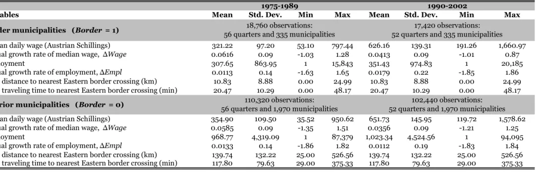
For our baseline results, we de…ne Border as comprising all municipalities whose geographic center is at most 25 road kilometers away from the nearest eastern border crossing, and “eastern” is de…ned as comprising all four formerly planned economies adjacent to Austria (Czech Republic, Hungary, Slovakia and Slovenia). A map of these municipalities is given in Figure 3.
In Table 3, we present descriptive statistics separately for border and interior municipali-ties. The table shows that border municipalities had relatively low wages and were compara-tively small in employment terms throughout the period covered by the data. Such di¤erences
in levels could be explained by a multitude of factors that it would be di¢ cult to control for comprehensively. The same is true for changes over time across all municipalities: why some municipalities on average grow faster than others could be due to a range of variables it again would be impossible to capture in its entirety. This is why we focus on di¤erences in changes pre- and post-1990 between border and interior regions. No major shock coincided with that timing and geographic reach other than the opening of the Eastern markets.22
Our baseline econometric estimates are shown in Table 4. Column 1 reports the coe¢ cient b from an estimation of the wage equation (1). The estimated coe¢ cient implies that over the 13 years subsequent to the fall of the Iron Curtain, nominal wages grew 0.27 percentage points faster annually in border regions than in interior regions, relative to their respective pre-1990 growth rates. This e¤ect is statistically signi…cant at the …ve-percent level. It suggests that improved market access after the opening of Eastern markets has boosted nominal wages in the most a¤ected Austrian municipalities. The corresponding estimate for employment growth, the coe¢ cient b from an estimation of equation (2), is given in column 2 of Table 4. We again …nd a positive impact. The treatment e¤ect of improved Eastern market access on the relative employment growth of border relative to interior regions is estimated as 0.86 percentage points, which is statistically signi…cant at the one-percent level. In cumulative terms, our benchmark parameter estimates imply that, thanks to the opening of the Central and Eastern European markets, Austrian border regions experienced an approximately 5 percent increase in nominal wages, and a 13 percent increase in employment, relative to regions in the Austrian interior.23
Our estimated coe¢ cients b and b suggest that trade liberalization has boosted wages as well as aggregate employment in Austrian border regions, but that the employment e¤ect was some three times larger than the e¤ect on wages (i.e. b = 0:8610:267 = 3:22). In this sense, employment was more responsive to changes in market access than nominal wages. The three tests shown in the bottom rows of Table 4 suggest that we can reject the hypothesis that b = 7, as implied by the theoretical model of Section 2, but not that b = 3, nor in fact that b = 1.
Columns 3 and 4 of Table 4 show corresponding estimates with the respective dependent
2 2One potentially confounding event was the eligibility of the Burgenland region for EU regional funds from
1995 onwards. We control for this in the robustness section, and …nd it to have no signi…cant e¤ect.
2 3The cumulative wage e¤ect is calculated as 100 (1 + w
I;F all+b)T (1 + wI;F all)T , where wI;F all
is the median post-1990 growth rate of interior-region wages (= 3:56%, see Table 3), and T is the number of post-1990 sample years (= 13). The cumulative employment e¤ect is calculated identically, mutatis mutandis.
variables de…ned as average annual changes over the entire pre- and post-1990 sample periods. This reduces the sample size but changes the results only trivially. The implied value ofb is very similar, with a point estimate of 3.05, and the hypothesis thatb = 7 is …rmly rejected.
Our baseline point estimates of are less than half as large as those implied by what we consider the most realistic calibration of the economic geography model of Section 2. If con…rmed, this would represent a considerable divergence between theory and empirics. Before concluding that the model implies too much interregional labor mobility (i.e. too high a value of ), we therefore need to ascertain that our estimated value ofb is a robust result.
5.2 Robustness
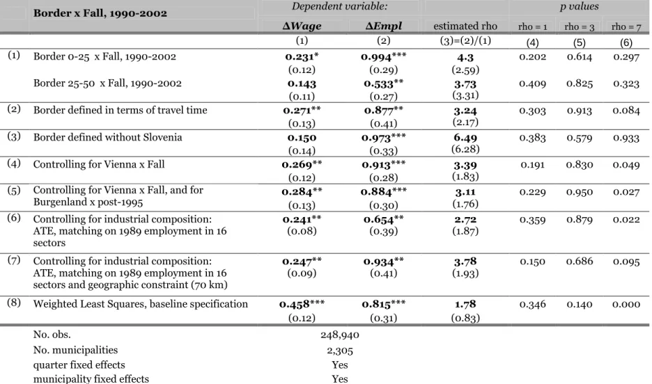
We begin by considering some alternative de…nitions of the treated region. In the …rst row of Table 5, we consider municipalities located between 25 and 50 kilometers from the eastern border as a second treatment group. Our baseline estimates for the municipalities in the 0-25 kilometer range are robust to this additional control: they retain their magnitudes and statis-tical signi…cance. Positive wage and employment e¤ects are also found for the municipalities in the 25-50 kilometer range. However, the e¤ects estimated for this outer band of border municipalities are only slightly more than half as large as those for the 25-kilometer border zone. Importantly, the estimated ratiob, at 3.73, is close to the baseline estimate obtained for the 0-25-kilometer treatment group. Experimentation with even wider border de…nitions never yielded any statistically signi…cant results. A corollary …nding of our study, therefore, is that the regionally di¤erentiated market access e¤ects were con…ned to a rather narrow set of locations in close proximity of the border.24
In a second robustness test, we use an alternative distance measure: estimated road trav-eling time to the nearest o¢ cial border crossing. This boils down to weighting roads by the speed at which they can be traveled. We report estimation results for a de…nition that at-tributes all municipalities located within 35 minutes from a border crossing to the treatment sample.25 The results, shown in the second row of Table 5, are essentially equivalent to those of our baseline regressions.
As another manipulation of our basic setup, we drop Slovenia from the sample of relevant
2 4
We provide further evidence of the steep spatial decay of the observed e¤ects in Section 5.3.
2 5The overlap between the Border sample under the 25-kilometer de…nition and under the 35-minute
de…ni-tion is large but not perfect. The 35-minute sample encompasses 276 municipalities, of which 248 also feature in the 25-kilometer sample.
eastern markets. This has two reasons. One is that Yugoslavia, even though a centrally planned economy, was not a member of the Soviet bloc and was economically more open prior to 1990 than Austria’s other eastern neighbor countries. The second reason is that the full potential of the Slovene market and those beyond it only emerged gradually over the 1990s, mainly as a result of the series of wars that accompanied the breakup of Yugoslavia.26 We report these results in the third row of Table 5. When dropping Slovenia as a relevant eastern market, we …nd weaker evidence of a wage response and stronger evidence of an employment response among the municipalities in the reduced-size treatment group. However, these coe¢ cients are very imprecisely measured, and we can reject none of the three hypotheses onb.
In a second set of robustness checks, we consider alternative de…nitions of the control group. One potentially confounding feature of our empirical setting is the existence of Vienna - by far the largest Austrian city. Vienna is located 64 kilometers, or 55 minutes, from the nearest eastern border (with Slovakia). It therefore is not included in our narrowly de…ned treatment groups. As it accounted for some 40 percent of Austrian employment in our data set overall, we nevertheless want to examine our baseline results against a speci…cation that controls speci…cally for the 23 municipalities that constitute the city of Vienna. As can be seen in row 4 of Table 5, controlling for Vienna barely a¤ects our baseline …ndings.
One might furthermore suspect some of our measured e¤ects to be due to the region of Burgenland. As shown in Figure 3, this region strongly overlaps with the set of municipalities de…ned as border regions with Hungary. Due to its relatively low per-capita income, Burgen-land was granted Objective 1 status subsequent to Austria’s accession to the European Union in 1995, making it eligible for generous regional subsidies. We therefore add a dummy variable that is equal to one for all observations that belong to Burgenland from 1995 onwards. These estimations are shown in the …fth row of Table 5. The inclusion of this control variable also has no signi…cant e¤ect on our coe¢ cient estimates of interest.27
We next estimate our baseline models in samples of municipalities that are matched on industry-level employment. Thereby, we can examine whether our results might be driven
2 6Figure 1 shows that Austrian trade with former Yugoslavia only took o¤ around 1995 and did not expand
to quite the same relative extent as trade with the three other Eastern neighbour countries.
2 7The coe¢ cients on the Burgenland controls themselves, which we do not show in Table 5, are never
statistically signi…cant. Hence, Objective 1 status appears to have had no discernible impact on aggregate employment and wage growth in Burgenland.
by the fact that border municipalities happened to be specialized in sectors that experienced particularly pronounced growth after 1990. Rows 6 and 7 of Table 5 show average treatment e¤ects of a matching estimator applied to di¤erences in growth rates between the post-1990 and the pre-1990 periods. We match municipalities on employment levels in 16 industries. In row 7 of Table 5, we furthermore restrict the matched control municipalities to lie no further than 70 kilometers from the treatment municipalities. Since we match by the size of industries in terms of employment (and not in terms of employment shares), our matching strategy also controls for di¤erences in the size of municipalities. Again we …nd statistically signi…cant treatment e¤ects on employment as well as on wages, and ratios of close to 3.
As a …nal check on our baseline results, we estimate speci…cations (1) and (2) using weighted least squares regression, taking sample-average municipal employment as weights, so as to reduce the weight of very small municipalities. As shown in row 8 of Table 5, our qualitative …ndings remain unchanged, but the magnitudes and statistical signi…cance of the relevant coe¢ cients increase. The wage e¤ect is now statistically signi…cant at the one-percent level as well, with the employment e¤ect estimated to be only 1.78 times as large as the wage e¤ect. Our baseline estimated values of the wage and employment e¤ect, however, remain within the 95-percent con…dence intervals also of these estimates.
For the eight speci…cations reported as robustness tests, we obtain estimated ratios of employment to wage adjustment, b, ranging from 1.78 to 6.49 (Table 5, column 3). The hypothesis tests shown in columns 4 to 6 of Table 5 allow us to reject the hypothesisb = 7, which is implied by what we consider the most plausible calibration of the theoretical model of Section 2, in six of our eight runs. The hypothesis b = 3, however, is never rejected. Hence, the data do appear to point to relatively less quantity adjustment than predicted by the theory.
One aspect that our data do not allow us to control for is individual worker characteristics. We therefore cannot distinguish wage increases that are due to skill upgrading from wage increases that are due to higher wage premia for identically skilled workers. Recent work by Frías, Kaplan and Verhoogen (2009) suggests that di¤erential industry-level trade-induced wage changes are explained almost entirely by wage premia, with no signi…cant explanatory power for skill upgrading. Their result is based on Mexican data, where skill upgrading would appear a more likely adjustment channel than in Austria. Based on this evidence, skill
upgrading does not appear as a likely unobserved confound biasing our results.
5.3 Non-Parametric Illustrations: Space and Time
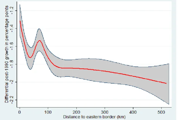
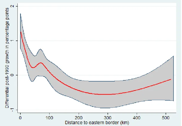
So far, we have imposed a dichotomy between treatment (Border = 1) and control (Border = 0) municipalities. We now relax this by estimating speci…cations (3) and (4) and plotting the estimated post-1990 growth di¤erential of each municipality against that municipality’s distance from the eastern border. The plot for wages is given in Figure 4 and that for employment is given in Figure 6. Circles in these graphs are scaled according to municipal employment.
The raw scatter plots do not look particularly informative. Nonetheless, a statistically signi…cant relationship exists. This becomes clear in the corresponding natural spline regres-sions shown in Figures 5 and 7 respectively.28 The plots show that there is a statistically signi…cantly positive e¤ect on both wages and employment for municipalities that are located close to Austria’s eastern border, whereas there is none for municipalities beyond about 50 kilometers from the border, with Vienna representing an evident outlier.
This representation con…rms that the di¤erential e¤ect of post-1990 market opening was con…ned to a relatively narrow band of Austrian municipalities located close to the border. Our analysis corroborates the relatively sharp distance decay of intra-national market-access and agglomeration e¤ects found elsewhere (see, e.g., Rosenthal and Strange, 2003).
Although the theory does not feature explicit dynamics, we consider it interesting to inves-tigate the time pro…le of our estimated treatment e¤ects. We can describe the disaggregate time pro…le within that period by estimating speci…cations (5) and (6). These regressions provide us with annual estimates of di¤erential wage changes (bt) and employment changes
(bt) in border regions for each year post-1990. The results are shown in Figures 8 and 9. In most sample years, border-region wage and employment growth rates did not diverge sta-tistically signi…cantly from those in interior regions. We do, however, observe two periods over which signi…cant treatment e¤ects are in evidence: in 1995-1997, border-region nomi-nal wages exhibit signi…cantly positive di¤erential growth, and in 1997-2000 a corresponding spike is observed for border-region employment growth. Our results thus suggest that wages
2 8
The smoothed lines are obtained by creating variables containing a cubic spline with seven nodes of the variable on the horizontal axis (distance to the eastern border), and by plotting the …tted values obtained from an employment-weighted regression of the dependent variable (post-1990 growth wage/employment growth) on the spline variables.
adjusted earlier than employment, which is consistent with the view that wages are quicker to react to changed market conditions (at least in upward direction) than employment levels. Note, however, that both responses occur with a lag of some …ve years after the fall of the Iron Curtain. This is likely due not only to sluggish market responses but also to gradualism in the reduction of trade barriers and to persistence of political risk (with fears of a political backlash in Eastern Europe persisting well into the 1990s).
6
Revisiting the Model
6.1 Allowing for Preference Heterogeneity
We …nd the magnitude of employment adjustment to equal around three times that of wage adjustment in our data - considerably lower than the ratio predicted by the most plausible calibration of the theoretical model of Section 2. Table 1 shows that, for the model to predict a ratio of 3, we would need a housing share (1 ) of between 0.4 and 0.5. This is too high to be realistic. We therefore conclude that the Helpman (1998) variant of the three-region economic geography model predicts too much employment adjustment and too little wage adjustment. For a better match between the theory and our empirical result, a stronger dispersion force is needed than that represented by housing alone.
We therefore consider a simple extension to the model by allowing for a plausible (though not the only conceivable) additional dispersion force: randomly distributed idiosyncratic lo-cational preferences, following Tabuchi and Thisse (2002) and Murata (2003). Details of the model are again given in the Appendix. Preference heterogeneity is modelled through the parameter 2 (0; 1). When = 0, individuals have identical preferences and choose their region of residence solely according to the indirect utility derived from their consumption of M and H. This is the preference structure of the model we considered in Section 2. As increases, idiosyncratic locational preferences become more important, and in the extreme case of ! 1 they alone determine workers’location choices.
There is neither empirical nor theoretical guidance as to what value to assign to . We will, however, be able to gauge the plausibility of values of indirectly. The presence of heterogeneity gives rise to regional real-wage di¤erences that are not eliminated by migration precisely because, with heterogeneity, there will be some workers who prefer not to migrate
despite thereby foregoing an increase in the real wage. We can thus assess values of by looking at the implied share of workers that do not move despite a given regional di¤erence in real wages. For a plausibility check, we can draw on some related empirical evidence, based on the mobility of unemployed workers (see Shields and Shields, 1989, for an early survey). Faini, Galli, Gennari and Rossi (1997) found that the percentage of Italian unemployed re-fusing to move out of their town of residence if a job were available elsewhere ranges from 21 percent (Northern male university graduates) to 61 percent (Southern low-education females). Fidrmuc (2005) reported survey evidence according to which 34 percent of EU15 unemployed and 25 percent of Czech unemployed stated in 2002 that they would not move under any circumstances even if a job became available elsewhere. These studies point towards consider-able locational inertia even within countries, supporting the relevance of incorporating factors other than wage di¤erentials among the determinants of labor mobility in models of economic geography.
We allow to take any non-negative value, and search for the value of that yields an equilibrium of 3.29 For each of these simulations we report the implied interregional real-wage di¤erence and the implied population share of non-movers at that real-real-wage di¤erence. The combination of these numbers allows us to gauge the plausibility of the implied value of
.30
The corresponding results are reported in Table 6. Each cell of that table shows the implied percentage real-wage di¤erential between regions within country A and, in brackets, the implied share of country A’s population that prefers not to migrate at the prevailing real-wage di¤erential. Table 6 shows that allowing for heterogenous locational preferences allows us to align the model’s predictions with our estimated . We consider eight parameter combinations for and (1 ), taking what we deem the most plausible values of these parameters. In all eight cases, a relatively small amount of preference heterogeneity su¢ ces to produce a predicted value of = 3. The necessary degree of preference heterogeneity when = 4 and (1 ) = 0:25, for instance, is such that 16 percent of the population would not
2 9
We stop the search loop at the …rst iteration that implies a value of between 2.9 and 3.1.
3 0If, for instance, in order to obtain a of 3, had to be such that the real-wage di¤erence between regions
were 200 percent and the immobile population share were 95 percent, then, given the low plausibility of such a con…guration, we would conclude that taste heterogeneity is not a useful modeling feature for matching the theory to the facts. Conversely, to the extent that equilibrium real-wage di¤erentials and immobile population shares look plausible, heterogeneity in locational tastes can be considered an empirically relevant addition to the model.
move even if the real wage were 28 percent higher in the other region. In light of the available European evidence on the issue, this does not appear to be an excessive dose of assumed intrinsic insensitivity to regional wage di¤erentials.
6.2 Discussion
Our simulations suggest that the baseline economic geography model with housing as the sole dispersion force implies more labor mobility than our empirical estimates, and there-fore overpredicts the importance of the employment adjustment channel relative to the wage adjustment channel. If we extend the baseline model by including a moderate amount of lo-cational taste heterogeneity, we can easily reconcile the theoretical model with the empirical estimates.
On the face of it, our central result therefore stands in contrast to the …ndings of Hanson (2005) and Redding and Sturm (2008), who both concluded that the calibrated Helpman (1998) model …t their empirical estimates well.
For parameter values in the same range as those used in our paper, Redding and Sturm (2008) found that the Helpman model can replicate the growth di¤erential of small and large cities subsequent to the loss of access to eastern markets following the division of Germany. Their analysis concentrated on adjustment via factor quantities, measured by population, as wage data are not available for the long time period covered by their study. Our results suggest that their conclusions might have been di¤erent had they been able to consider wage data. To see this, consider for instance the ten combinations of and (1 ) that Redding and Sturm (2008, Table 3) have identi…ed as o¤ering the best match between the model and their empirical estimates. In each case, we can apply these parameters to the unamended (Helpman) variant of the three-region model and indeed …nd levels of trade integration, BR, for which
the model precisely matches the estimated coe¢ cient of the baseline employment regression, b = 0:86 (see Table 4). The implied values of across these ten calibrations range from 3.2 to 11.8. Only two calibrations yield s below 4, and they both imply rather large housing shares (of 42 and 48 percent respectively). The parameter con…gurations in the plausible range, i.e. with housing shares below 0.3, all yield s in excess of 6. Hence, information on wage e¤ects does appear to be important for a full evaluation of the congruence between the theory and the data.
The analysis by Hanson (2005) concentrated on adjustment via factor prices, by estimating a structural wage equation of the Helpman model on US county data. His estimations imply plausible parameter values, with predicted housing shares if anything on the low side.31 A comparison of his results to ours thus suggests that obstacles to labor mobility, even at a small spatial scale, are higher in Europe than in the United States. The logical upshot is that, while a geography model with immobile housing and homogeneous locational tastes o¤ers a good …t with observed spatial adjustment the North American context, an additional dispersion force, such as heterogeneous tastes, ought to be considered in a European setting.
This result has implications for policy. It is an additional piece of evidence pointing to relatively lower labor mobility in Europe than in North America, even within countries. Hence, trade and other shocks with regionally asymmetric e¤ects can bring about greater intra-national spatial wage inequality in Europe than in North America. However, if trade liberalization bene…ts previously low-wage regions as in the case of eastern Austria, then it can act to reduce spatial inequality.
7
Conclusions
We have used the opening of Central and Eastern European markets after the fall of the Iron Curtain as a natural experiment of the e¤ects of trade liberalization on regional wages and employment. Identi…cation is achieved by comparing di¤erential pre- and post-liberalization growth rates of wages and employment between, on the one hand, Austrian regions located close to the border to the formerly closed and centrally-planned eastern economies and, on the other hand, Austrian regions further away from the border.
We …nd that trade liberalization has had statistically signi…cant di¤erential e¤ects on both nominal wages and employment of a rather narrow band of border regions. Most of the observed impact was con…ned to locations within 25 kilometers of the border, and no statistically signi…cant e¤ects are found beyond a distance of 50 kilometers.
The estimated e¤ect on employment exceeds the estimated e¤ect on nominal wages by a factor of around three. Over the entire post-Iron Curtain period, locations within 25 kilome-ters of the border are estimated to have experienced a 5 percent increase in nominal wages
3 1
Hanson’s (2005) mean parameter estimates across the four reported variants of the instrumented regressions
and a 13 percent increase in employment, relative to regions in the Austrian interior.
Wages are found to have reacted earlier than employment, consistent with the view that wages rise more quickly than employment levels in response to increases in regional demand. We then calibrated a standard economic geography model featuring immobile housing and compared the implied predictions to our estimation results. This comparison suggests that the model somewhat overpredicts the relative magnitude of employment adjustment and thereby implies too much mobility. When augmented by heterogeneous locational preferences, which adds an impediment to employment adjustment, the model is easily able to replicate the estimated ratio of employment and wage adjustment.
References
[1] Ades, Alberto F. and Glaeser, Edward L. (1995) Trade and Circuses: Explaining Urban Giants. Quarterly Journal of Economics, 110: 195-227.
[2] Baier, Scott L. and Bergstrand, Je¤rey H. (2001) The Growth of World Trade: Tari¤s, Transport Costs, and Income Similarity. Journal of International Economics, 53: 1-27. [3] Baldwin, Richard E.; Forslid, Rikard; Martin, Philippe; Ottaviano, Gianmarco I.P. and
Robert-Nicoud, Frédéric (2003) Public Policies and Economic Geography. Princeton Uni-versity Press.
[4] Broda, Christian and Weinstein, David E. (2006) Globalization and the Gains from Variety. Quarterly Journal of Economics, 121: 541-585.
[5] Bernard, Andrew B.; Eaton, Jonathan; Jensen, J. Bradford and Kortum, Samuel (2003) Plants and Productivity in International Trade. American Economic Review, 93: 662-675. [6] Bertrand, Marianne; Du‡o, Esther and Mullainathan, Sendhil (2004) How Much Should We Trust Di¤erences-in-Di¤erences Estimates? Quarterly Journal of Economics, 119: 249-275.
[7] Brülhart, Marius; Crozet, Matthieu and Koenig, Pamela (2004) Enlargement and the EU Periphery: The Impact of Changing Market Potential. World Economy, 27(6): 853-875. [8] Buettner, Thiess and Rincke, Johannes (2007) Labor Market E¤ects of Economic Inte-gration: The Impact of Re-Uni…cation in German Border Regions. German Economic Review, 8: 536-560.
[9] Chiquiar, Daniel (2008) Globalization, Regional Wage Di¤erentials and the Stolper-Samuelson Theorem: Evidence from Mexico. Journal of International Economics, 74: 70-93.
[10] Combes, Pierre-Philippe; Lafourcade, Miren and Mayer, Thierry (2005) The Trade-Creating E¤ects of Business and Social Networks: Evidence from France. Journal of International Economics, 66: 1-29.
[11] Davis, Donald R. and Weinstein, David E. (1999) Economic Geography and Regional Production Structure: An Empirical Investigation. European Economic Review, 43: 379-407.
[12] Davis, Morris A. and Ortalo-Magné, François (2011) Household Expenditures, Wages, Rents. Review of Economic Dynamics, 14: 248-261.
[13] Dickens, William T.; Goette, Lorenz; Groshen, Erica L.; Holden, Steinar; Messina, Julian; Schweitzer, Mark E.; Turunen, Jarkko and Ward, Melanie E. (2007) How Wages Change: Micro Evidence from the International Wage Flexibility Project. Journal of Economic Perspectives, 21: 195-214.
[14] Faber, Benjamin (2009) Integration and the Periphery: The Unintended E¤ects of New Highways in a Developing Country. Mimeo, London School of Economics.
[15] Faini, Riccardo; Galli, Gianpaolo; Gennari, Pietro and Rossi, Fulvio (1997) An Empir-ical Puzzle: Falling Migration and Growing Unemployment Di¤erentials among Italian Regions. European Economic Review, 41: 571-579.
[16] Fidrmuc, Jan (2005) Labor Mobility During Transition: Evidence from the Czech Re-public, CEPR Discussion Paper #5069.
[17] Frías, Judith A.; Kaplan, David S. and Verhoogen, Eric A. (2009) Exports and Wage Premia: Evidence from Mexican Employer-Employee Data. Mimeo, Columbia University. [18] Hanson, Gordon H. (1997) Increasing Returns, Trade and the Regional Structure of
Wages. Economic Journal, 107: 113-133.
[19] Hanson, Gordon H. (1998) Regional Adjustment to Trade Liberalization. Regional Sci-ence and Urban Economics, 28: 419-444.
[20] Hanson, Gordon H. (2005) Market Potential, Increasing Returns and Geographic Con-centration. Journal of International Economics, 67: 1-24.
[21] Head, Keith and Mayer, Thierry (2004) The Empirics of Agglomeration and Trade. In: Henderson, J.V. and Thisse, J.F. (eds) Handbook of Regional and Urban Economics, Elsevier.
[22] Head, Keith, and Mayer, Thierry (2006) Regional Wage and Employment Responses to Market Potential in the EU. Regional Science and Urban Economics, 36: 573–594. [23] Helble, Matthias (2007) Border E¤ect Estimates for France and Germany Combining
International Trade and Intranational Transport Flows. Review of World Economics, 143: 433-463.
[24] Helpman, Elhanan (1998) The Size of Regions. In: Pines, D., Sadka, E. and Zilcha, I. (eds.) Topics in Public Economics: Theoretical and Applied Analysis, Cambridge Uni-versity Press, 33-54.
[25] Henderson, J. Vernon (2003) The Urbanization Process and Economic Growth: The So-What Question. Journal of Economic Growth, 8: 47-71.
[26] Hillberry, Russell and Hummels, David (2003) Intranational Home Bias: Some Explana-tions. Review of Economics and Statistics, 85: 1089-1092.
[27] Hillberry, Russell and Hummels, David (2008) Trade Responses to Geographic Frictions: A Decomposition Using Micro-Data. European Economic Review, 52: 527-550.
[28] Krugman, Paul (1991) Increasing Returns and Economic Geography. Journal of Political Economy, 99: 483-499.
[29] Miyao, Takahiro (1978) A Probabilistic Model of Location Choice with Neighborhood E¤ects. Journal of Economic Theory, 19: 347–358.
[30] Murata, Yasusada (2003) Product Diversity, Taste Heterogeneity, and Geographic Dis-tribution of Economic Activities: Market vs. Non-Market Interactions. Journal of Urban Economics, 53: 126-144.
[31] OECD (2001) Migration Policies and EU Enlargement: The Case of Central and Eastern Europe. OECD, Paris.
[32] Redding, Stephen and Sturm, Daniel (2008) The Costs of Remoteness: Evidence from German Division and Reuni…cation. American Economic Review, 98: 1766-1797.
[33] Redding, Stephen and Venables, Anthony J. (2004) Economic Geography and Interna-tional Inequality. Journal of InternaInterna-tional Economics, 62: 53-82.
[34] Rosenthal, Stuart S. and William C. Strange (2003) Geography, Industrial Organization, and Agglomeration. Review of Economics and Statistics, 85: 377-393.
[35] Sanguinetti, Pablo and Volpe Martincus, Christian (2009) Tari¤s and Manufacturing Location in Argentina. Regional Science and Urban Economics, 39: 155-167.
[36] Shields, Gail M. and Shields, Michael P. (1989) The Emergence of Migration Theory and a Suggested New Direction. Journal of Economic Surveys, 3: 277-304.
[37] Tabuchi, Takatoshi and Thisse, Jacques-François (2002) Taste Heterogeneity, Labor Mo-bility and Economic Geography. Journal of Development Economics, 69: 155-177. [38] Zweimüller, Josef; Winter-Ebmer, Rudolf; Lalive, Rafael; Kuhn, Andreas; Wuellrich,
Jean-Philippe; Ruf, Oliver and Büchi, Simon (2009) Austrian Social Security Database. Working Paper #0903, Austrian Center for Labor Economics and the Welfare State, University of Linz.
A
Appendix: Theoretical Model
We use multi-region versions of a model that combines features of Krugman (1991), Helpman (1998), Tabuchi and Thisse (2002) and Murata (2003).32
A.1 Demand
The world economy consists of regions and is populated by a given mass of individuals, L, indexed by k. We divide the set of all regions into two subsets, which we call “countries”, A(ustria) and R(est of the world). For notational convenience, we assume that regions 1 to belong to country A, while the remaining regions belong to country R. Labor is mobile within countries but immobile between countries.
Each individual is endowed with one unit of labor, which is the only factor of production. Individuals derive utility from the consumption of goods as well as, potentially, from an exogenous and idiosyncratic preference parameter associated with individual regions.
The component of utility that is associated with consumption is modelled as a Cobb-Douglas combination of a CES (Dixit-Stiglitz) aggregate of varieties of a tradeable good, M , and consumption of a non-tradeable resource, H:
U = CM CH 1 ; 0 < < 1:
Since H is a non-tradeable and exogenously given local resource, we refer to it as “housing”, following Helpman (1998).
Trade among regions incurs costs of the conventional “iceberg” type, whereby for each unit of a variety sent from location i to location j only a fraction ij 2 (0; 1) arrives at its
destination. Trade within regions is free, ii= 1; 8 i; and bilateral trade costs are symmetric, ij = ji 8 i; j. Utility maximization under the budget constraint gives individual demand


![Table 6: Extended Model: Implied Immobility for ρ ≈ 3 = 3 = 4 = 5 = 6 25 29 30 31 (1- ) = 0.20 [19] [22] [23] [25] 24 28 31 32 (1- ) = 0.25 [14] [16] [17] [18] 20 25 27 29 (1- ) = 0.30 [10] [12] [12] [12]](https://thumb-eu.123doks.com/thumbv2/123doknet/14569184.539354/42.892.77.488.109.269/table-extended-model-implied-immobility-ρ.webp)
