GJI
Seismology
Thermochemical interpretation of one-dimensional seismic reference
models for the upper mantle: evidence for bias due to heterogeneity
Laura Cobden,
1Saskia Goes,
1Fabio Cammarano
2and James A. D. Connolly
31Department of Earth Science and Engineering, Imperial College London, London SW7 2AZ, UK. E-mail: [email protected] 2Berkeley Seismological Laboratory, UC Berkeley, CA, USA
3Institute of Mineralogy and Petrography, ETH Zurich, Zurich, Switzerland
Accepted 2008 June 27. Received 2008 June 27; in original form 2007 December 20
S U M M A R Y
A 1-D reference model for the mantle that is physically meaningful would be invaluable both in geodynamic modelling and for an accurate interpretation of 3-D seismic tomography. However, previous studies have shown that it is difficult to reconcile the simplest possible 1-D physical model—1300◦C adiabatic pyrolite—with seismic observations. We therefore generate a set of alternative 1-D thermal and chemical mantle models, down to 900 km depth, and compare their properties with seismic data. We use several different body and surface wave data sets that provide complementary constraints on mantle structure. To assess the agreement between our models and seismic data, we take into account the large uncertainties in both the elastic/anelastic parameters of the constituent minerals, and the thermodynamic procedures for calculating seismic velocities. These uncertainties translate into substantial differences in seismic structure. However, in spite of such differences, subtle trends remain. We find that models which attain (1) higher velocity gradients between 250 and 350 km; (2) higher velocity gradients in the lower transition zone; and (3) higher average velocities immediately beneath the 660-discontinuity, than 1300◦C adiabatic pyrolite—either via a temporary shift to lower temperatures, and/or a change to a seismically faster chemical composition—provide a significantly better fit to the seismic data than adiabatic pyrolite. This is compatible with recent thermochemical dynamic models by Tackley et al. in which average thermal structure is smooth and monotonous, but average chemical structure deviates substantially from pyrolite above, in, and below the transition zone. Our results suggest that 1-D seismic reference models are being systematically biased by a complex 3-D chemical structure. This bias should be taken into account when attempting quantitative interpretation of seismic anomalies, since those very anomalies contribute to the 1-D average signal.
Key words: Mantle processes; Composition of the mantle; Equations of state; Phase
transi-tions; Body waves; Seismic tomography.
I N T R O D U C T I O N
Over 90 per cent of the global seismic data available today can be represented by one-dimensional, radially symmetric wave speed models. Such models, e.g., PREM (e.g. Dziewonski & Anderson 1981) and AK135 (Kennett et al. 1995), form the basis for 3-D seismic tomography, in which lateral variations in wave speed are measured as a percentage difference, or anomaly, relative to the cho-sen 1-D reference model (e.g. Grand et al. 1997; Su & Dziewonski 1997; Kennett et al. 1998).
However, seismic models themselves do not tell us about the underlying dynamic behaviour of the mantle—for this we need to know a range of physical variables, most importantly chemical composition and temperature, and we cannot elucidate a unique
combination of these variables from any particular seismic model. Given the similarity between the different 1-D seismic reference models, and the smallness of the deviations of 3-D structure away from these references, one might expect that the reference models represent the average 1-D physical structure of the mantle. If we were able to define such a physical structure, it would provide an important constraint in geodynamic modelling, and allow a better understanding of mantle dynamics. Not only that, but as technolog-ical advances allow increasingly higher resolution of 3-D structures in seismic tomography, there is a greater impetus to interpret these structures quantitatively in terms of dynamically relevant parame-ters (Trampert & Van der Hilst 2005). Such interpretations are only possible if we can relate a tomographic reference seismic model to an absolute thermochemical structure.
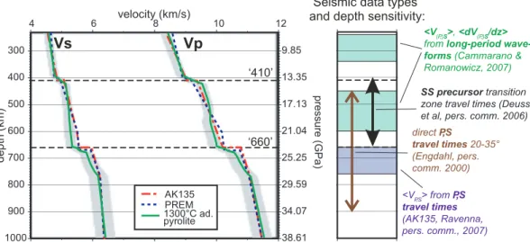
Figure 1. Comparison of 1300◦C adiabatic pyrolite with the seismic references AK135 and PREM (left-hand side), together with summary of seismic data types used in this study and their depth sensitivities (right-hand side). Grey bands indicate uncertainty on adiabatic pyrolite model.
Whilst it is not possible to convert a seismic structure directly into a unique physical structure, any plausible physical model for the mantle must have seismic properties which are in agreement with global observations. In line with this requirement, Cammarano et al. (2005a,b) calculated the seismic properties of a simple 1-D physical mantle model and compared them with seismic data (tele-seismic travel times and normal mode frequencies). Their model was designed with the assumption of whole mantle convection, combined with petrological constraints, resulting in a mantle with constant chemical composition—pyrolite—and a temperature pro-file following an abiabat with a potential temperature of 1300◦C. Previously, several authors have inferred that such a model is suf-ficient to explain fully the 1-D seismic reference models PREM or AK135 (e.g. Weidner 1985; Ita & Stixrude 1992; Jackson & Rigden 1998).
However, Cammarano et al. (2005a,b) found that, within the uncertainty bounds of the mineral physics data that they used, the seismic behaviour of their 1300◦C-adiabatic-pyrolite (13AP) model did not fit global observations well. This misfit is illustrated in Fig. 1: Relative to reference model AK135 (which does fit the seis-mic data), 1300◦C adiabatic pyrolite has a lower velocity gradient in the transition zone, and a smaller velocity jump at the 660-discontinuity. It has lower average velocities and higher velocity gradients in the uppermost lower mantle.
There are two possible causes for the discrepancy between the models of Cammarano et al. (2005a,b) and seismic data:
1. Underestimation of the uncertainties in the mineral physics data and equations of state used to model the mantle.
2. Their assumed mantle thermochemical structure is unrepre-sentative of the real mantle.
In this paper, we address the first of these possibilities by employ-ing several different techniques to compute seismic velocities. We do this for each of our mantle models, as far as the current mineral elasticity data permit. We also create sets of thousands of models based on the 1300◦C adiabatic pyrolite, in which the mineral elastic and anelastic parameters are varied randomly, within generous but pre-defined uncertainty bounds, from model to model (Cammarano et al. 2005a). By performing these two tests, we gain a sense for the extent to which mineral physics uncertainties influence the seismic
misfit of our models, which in turn allows us to distinguish if and when particular seismic behaviour is due to alternative underlying thermochemical structure.
We explore the second possibility by calculating the seismic prop-erties of a range of alternative 1-D thermal and chemical models to 1300◦C adiabatic pyrolite, up to 900 km depth. We particu-larly focus on the seismic behaviour in and around the transition zone (∼250–750 km depth), where significant discrepancy between models and observations was noted by Cammarano et al. (2005a). We study the fit of our models to travel time data for both direct P and S phases and SS-precursors. We also compute average ve-locities and velocity gradients over specific depth intervals, and compare them with values inferred from long period waveform inversions.
C O M P U T AT I O N O F S E I S M I C
V E L O C I T I E S A N D U N C E RT A I N T I E S
Generation of seismic velocities for a given thermochemical struc-ture requires the following steps:
(1) A bulk chemical composition is defined. In this paper, com-positions are expressed in terms of the relative proportions of five oxide endmembers: CaO, FeO, MgO, Al2O3and SiO2 (CFMAS), which make up more than 98 per cent of MORB-source mantle (pyrolite).
(2) A temperature–pressure (T –P) structure is defined, typically an adiabat.
(3) A phase diagram for the chosen bulk chemical composition is used to infer the relative proportions of each mineral at each point in the temperature–pressure structure.
(4) Using an equation of state (EoS), the elastic parameters for each mineral are extrapolated to high temperatures and pressures so that they are defined at each point in the T –P model.
(5) Anharmonic seismic velocities for each mineral at each T – P point are computed using the values of the elastic parameters inferred in (4). The overall seismic velocity at each T –P point is given by the weighted average of the velocities of the constituent minerals.
This calculation involves many uncertainties. For the upper man-tle and transition zone, the main sources of uncertainty are, in decreasing order of importance: uncertainties in the elastic and anelastic mineral parameters; the extrapolation of mineral elastici-ties to high pressures and temperatures; mineral phase relations at mid-mantle pressures; and calculation of mantle adiabats.
We consider the effect of (1) uncertainties in the calculation pro-cedure (i.e. equation of state, phase diagram, and the calculation of adiabats), and (2) uncertainties in the mineral parameters, sepa-rately. These are discussed in more detail below. In our diagrams, we then summarize the seismic manifestation of these two types of uncertainties with two contours. Appendix B shows and discusses the distributions behind the contours.
(1) Uncertainties in calculation procedure (EoS and phase diagram)
To evaluate these uncertainties we use two different methods to calculate velocities, with some variations in the level of approxima-tion used in them. The methods differ in steps (1–2), (3) and (4) as outlined above. Steps (5) and (6) are the same. These methods are explained fully in Appendix A. To summarize briefly:
The first method uses a third-order Birch-Murnagan EoS with a Gr¨uneisen correction for temperature. We will refer to this as 3E-Grun in the rest of the paper. This was the method used by Cammarano et al. (2005a,b) and is the most common EoS fit to experimental mineral data. We test a few variations on it—an update of the pyrolite phase diagram, an updated set of adiabats, and a non-linear rather than linear Gr¨uneisen tem-perature correction, compared to the original approach used by Cammarano et al. (2005a,b). Our preferred version, shown on all diagrams and labelled as 3E-Grun, includes all these up-dates (Method 3E-Grun-4 in Appendices A and B). With this method we also test mineral parameter uncertainties (see (2) below).
The second method is a third-order finite strain EoS with a Mie-Gr¨uneisen thermal pressure correction for temperature, which is coupled to the calculation of phase relations (after Stixrude & Lithgow-Bertelloni 2005a)—solved using the code Perple_X (Connolly 1990; Connolly 2005). This method—hereafter referred to as 3E-Mie—is the most ‘self-consistent’ approach, firstly because the same mineral physics data are used in all stages of the calcula-tion, from defining the mineral phase relations to computing seismic velocities. Secondly, the specific mineral parameter values chosen (Stixrude & Lithgow-Bertelloni 2005a) are derived from a large-scale global inversion of experimental and first-principles theoreti-cal data, rather than being taken directly from many different, inde-pendent raw data sets. However, the Stixrude & Lithgow-Bertelloni (2005a) database only provides a single value for each mineral pa-rameter, and a consequence of having obtained the parameters by inversion is that they are partially correlated. This hampers an evalu-ation of mineral uncertainties by assignment of uncorrelated uncer-tainties to individual parameters. We can do some evaluation of un-certainties using a newer database (Stixrude & Lithgow-Bertelloni 2007), which includes single parameter uncertainties (Appendix B). However, due to the different EoS used, it remains problematic to assert how ‘average’ or ‘extreme’ the data set may be relative to the extensive literature data compilation used in 3E-Grun. Except in Appendix B, all figures show 3E-Mie results calculated with the 2005 database.
(2) Uncertainties in mineral elastic (anharmonic) and anelastic parameters
Elastic parameter uncertainty
We generate 10 000 mantle models based on 1300◦C adiabatic pyrolite whose elastic parameters vary randomly within pre-defined uncertainty bounds (Cammarano et al. 2003), using a Monte Carlo procedure. These models are computed with the 3E-Grun method (3E-Grun-4 in Appendix A).
Random values are allocated to seven parameters: bulk modu-lus K; shear modumodu-lus G; their temperature and pressure derivatives ∂ K /∂T , ∂G/∂T , ∂ K /∂ P, ∂G/∂ P; and thermal expansion coef-ficientα, for the nine major mantle minerals (olivine, wadsleyite, ringwoodite, clinopyroxene, orthopyroxene and garnet in the upper mantle; Mg-perovskite, Ca-perovskite and periclase in the lower mantle). To enhance computational efficiency, random values are only assigned to the magnesian end-members of each of these min-erals, since these dominate volumetrically, although Ca, Fe and Al end-members are of course included in all phase equilibria and velocity calculations, as are minor minerals not given in the nine listed above. The seismic manifestation of uncertainties in these minor components is insignificant in comparison to the effect of uncertainties in the major components calculated here.
The uncertainty bounds on those elastic parameters which do vary are based on a compilation of experimental data (Cam-marano et al. 2003). They are sufficiently generous that they en-capsulate the entire range of experimentally determined values obtained for that parameter (up to 2003). Each model has the same anelasticity structure, model Q5 (Cammarano et al. 2003). Our analysis indicates that 10 000 models is a sufficiently large sample to assess the effect of uncertainties in elastic parameters on seismic behaviour, in spite of the large solution space of the elastic parameters (see Appendix B, Section ‘Mineral parameter uncertainties’).
Combined elastic and anelastic parameter uncertainties
Anelasticity causes attenuation and dispersion of seismic waves. It significantly influences seismic velocities in the mantle (Karato 1993), especially at high temperatures relative to the melting tem-perature, due to viscoelastic relaxation, and must be incorporated into our models (Appendix A, step 6). Reference global anelasticity models such as QL6 (Durek & Ekstrom 1996) and PAR3C (Okal & Jo 1990) have been proposed on the basis of seismic data. How-ever, the precise form of the Earth’s average anelasticity structure is uncertain.
We therefore use a set of anelasticity models (models Q1–Q6 of Cammarano et al. (2003)) which span both within and well outside the range covered by the reference models QL6 and PAR3C, in order to determine the maximum possible effect of anelasticity on seismic properties. We take the same 10 000 models used to evaluate the elastic parameter effects, but now assign randomly to each model one of the six structures Q1–Q6. This allows us to understand the combined effect of elastic and anelasticity parameters on seismic velocities and travel times.
Appendix B illustrates that at the temperatures and depths we consider here (250–800 km), the effect of elastic parameter un-certainties overlaps that of the combined anelastic plus elastic pa-rameter uncertainties, and as such only the 90 per cent confidence contour of the latter is shown in the subsequent figures.
S E I S M I C D AT A U S E D F O R C O M PA R I S O N
We test our models against three different sets of global seismic data: direct P- and S-wave arrival times, SS-precursor arrival times, and long-period waveforms. The range of seismic data types yields com-plementary, and hence more comprehensive, constraints on mantle structure. The actual parameters of our models that we test against the data comprise a mixture of (1) seismic travel times, for which we are comparing model values directly with the (global average of) seismic data itself; and (2) seismic velocities and velocity gradi-ents, in which the original seismic data must be passed through an inversion procedure before they can be compared with our models. Travel times have the advantage that the seismic properties against which the models are tested have not been biased by any inversion procedure, whilst average velocities and velocity gradi-ents have the advantage that a large number of models can be tested speedily against properties that have been tightly constrained by a huge seismic database. For although there is considerable uncer-tainty in the inverted velocity value at a single depth, average veloc-ities and gradients over wider depth intervals are often extremely tightly constrained.
1. Direct P- and S- arrival times
Seismic travel times through our velocity models are calculated using a simple ray-tracing algorithm (Crotwell et al. 1999). We can distinguish structural changes with depth by studying all rays with turning points inside the depth interval of interest. For this reason, we study direct P arrivals in the angular distance range 18.75◦–35.25◦, and direct S arrivals in the range 19.75◦–35.25◦, corresponding to rays with turning points in the transition zone and uppermost lower mantle. At shorter distances, there is an in-terference with crustal phases. We compare the arrival times of our models to data from the ISC catalogue up to 2000 (Engdahl et al. 1998; Engdahl et al. 2000, personal communication).
When computing travel times, we do not use our own calculated velocities for the lithosphere, given the high lateral variability of the crust and lithosphere in the Earth. Instead we place the AK135 crustal wave-speed structure in the top 35 km of each of our mod-els, and interpolate velocities between 35 km (AK135) and 80 km (our calculations) until they merge with our calculated wave-speed structure at 80 km. The arrival times we use in our study are only influenced by the average structure above the transition zone, and any variations in seismic behaviour due to crustal properties results in an almost-constant shift in all the arrival times. Therefore in our results, we illustrate the likely magnitude of such a shift in travel times by plotting the change in travel time due to using a PREM crust rather than an AK135 crust.
2. SS-precursor travel times
SS-precursors are weak S-wave arrivals which have reflected once off the underside of a mantle discontinuity before arriving at the Earth’s surface, and they arrive slightly earlier than their correspond-ing SS-arrival. They can be observed by stackcorrespond-ing many long-period global seismograms (Shearer 1991; Shearer 2000 and references therein). The term SdS is used to denote a precursor phase which has reflected off a discontinuity at depth ‘d’. In contrast to direct arrivals, SS-precursors can be manipulated to give a travel time through the transition zone exclusively. This is done by subtracting the arrival time of S660S from S410S, giving a travel time that is not
obscured by any structure above the transition zone. The one-way S travel time through the transition zone is approximately equal to (tS410S− tS660S)/2.
We use a stack of 7018 seismograms from the IRIS/IDA/USGS network, collected between 1980 and 1998, to obtain global aver-age values for the arrival times of S660S and S410S at an epicentral distance of 130◦(Deuss & Woodhouse 2001; Deuss, 2006, personal communication). A bootstrap resampling algorithm (Efron & Tib-shirani 1991) provides an estimate of the uncertainty on the S660S and S410S arrival times. We calculate from these data the global average one-way S travel time through the transition zone, with un-certainty bounds. This can then be compared with 1-way S travel times for our models which are calculated using the ray-tracing algorithm of Crotwell et al. (1999).
3. Average velocities and velocity gradients
The average velocities and velocity gradients inferred over particu-lar depth intervals for the Earth’s mantle are tightly constrained by large seismic waveform data sets and are complementary to travel time data in terms of interpretation of, and assessment of the via-bility of, our mantle models. We study velocity averages in three depth intervals: 242–355 km, 450–600 km (i.e. the transition zone, away from the effects of the 410- and 660-discontinuities) and 660– 760 km.
(a) Long-period waveform data [242–355 km and 450–600 km]
The advantage of using waveform data is that unlike travel times, which may over-sample certain regions of the mantle (as most sources and receivers are on continents), surface waveforms sample global structure evenly. However, we must compare our mantle mod-els with information derived from inversion of long-period waves, as opposed to testing against the waveforms directly, because it is impractical to test each of our mantle models individually against the waveforms.
The inversion data were obtained by: (i) computing best-fitting 3-D seismic models to long-period fundamental waveforms and higher order surface waveforms (details in Cammarano & Ro-manowicz 2007)—using adiabatic pyrolite as the starting model, and adjusting it where appropriate to fit the waveforms; and (ii) calculating a 1-D average of the best-fitting global 3-D models.
The data have sensitivity down to the base of the transition zone, and the long-period data do not give detailed constraints on depths and velocity jumps at the discontinuities. Therefore, we use aver-age velocities and gradients from two depth intervals: 242–355 km, i.e., below the lithosphere and well above the 410-discontinuity, and 450–600 km, i.e., between and away from the two main upper mantle discontinuities at 410 and 660 km depth. An uncertainty range is assigned to the data based on the results of two indepen-dent inversions. These two inversions differ from each other in their radial anisotropy structures. In the most plausible model (labelled ‘CR07a’ in subsequent figures), anisotropy was kept fixed and equal to the structure of Panning & Romanowicz (2006), while in the other (‘CR07b’) anisotropy was allowed to vary during inversion, produc-ing a more seismically extreme, possibly unrealistic, structure.
(b) AK135 [660–760 km]
Long period waveforms cannot resolve seismic structure at lower mantle depths. However preliminary inversion results of the data
used to construct AK135 emphasise that the velocity structure below 660 km is constrained to be similar to AK135 within±0.04 km s−1 (Ravenna 2007, personal communication). We therefore compare the average velocities of our models between 660 and 760 km with those of AK135.
R E S U L T S
(A) 1300◦C-adiabatic-pyrolite misfits
Cammarano et al. (2005a,b) reported systematic misfits between the seismic structure predicted for a 1300◦C-adabatic-pyrolite (13AP) and seismic data that are also observed, and further explored, in this study (Figs 1–3). The grey band in Fig. 1 illustrates the range of velocities spanned by our 13AP models. In spite of the large uncertainties, all the models generally display lower transition zone velocity gradients, and lower velocities just below 660, than the seismic references AK135 and PREM.
The model trends visible in Fig. 1 are illustrated quantitatively in Figs 2 and 3, where we have added our newly investigated range of uncertainties due to the method of velocity calculation. It can be seen that at these temperatures and depths, the effect of elastic parameter uncertainties is generally much greater than the effects of uncertainties in calculating seismic velocities. Note that these two sources of uncertainty are not necessarily additive (see discussion below for 450–600 km velocity gradients).
We also tested the influence of alternative pyrolite compositions (Jagoutz et al. 1979; Ringwood 1979; Sun 1982; Hart & Zindler 1986; McDonough & Sun 1995; Green et al. 2001), but the dif-ferences in their seismic expressions are negligible compared with those from the mineral data and velocity calculation uncertainties.
(i) Average seismic structure
(a) Average velocities. For the two depth intervals in the upper mantle, 242–355 and 450–600 km, average 13AP velocities are consistent with the seismic data, within the uncertainties of the mineral physics data (although there is a tendency for models to be slower than the seismic data at these depths).
Just below the 660-discontinuity, the velocity structure is con-trolled by phase transitions in garnet. Between 660 and 760 km, 13AP tends to have too slow average velocities, relative to AK135. Combining the uncertainties in both EoS and elastic parameters would allow a small number of models to fit AK135, but only with the old phase diagram of Vacher et al. (1998).
(b) Average velocity gradients. The average upper mantle velocity gradients of all our 13AP models are too low. Model gradients are substantially too low between 242 and 355 km, even taking all uncertainties into account. Relative to the differences between our models and the seismic data, the effects of uncertainties are small.
For the average velocity gradients between 450 and 600 km, uncertainties in elastic parameters do give rise to a large degree of variation. Yet even taking this into account, gradients are too low in both VPand VS, relative to the seismic data, for virtually all our
10 000 random models, with only a tiny percentage having gradients fitting the seismic data.
Comparative tests indicate that although the different EoS used in the 3E-Mie method contributes to its shift of 13AP towards the seismic data between 450 and 600 km, the mineral data used in the 3E-Mie method plays the largest role in placing it near the
edge of our uncertainty cloud in this depth range. Interestingly, our range of parameter uncertainties results in many models with small positive, and even negative, gradients in the transition zone— a result of differential sensitivities of wadsleyite and ringwoodite to temperature and pressure increases. The 3E-Mie point falls on the higher positive gradient end of our range. However, the more recent elastic parameter database (Stixrude & Lithgow-Bertelloni 2007) (3E-Mie-2, Appendix B) produces lower gradients in this depth interval which are closer to what is seen with the 3E-Grun models (Appendix B). So whilst we cannot rule out 100 per cent that the gradients may be fitted between 450 and 600 km, the overall tendency of our results is that they do not fit the seismic data.
(ii) Travel times
(a) Transition zone travel times from precursors. The SS-precursor travel times are predominantly determined by the thickness of the transition zone. There is an uncertainty range associated with every SS-precursor travel time we calculate (Fig. 2), since it is not clear to what depth within the 410-and 660-discontinuities the SS bounces correspond. So we plot the range of maximum (i.e. bounced off the top of 410 and the base of 660) and minimum (base of 410 and top of 660) times of our set of 13AP models in our results. In Fig. 2, we see that for the 1300◦C adiabatic pyrolite, its S travel time is marginally consistent with the seismic data, but only if it is true that the precursors will (in the real Earth) follow a path close to that which gives the minimum travel time of the uncertainty range. (b) Direct travel time anomalies. The direct travel time anomalies relative to ISC, for P and S waves (Fig. 3), exemplify what is seen in the average velocity/gradients data. In the top half of Fig. 3, travel time anomalies for P and S are plotted as a function of epicentral distance. Since we have plotted observed travel time minus model travel time, anything which lies above 0 has shorter travel times than observations, i.e., is faster than the Earth, while anything below 0 has longer travel times than observations, i.e., are slower than the Earth. The vertical offset from 0 of any travel time curve is influenced to an extent by the physical structure overlying the transition zone (for reference, the effect of using a PREM crust in our models versus an AK135 crust is indicated). However, the shape of any curve is due to structure within the transition zone, and any model which fits the seismic data well should plot as a flat horizontal line. The topography of AK135 and PREM anomalies, also plotted, give an indication of the amount of misfit to the ISC data which is deemed acceptable in a seismic inversion—so clearly all the 13AP models have a significant misfit.
The 13AP models all display similar morphology (some more ex-treme than others): For P-travel time anomalies, there is a downward slope in the curves (the result of too low transition zone gradients), dropping to a minimum at∼25–26◦, after which the curves slope upwards with increasing epicentral distance. The S-travel times dis-play a similar trend culminating in a sharp drop around 23◦, after which the curves are fairly flat. In order to flatten out the travel time curves, an increase in velocity gradients in the lower transition zone is required (this reduces the downward trend in the P and S curves at the shortest epicentral distances), together with a substan-tial increase in the velocity jump at 660 km (to eliminate the trough around 26◦ in the P travel times, and the drop around 23◦ in the
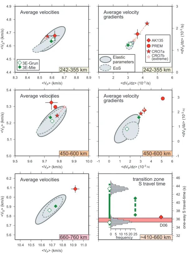
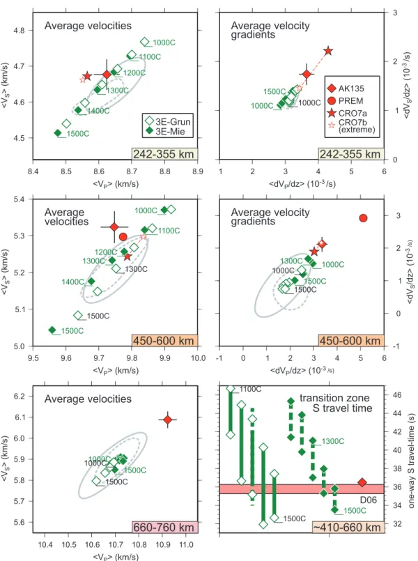
Figure 2. Effect of mineral physics uncertainties for 1300◦C adiabatic pyrolite on average velocities, average velocity gradients, and SS-precursor travel times, at a range of depth intervals. Adiabatic pyrolite models are green; seismic constraints are shown in red. D06 is globally averaged SS-precursor travel time through the transition zone with±0.5 s uncertainty (Deuss 2006, personal communication). Solid grey line represents 95 per cent confidence contour for mineral elastic+anelastic parameter uncertainties. Dashed grey contour shows estimation of the extent of equation of state (EoS) uncertainties—inferred from Fig. B(3). Dashed black line indicates uncertainty in waveform inversion data. Error on AK135 shown with black cross. Even taking these uncertainties into account 1300◦C adiabatic pyrolite provides a poor fit to average velocity gradients in the upper mantle and to average velocities immediately below 660 km. We have not shown PREM for the 242–355 km depth interval. PREM includes a large discontinuity at 220 km, now thought not to be a global feature, and as such it does not give a realistic representation of the average velocities or gradients in this depth range.
S travel times). These adjustments are consistent with the changes required to fit the average velocities and gradients.
A more quantitative, but less familiar, presentation of these results is shown in the lower half of Fig. 3. On the left-hand panel, we show
the mean travel time anomaly for the entire epicentral distance range studied. Our 13AP models tend to show negative anomalies on average (i.e. are too slow relative to observed travel times) in both P and S, but, given the magnitude of the elastic parameter and
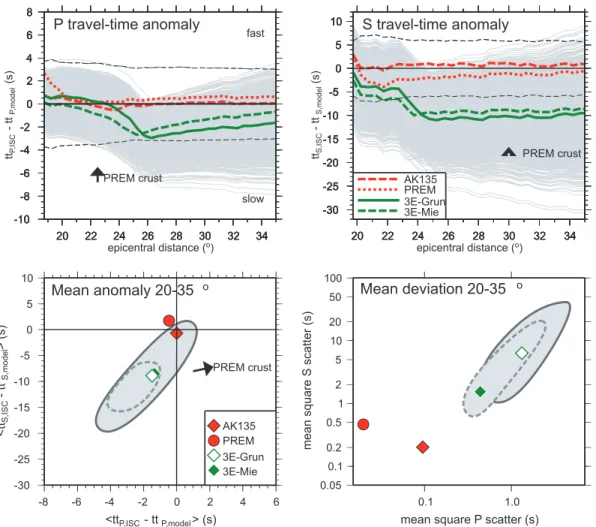
Figure 3. Effect of mineral physics uncertainties for 1300◦C adiabatic pyrolite on direct P and S arrival times. Arrival times are taken from reprocessed ISC catalogue (Engdahl 2000, personal communication). 1300◦C-adiabatic-pyrolite (13AP) models are green, with grey uncertainty distributions; seismic reference models are red. Black arrow shows shift in travel times due to changing crustal structure from AK135 to PREM. The upper panels show travel time misfit versus distance for P (left-hand panel) and S (right-hand panel) waves: anything which lies above 0 has shorter travel times than observations, i.e., is faster than the Earth, while anything below 0 has longer travel times than observations, i.e., are slower than the Earth. The lower right-hand panel shows the average value of the anomalies plotted in the upper panels, while the lower left-hand panel shows the amount of scatter of the travel time anomalies about their mean value. A large degree of scatter for all 13AP models, compared to AK135 and PREM, suggests significant structural complexity in the depth interval 450–900 km.
lithospheric structure uncertainty effects combined, may still be consistent with the ISC data. The right-hand panel shows the mean square scatter of the travel time anomalies about their mean value— a point plotting at (0, 0) would be a completely flat line in the travel time versus distance plots above. Clearly, even taking uncertainties into account, the misfit of our models is large compared with the seismic reference models PREM and AK135.
Summary
Figs 2 and 3 illustrate that mineral physics uncertainties translate into a large degree of seismic variability. Overall the variability due to uncertainties in the velocity calculation procedure is less than that due to mineral elasticity/anelasticity uncertainties. The effect of anelasticity is small, relative to that of elastic parameter uncertainties (Appendix B).
Nonetheless, certain seismic trends in our 13AP models—namely too low gradients in the depth intervals 242–355 km and 450– 600 km, and too low velocities between∼660–760 km—remain, even after taking the effects of all these uncertainties into account. This suggests that the average mantle physical structure may indeed
deviate from 1300◦C adiabatic pyrolite. To test this hypothesis, we begin by investigating alternative thermal structures.
(B) Alternative thermal structures
Under the premise of vigorous, whole-mantle convection, mantle temperature structure has traditionally been modelled as an adiabat, e.g. Brown & Shankland (1981) and Spiliopoulos (1984). However, recent evidence suggests that, in the lower mantle at least, a some-what sub-adiabatic profile may be more appropriate, to allow for a significant contribution from internal heating (Bunge et al. 2001; Monnereau & Yuen 2002). In addition, a different style of man-tle convection from the widely-used ‘whole-manman-tle’/‘single-layer’ model would lead to a non-adiabatic thermal structure.
For example, a thermal boundary layer could arise at the base of the upper mantle, if the viscosity increase associated with the phase transitions occurring around 660 km depth were sufficiently high to hamper convective flow across the boundary. Since the potential temperature at the base of the lithosphere has been constrained to within∼1350 ± 100◦C (McKenzie & Bickle 1988; Herzberg 1992; Green et al. 2001), we would expect a relatively hot lower mantle
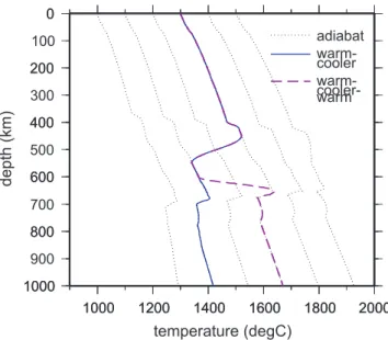
Figure 4. T –z profiles for adiabats with potential temperatures between 1000 and 1500◦C (dotted black lines). Solid blue and dashed purple lines are examples of alternative non-adiabatic structures tested against the seismic data.
with respect to the overlying upper mantle under these circum-stances. Alternatively, in the ‘plume-fed asthenosphere’ scenario envisioned by Morgan et al. (1995), in which hot material from up-welling plumes spreads out beneath the lithosphere, a temperature inversion structure would be generated, leading to a relatively cool transition zone and lower mantle.
However, the difference between adiabatic and non-adiabatic temperature gradients is small in the upper mantle, due to its relative thinness. Additionally, the relationship between temperature and seismic behaviour will be illustrated most effectively by retaining an adiabatic thermal structure, and shifting the potential tempera-ture (Tpot) to values hotter and colder than 1300◦C, while keeping all other physical parameters in our mantle models unchanged—rather than experimenting initially with possible non-adiabatic structures. We therefore begin by calculating the seismic properties along adi-abats whose potential temperatures range from 1000 to 1500◦C (Fig. 4, calculation detailed in Appendix A). Since the compari-son with the seismic data below illustrates that no single adiabatic structure reduces the misfit, then subsequently we consider whether some dynamically plausible non-adiabatic thermal structure may allow a pyrolitic mantle model to fit the seismic data.
(i) Different potential temperature (Tpot) adiabats
Average P- and S-velocities scale approximately linearly with po-tential temperature (Fig. 5). In the upper-mantle depth intervals, models which are slightly colder—i.e., faster—than 1300◦C adi-abatic pyrolite, by ∼100◦C, fit the inversion data as well as a 1300◦C adiabat, while adiabats warmer than Tpot ∼ 1350◦C can be ruled out because they are too slow. However, simply using a colder Tpot adiabat cannot reconcile our models with all seismic data, because changing temperature has little impact on the average velocity gradients. And in the lower mantle, none of the inves-tigated range of adiabats reconciles the models with the seismic average velocity constraints. This implies a more complex structure is needed.
This is further confirmed by the direct travel time misfits (Fig. 6), where colder adiabats improve the fit of the mean trav-eltime anomaly (most sensitive to average velocities), but not of the mean square scatter which reflects transition zone structure.
In contrast to the average velocities and average direct travel times, the SS-precursors are best fit by adiabats which are slightly warmer than 1300◦C, i.e., Tpot∼ 1400◦C, as opposed to colder. An increase in temperature results in a net transition-zone travel time decrease, because the traveltime is more heavily influenced by the resulting reduction in thickness of the transition zone, than by the associated decrease in velocity.
Thus, no single adiabat can fit all observations at all depth ranges, so either a more complex (non-adiabatic) thermal structure is needed, or an alternative chemical structure.
(ii) Alternative thermal (i.e. non-adiabatic) structures
Given the results of the previous section, we consider the possibility that there exists some non-adiabatic thermal structure which allows our pyrolitic mantle models to fit the seismic data. What would the form of such a model be? In Fig. 4, we have drawn some examples of the types of alternative thermal structure which we tested.
Both 242–355 km and 450–600 km require higher average ve-locity gradients than occur with adiabatic pyrolite. Section (Bi) il-lustrated that colder adiabats increase average velocities but do not affect velocity gradients. So, in order to increase velocities more rapidly with depth using thermal effects, a negative temperature gradient would be required. We experiment with this possibility for 450–600 km, because it is conceivable that accumulation of sink-ing slabs in this depth interval could be a plausible mechanism for generating a negative temperature gradient, on average. However, our results are applicable to any depth interval in which an increase in velocity gradients is required.
We used Fig. 3 to infer the approximate depth at which a tem-perature drop within 450–600 km should commence: we require P travel time anomalies to increase at the distance where, under an adiabat, they first begin to slope downwards (i.e.∼22◦). By trial-and-error we found that temperatures should start to fall at ∼450 km.
Fig. 7 shows the effect of different magnitude temperature drops, introduced smoothly over 450–550 km (as illustrated in Fig. 4, solid purple line), on seismic behaviour. Only average velocity gradients, transition-zone and direct travel times misfit structure are displayed: The effects on average velocities and mean travel time misfits are small (and consistent with the seismic data) for the thermal struc-tures being considered.
The average velocity gradients at 450–600 km increase fairly linearly as the magnitude of the temperature drop increases (top panel, Fig. 7), and having a temperature drop of∼200◦C provides an excellent fit to the seismic inversion data. Such a drop in temperature at 450–550 km also reduces the misfit to direct travel time data (but not by a large enough amount to be comparable with the seismic references AK135 and PREM) (bottom panel, Fig. 7).
Retaining lower temperatures until below the base of the transi-tion zone causes SS-precursor travel times to be too long (middle panel, Fig. 7), because the thickness of the transition zone increases at low temperatures. SS-precursor times will only match seismic data if a return from colder to warmer temperatures (at least to Tpot ∼ 1300◦C) takes place before the 660-phase transitions (Figs 4 and 7). However increasing temperatures above 660 km will
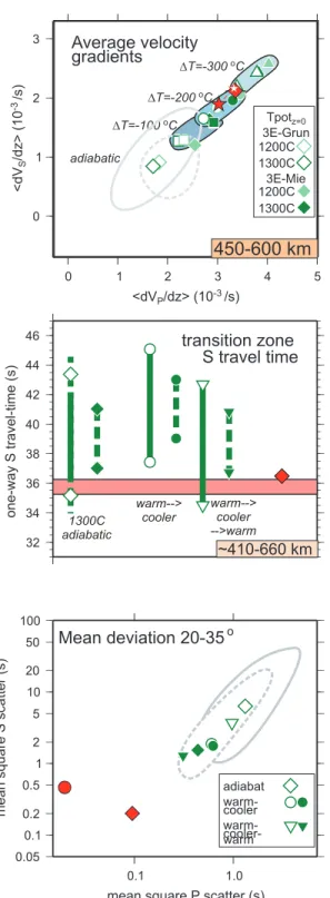
Figure 5. Seismic behaviour of different potential-temperature adiabatic pyrolites between 242 and 760 km. Refer to Fig. 2 for further explanation of symbols. Average velocities and travel times change approximately linearly with potential temperature, but velocity gradients are largely unaffected by constant temperature shifts and still do not fit the seismic data. Average velocities favour slightly cooler than 1300◦C models, whereas SS-precursors favour slightly warmer than 1300◦C models, for the transition zone.
increase the direct travel time misfits, which require high velocities below 660.
Thus, whilst having a cool lower transition zone is potentially geodynamically viable—for example, it could be consistent with a negative thermal anomaly from pooling slabs above the 660-discontinuity—the magnitude of its effect appears insufficient to fit all the seismic data simultaneously. Additionally, a thin, hot thermal
boundary layer between 600 and 660 km can not be fully ruled out. However, it would need to have also a low amplitude, not more than 50–100◦C, in order to fit SS-precursors and not worsen the misfit to direct P and S travel times. And this does not solve the misfit below 660 km depth.
It is presumably possible to generate a similar thermal structure which will fit the velocity gradients at 242–355 km, though we
Figure 6. Direct P- and S-travel time misfits for adiabatic pyrolites at a range of potential temperatures (1000–1500◦C). Refer to Figs 2 and 3 for further explanation of symbols. The mean square misfit (right-hand panel) is not reduced by uniform shifts in adiabatic temperature.
cannot conceive a physical mechanism for generating such a com-plex structure. Overall, we conclude that there may exist a thermal structure which provides an improved fit to all the seismic data than an adiabat, but our tests show that the magnitude of the improvement seems to be small, relative to the complexity of any such thermal structure, and the geodynamic plausibility of such a structure is questionable.
(C) Alternative chemical (i.e. non-pyrolitic) structures
Pyrolite is the most commonly accepted average composition for the upper mantle. However, significant chemical heterogeneity is to be expected here: Melting of a pyrolitic source rock to produce basaltic oceanic crust (MORB) leaves behind a harzburgitic residue. Dur-ing subduction, significant quantities of both the MORB crust and harzburgite-enriched subcrustal lithosphere are plunged back into the deeper mantle. Relative to pyrolite, MORB is strongly depleted in MgO, and enriched in SiO2, FeO, CaO and Al2O3,whilst harzbur-gite is correspondingly enriched in MgO and depleted in the other oxides (Table 1). These chemical differences give rise to distinct seismic behaviour in the three compositions (Fig. 8). Most striking are: the elevation of 410 and depression of 660-discontinuties in MORB, relative to pyrolite; slight depression of 410 and elevation of 660 in harzburgite; higher velocities in both MORB and harzbur-gite within the transition zone; and a significantly larger velocity jump at the 660-discontinuity in harzburgite. Thus, if there were sufficient pooling or enrichment of either of these components at any particular depth interval in the mantle, it could cause average seismic behaviour to deviate from that predicted for pyrolite.
We therefore calculate the seismic properties of both MORB and harzburgite (Fig. 9). Following Stixrude et al. (2006) we also test a mechanical mixture of 80 per cent harzburgite, 20 per cent MORB—the mixture whose bulk composition is approximately equal to pyrolite—in which we sum together the mineralogies cor-responding to harzburgite and MORB in the ratio 4:1, and compute the overall seismic velocities.
For all our non-pyrolite models, we input the same thermal struc-ture, the Tpot= 1300◦C adiabat of pyrolite. While altering compo-sition would cause the P–T path of an adiabat to change, keeping the temperature structure fixed allows us to understand the seismic effect of composition uniquely. Additionally, the magnitude of any change to the adiabats is relatively small.
Above the transition zone: 242–355 km
Given the elastic parameter uncertainties, harzburgite has aver-age velocities consistent with the seismic data, as does a MORB-harzburgite mechanical mixture which is enriched in MORB-harzburgite (Fig. 9). Our calculated average velocities for 100 per cent MORB, however, are much higher than the seismic inversion data.
MORB is the only chemical composition of the three end-members which has significantly different (high) average velocity gradients from the others (Fig. 9). This arises from the sharp velocity discontinuity around 280 km (Fig. 8) in MORB, which corresponds to the phase transformation of coesite to stishovite. As calculated according to our mineral physics database, 100 per cent MORB has too high gradients. However, a MORB-harzburgite mechanical mixtures plot on a mixing line between the 100 per cent MORB and 100 per cent harzburgite data points, and the mixture of 20 per cent MORB 80 per cent harzburgite has gradients almost identical to the inversion data. Such a mixture can thus reconcile average velocities as well as average gradients in this depth range.
The precise phase relations for MORB at this depth interval are uncertain—if the large velocity discontinuity at ∼280 km were actually smaller, the effect on average gradients would be corre-spondingly smaller. Nonetheless, according to a recent compila-tion, a discontinuity in this depth range is regularly observed (e.g. Williams & Revenaugh 2005). If the velocity jump were smaller than our calculations predict, then simply having a larger propor-tion of MORB in the mechanical mixture than 20 per cent would fit the data, and the discontinuity would not need to occur globally to be able to bias the global average sufficiently to increase average gradients.
Within the transition zone: 450–600 km
Noting that MORB and harzburgite are both faster than pyrolite in the transition zone, but have similar gradients to pyrolite (Fig. 8) we test models in which the composition is initially pyrolite but be-comes either MORB-and/or harzburgite-rich within the transition zone—since changing from 100 per cent pyrolite to a faster com-position will increase the gradients here, as required by the seismic data.
We find that models which become non-pyrolitic below 550 km have increased velocity gradients relative to pyrolite that are
Figure 7. Alternative, non-adiabatic thermal structures tested against seis-mic data. Introducing a drop in adiabat temperature of∼200◦C in the lower transition zone (irrespective of the absolute temperature) improves the fit to the velocity gradients, but a return to warmer temperatures is required to fit the SS-precursors, and does not significantly improve the fit to direct travel times. Refer to Figs 2 and 3 for further explanation of symbols.
consistent with the seismic data (Fig. 9). Average velocities are ac-ceptable for such all models. Once again, MORB–harzburgite me-chanical mixtures plot on a mixing line between 100 per cent MORB and 100 per cent harzburgite for both the average velocities and the average gradients, such that a mixture of 80 per cent harzburgite and 20 per cent MORB fits the data well.
Table 1. Bulk chemical compositions tested in this study.
Mol per cent SiO2 MgO Al2O3 FeO CaO
Pyrolitea 38.61 49.13 2.77 6.24 3.25
Harzburgiteb 36.22 57.42 0.48 5.44 0.44
MORBc 53.82 13.64 10.13 8.80 13.60
aSun (1982).
bIrifune & Ringwood (1987).
cPerrillat et al. (2006).
Models which are harzburgitic immediately above the 660-discontinuity fit SS-precursors well for 1300◦C adiabats (often bet-ter than the pyrolites fit), and no change in temperature is needed (Fig. 9). The improved fit relative to equivalent-temperature py-rolites is predominantly due to having a slightly shallower 660-discontinuity in harzburgite than pyrolite. (Models which are also harzburgitic above 550 km have the shortest times because of a deeper 410-discontinuity). MORB does not have a discontinuity until about 800km (Fig. 8) so although not plotted, MORB-based models will certainly be too slow.
Just below the transition zone: 660–760 km
The only chemical composition whose average velocities are com-parable with AK135 is harzburgite. Combining harzburgite with any other composition simply reduces its average velocities, making them less favourable. In fact, assuming our MORB phase diagram in this depth interval is reasonably accurate, we can positively rule out the possibility of a large (greater than∼20–30 per cent) MORB component in this depth interval, as MORB has such low velocities, owing to its much-delayed garnet to perovskite phase transitions. As discussed above, a harzburgitic composition below 660 is also compatible with SS-precursor transition-zone travel times.
Full depth range—direct traveltime fits
Direct P and S travel time anomalies represent the sound speed structure throughout the entire depth interval which the waves tra-verse. So for our range of epicentral distances, this is everything from approximately 0 to 900 km (but with the highest sensitivity to ∼430–900 km). For this reason, we have decided to illustrate what happens when all the compositional effects found to improve the seismic data as discussed above are implemented simultaneously.
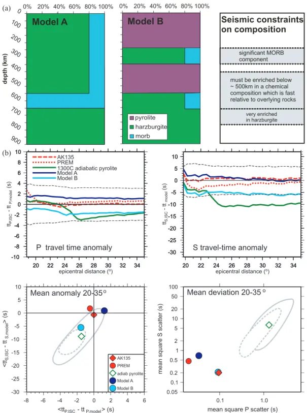
We show two plausible models (Fig. 10a). These models are by no means either unique or the best solutions to the seismic data—indeed they are extremely simple and structurally coarse, and better fits may be possible with more detailed structures. However, they satisfy the criteria identified, in the previous sections, as necessary for fitting the seismic data, i.e., a significant MORB component between ∼250 and 350 km; a shift to a seismically faster composition within the mid-lower transition zone; and extreme harzburgite enrichment immediately below the 660-discontinuity.
Both models demonstrate significantly better fit to direct travel times than adiabatic pyrolite (Fig. 10b). Although not plotted, the one-way S travel time (through the transition zone) for Model A is ∼33.4–37.4 s and for Model B is ∼35.2–40.4 s, so both models are also consistent with the SS-precursor data.
We stress that the models should not be interpreted as depicting a uniformly layered mantle, but rather one in which the global average structure is being biased by certain end-member three-dimensional structures which occur at different depth intervals.
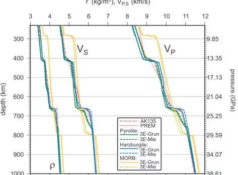
Figure 8. Density, VPand VS profiles for the three end-member compositions pyrolite, harzburgite and MORB (as defined in Table 1), and the seismic
references AK135 and PREM.
Additionally, the composition of the lower transition zone re-quired to fit the seismic data is entirely dependent on the com-position of the overlying mantle, and can be either MORB or harzburgite-rich (or both). If the upper transition zone is predomi-nantly pyrolitic, then either MORB or harzburgite-enrichment in the lower transition zone will increase the velocity gradients. However, if the upper transition zone is already predominantly harzburgitic, then the lower transition zone must be enriched in MORB relative to the overlying material in order to increase the gradients. However, the MORB component in the upper transition zone cannot be too large, or average velocities become too high.
D I S C U S S I O N
Further uncertainties
Seismic data reliability and coverage
We have identified a set of physical criteria required to fit the seismic data (see previous section). These criteria are sufficiently robust that they satisfy three independent seismic data sets (ISC direct travel times, surface wave inversions, and SS-precursor travel times) si-multaneously, and this should compensate for any systematic errors in the data sets. Additionally, all our data sets are extremely large, such that the effect of random errors is minimal, and most of the seismic variables we test against are extremely tightly constrained. The greatest source of uncertainty is the ISC database, as the distance we study overlaps with a triplication zone due to the 660-discontinuity (the triplication zone for 410 is outside the range of our data). This could lead to systematic mis-picking at epicentral distances of∼22◦, whereby the arrival that has propagated in the mantle below 660 is picked instead of the one which travelled above 660 (because the former arrives earlier). However, if this were the case in our data set, it would mean that the travel time anomalies of our models at around 22◦ should, in reality, be more positive than they currently plot (see Fig. 3). This in turn would increase
the size of the drop to more negative anomalies that happens for pyrolite models at mid-epicentral distances (∼23–25◦), increasing the misfit of pyrolite. So in fact, even if there were some bias in the direct travel times due to mispicking of arrivals, the effect of that bias would be that we have underestimated the misfit of pyrolite to the data.
The surface waveform inversions and SS-precursor travel times have global coverage and give a good representation of the 1-D average structure of the mantle. However at upper mantle depths the ISC travel time data and AK135 (which was created using travel time data) are both biased towards subcontinental/subduction zone mantle structure. Subcontinental and subduction zone mantle structures are not necessarily the same as suboceanic structure— we would expect the former to incorporate more slab material, for example. This can explain much of the discrepancy between AK135 and the surface waveform inversion data for average velocities and gradients—for example, higher gradients in AK135 at 450–600 km would be consistent with having a larger proportion of seismically fast slab material, and when comparing our models with AK135 we should be aware of the potential bias in AK135.
Mineral elastic parameter uncertainties—sampling and extrapolation
Thermochemical interpretation of our results is based on the premise that we have accurately gauged the magnitude of the error on our model velocities and travel times due to elastic parameter uncertainties. A key issue is whether our set of 10 000 random models fully samples the (elastic parameter) uncertainty solution space. Although this is not a large number of models given that we explore a 28-D parameter space, tests both we and Cammarano et al. (2005a,b) performed indicate that the range of seismic char-acteristics does not expand further when the number of models is increased (Appendix B).
As part of this study we have now done a more comprehensive analysis of the uncertainties in the equation of state than Cammarano
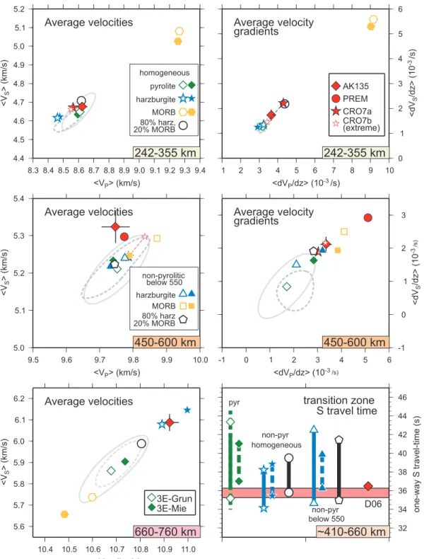
Figure 9. Average velocities, velocity gradients, and SS-precursor travel times for different chemical compositions at different depth intervals. Grey contours show model uncertainties as defined in Fig. 2. For 242–355 km and 660–760 km we show uniform non-depth varying compositions. Within the transition zone, that is, 450–600 km and SS-precursor models, we have plotted models which change from pyrolitic above 550 km to non-pyrolitic below 550 km. At all depth intervals, compositions which deviate from pyrolite significantly improve the fit to the seismic data.
et al. (2005a,b). Available experimental data cannot conclusively discriminate between different equations of state. Although we orig-inally found that the linear Gr¨uneisen thermal extrapolation (3E-Grun) best fitted the few published data sets of elastic parameters versus temperature, these results were all at low pressure and may not be appropriate if temperature dependence varies with pressure, as is implicit in the Mie-Gr¨uneisen thermal correction (3E-Mie).
This issue could be further explored if more data becomes avail-able either through more high pressure experiments or ab initio calculations.
However, with our best estimates of both types (i.e. elastic pa-rameters and EoS) of uncertainty, our results show that even when adding the two effects, adiabatic pyrolite misfits seismic constraints in several respects, most notably the gradients between 242 and
(a)
(b)
Figure 10. (a) Two seismically plausible alternative average composition–depth profiles for the upper mantle. Panel on the right-hand side indicates seismic constraints inferred at different intervals. (b) Fit to direct P and S travel times of suggested alternative compositions illustrated in (a). The degree of misfit for these two models is very small and comparable in magnitude to the seismic references AK135 and PREM.
350 km and the average velocities below 660 km. The discrepancy with gradients between 450 and 600 km is slightly more tentative, as the 3E-Mie model data point, with a different equation of state as well as different data, almost satisfies seismic constraints here (Fig. 2). However from our analyses, the 2005 database used for this point is an end-member case within the transition-zone lit-erature data and the more recent 2007 database again leads to a significant mismatch (Appendix B). Ultimately, we cannot rule out
the possibility that adiabatic pyrolite may fit the velocity gradients for this depth interval, but the compositional changes we have sug-gested for this depth interval not only appear to be more compatible with the seismic data—simultaneously fitting direct and transition-zone travel times and velocity gradients (adiabatic pyrolite does not fit direct traveltimes even with 3E-Mie), but they are also in line with our observation that chemical changes are required in the other depth intervals. Additionally, other workers have found, with
a recently obtained data set, a need to change the composition in this depth interval (e.g. Irifune et al. 2008).
Phase equilibria
Dynamic interpretation of our improved-fit physical models is based on the assumption that the mineral phase relations we used for py-rolite, MORB and harzburgite are reasonably accurate. Most un-certain are sublithospheric phase relations in MORB—crucially whether our ‘280’ and ‘790’ km discontinuities (Fig. 8), and very high upper-mantle velocities, are correct—because current experi-mental data for the constituent minerals of MORB at high pressures are extremely limited. In addition, the 5-oxide system we use in our calculations provides a good representation of pyrolite and more depleted (harzburgitic) compositions, but is less appropriate for MORB where other oxides, for example, Na2O and K2O, make up a greater proportion of the composition. However, the key features of our MORB phase diagram are in good agreement with both the recent experimentally determined phase diagram of Perrillat et al. (2006), and another thermodynamically derived phase diagram by Ricard et al. (2005). Each of these diagrams places the garnet to perovskite transition at depths greater than 700 km—i.e., well below the 660-discontinuity of pyrolite—and we feel this is therefore a ro-bust feature of our results. Less certain is the depth of the coesite to stishovite transition, which is placed below 350 km by Ricard et al. (2005). Nonetheless, having the transition take place between 250 and 350 km provides a simple solution to the seismic characteristics of this depth interval, and others (e.g. Williams & Revenaugh 2005) have proposed that the transition should lie within this depth range. Asides from the coesite to stishovite discrepancy, our density and velocity profiles for pyrolite, harzburgite and MORB (Fig. 8) are similar to those of Ricard et al. (2005), which lends support to our findings.
Figure 11. Themochemical model of Tackley et al. (2005). It has a smooth, monotonically increasing temperature profile, and has changes in composition with depth consistent with our results.
Implications for average physical mantle structure
Mantle dynamics
Our results strongly suggest that significant deviation from pyrolite, as well as vertical chemical variability, is necessary to fit seismic data for the upper mantle and transition zone. This is consistent with the most recent geodynamic models by Tackley et al. (2005), in which average mantle composition is continuously changing with depth, and rarely 100 per cent pyrolitic (Fig. 11). The key features of Tackley et al. (2005)’s profiles are compatible with our best-fitting models. Most notably their models incorporate enrichment in MORB in the lower part of the transition zone, followed by a shift to harzburgite-rich composition at and below the 660-discontinuity, similar to our Model A (Fig. 10a). The density profiles in Fig. 8 il-lustrate why this compositional segregation occurs: in this interval, behaviour is dominated by the different depths at which the phases present transform to perovskite. In simple terms, olivine-rich ma-terials transform to perovskite at shallower depths than garnet-rich ones, for temperatures close to the 1300◦C adiabat. Al-rich garnet is more dense than olivine, and once garnet has transformed to perovskite, that perovskite is more dense than Al-poor perovskite. However, garnet is less dense than both Al-rich and Al-poor per-ovskite. So in MORB, a lack of olivine-component and enrichment of garnet-component means that the bulk transition to perovskite is delayed by∼100 km depth relative to pyrolite and harzburgite, making the MORB buoyant over the depth interval∼650–800 km. Harzburgite meanwhile, depleted in the garnet-component, attains a higher density than pyrolite until about 750 km at which point suf-ficient excess garnet in the pyrolite has transformed to perovskite to give pyrolite a higher density than harzburgite. So different compo-nents accumulate at depths at which they become neutrally buoyant. Numerical modelling (Tackley et al. 2005; Mambole & Fleitout 2002) indicates that the mechanism for this segregation is not
delamination of slabs as they pass through the transition zone— where high viscosity hampers separation—but rather that they sep-arate in the deeper mantle after having warmed and softened, and then accumulate at different depths as they rise. The average chem-ical gradients do not imply that the mantle is convectively layered, but rather represent an average of significant lateral chemical het-erogeneity, which has a tendency to pool more or less in specific depth ranges within a whole mantle flow pattern.
Our seismic data do not distinguish between sharp discontinu-ities or gradational changes. So, while we have assumed discrete compositional layering in our models, and have increased the ve-locity gradients in both the upper mantle and the transition zone by introducing sharp discontinuities for these depth intervals, more gradational changes showing the same trends should also fit. How-ever, we speculate that a sharp structural boundary due to local heterogeneity around 500–550 km could actually be responsible for the regularly observed (e.g. Shearer 1991; Flanagan & Shearer 1998; Deuss & Woodhouse 2001) 520 km seismic discontinuity, and would be consistent with our results. This is as opposed to the traditional view of the 520-discontinuity being caused by the phase change from wadsleyite to ringwoodite (e.g. Sawamoto et al. 1984; Weidner et al. 1984; Shearer 1990), since very few of our 10 000 adiabatic pyrolite models have a positive velocity discontinuity at this depth (Fig. 1), and even when they do, it is not sharp enough to match seismic observations. An earlier study by Rigden et al. (1991) also indicated that the 520-discontinuity may not arise from the wadsleyite to ringwoodite phase transition.
Alternative solutions
We have demonstrated that it is possible to reconcile our mantle models with seismic data using only changes in bulk chemical com-position with depth, and that thermal structure need not deviate from adiabatic necessarily. It is also possible to reduce the seismic data misfit thermally—albeit with a lot of structural complexity to give relatively minor improvements—but it is not possible to completely alleviate the misfit with seismic data purely thermally. We cannot exclude the possibility of chemical variations together with some small (<50–100◦C) variations around an adiabatic temperature pro-file. However, the dynamic models of (Tackley et al. 2005) display smooth, monotonically increasing average temperature profiles (see Fig. 11).
Changing the bulk composition and/or temperature are not the only means of fitting the seismic data. A different anelasticity struc-ture could reduce the misfit of adiabatic pyrolite to the data: in-creasing Q in the transition zone increases average velocities and velocity gradients, thereby producing a better fit to travel time data. However we find that very extreme Q values (Qs greater than∼700) are needed to fit the data, and this is incompatible with observed values of seismic attenuation (Cammarano & Romanowicz 2008).
Alternatively, minor constituents which we did not model in our simulations, most notably water, could influence seismic properties appreciably. Wadsleyite and ringwoodite, the major silicate minerals of the transition zone, have much higher water solubilities than both the olivine which overlies them (Young et al. 1993; Kohlstedt et al. 1996), and the perovskite underlying them (Bolfan-Casanova et al. 2000; Bolfan-Casanova et al. 2003), so it has been suggested that the transition zone could potentially host significant amounts of water (Bercovici & Karato 2003).
To estimate the potential effect of water, we ran tests in which we adjusted the bulk modulus; shear modulus; their pressure
deriva-tives, and the density, of wadsleyite and ringwoodite, to values re-ported for their hydrated counterparts (see Cammarano et al. (2003) for these values, and the references from which they were obtained), assuming a water content of 2 per cent. This percentage probably represents an upper limit on the water content of the transition zone: the maximum hydration of wadsleyite seen during experiments has been about 3 wt% H2O (Inoue et al. 1995), but when the presence of water in the transition zone has been inferred from observations, both seismically (e.g. Van Der Meijde et al. 2003) and from electri-cal conductivity (Huang et al. 2005), values have typielectri-cally been an order of magnitude lower than this.
Hydrating wadsleyite and ringwoodite by 2 per cent reduces both their seismic velocities—so potentially, hydrating the wadsleyite but not the ringwoodite could be used as a means of increasing the velocity gradients within the transition zone. However, the degree of hydration required to create this effect (2 per cent) is large, and it is difficult to envisage a mechanism by which wadsleyite is hy-drated but ringwoodite is not. If both minerals are hyhy-drated, then the velocity gradients actually decrease. Additionally, making the wadsleyite zone slower makes the direct travel time anomalies more negative, and we have seen that 1300◦C adiabatic pyrolite already tends towards being too slow in this depth interval (Figs 2 and 3). Hence, our tests suggest hydration cannot solve the discrepancy be-tween pyrolite and the seismic data. However, without more mineral physics data for hydrous phase equilibria, or for minerals contain-ing trace elements (such as Na), we cannot completely exclude the possibility that this or some other minor element could influence the problem—although we would expect such effects to be minor due to their minor abundance.
Concluding remarks
We have created a set of 1-D physical models which, taking ther-modynamic uncertainties into account, provide a more acceptable fit to global average seismic data sets than adiabatic pyrolite. How-ever these models are unlikely to represent a ubiquitous average mantle structure. More likely, the global average seismic properties which we observe for the mantle are being biased by certain regional structural features—such as subducting slabs—which dominate the mean seismic signal by ‘pulling’ it in a particular direction away from what we might expect the background structure (adiabatic pyrolite?) to be.
This in turn implies that the 1-D reference velocity models such as PREM and AK135 do not correspond to a specific physical struc-ture, and instead are variably influenced by different components of a three-dimensional mantle. If this is indeed the case, then we should no longer interpret tomographic images in terms of veloci-ties relative to these reference models. Instead, for a more accurate and quantitative analysis, we should move towards creating maps of absolute seismic velocity.
Finally, a more detailed and precise understanding of the structure and composition of the deeper mantle than that obtained here can only be achieved by reducing the uncertainties in the mineral physics computations. Such computations require more constraints on the values of elastic moduli for individual minerals, over the full range of mantle pressures and temperatures, as opposed to constraints on the behaviour of mineral aggregates taken to represent bulk mantle composition. In particular, clarification of the behaviour of mineral end-members found in extreme compositions such as MORB would be invaluable.